Development of a computational approach for the identification and annotation of transport proteins

Daniel Torres Varzim Faria

Development of a computational approach

for the identification and annotation of

transport proteins

Daniel Torres Varzim Faria

Development of a computational approach

for the identification and annotation of

transport proteins

Dissertação de Mestrado

Mestrado em Bioinformática

Trabalho efetuado sob a orientação de

Professor Doutor Oscar Dias

A

CKNOWLEDGEMENTS

/A

GRADECIMENTOS

Apesar deste trabalho ter sido realizado por mim tal não seria possível sem um grande grupo de pessoas que me apoiou durante todo o ano. Por esse motivo guardo a primeira seção do meu trabalho para agradecer o apoio de todas elas e quero realçar que sem elas não teria conseguido chegar tão longe.

Gostaria de agradecer aos meus orientadores, professor Oscar Dias e professor Miguel Rocha por todo o tempo dispensado para me ajudar e rever o meu trabalho, pelos seus conselhos e pela orientação nas horas em que me sentia mais perdido.

Aos colegas do grupo de investigação de Biossistemas por toda a simpatia e boa disposição demostrados no local de trabalho, principalmente ao Vítor Vieira, Fábio Ramalho e Filipe Liu por me terem ajudado nos momentos de maior dificuldade.

Um grande obrigado a todos os meus colegas de mestrado, pelo companheirismo, amizade e por todos os momentos de diversão que me proporcionaram ao longo do mestrado que vou guardar para sempre na memória. Queria agradecer também a todos os meus restantes amigos que, apesar de não me terem acompanhado neste percurso, estiveram sempre lá para me apoiar com palavras de apoio e força.

Um agradecimento para toda a minha família especialmente para os meus pais e irmão, por todo o carinho, força e conselhos que me deram ao longo da vida. Queria agradecer principalmente à minha mãe por ser um dos pilares da minha vida e por se ter sacrificado e trabalhado tanto para que eu pudesse estudar e fazer o que realmente gosto.

Quero agradecer também à minha namorada pelo apoio incondicional, pelo carinho, por nunca me deixar sentir em baixo e por sempre me incentivar a lutar pelos meus objetivos. Obrigado por seres um exemplo de perseverança, força e coragem para mim.

R

ESUMO

Na última década, dada a evolução nas técnicas de sequenciação de nova geração, o número de genomas sequenciados tem vindo a crescer exponencialmente [1]. A ferramenta merlin, desenvolvida pelo grupo de investigação Biosystems (Universidade do Minho) é uma ferramenta capaz de gerar modelos metabólicos à escala genómica. A identificação de genes que codificam proteínas transportadoras e os metabolitos transportados por estas são tarefas essenciais para o desenvolvimento de modelos metabólicos à escala genómica mais robustos e precisos.

Para este trabalho foram treinados e testados sete modelos de aprendizagem máquina diferentes, usando um processo validação cruzada repetido 5 vezes, em conjuntos de dados diferentes, para identificar e classificar proteínas transportadoras. Para provar o valor dos modelos desenvolvidos foram criados quatro conjuntos de dados diferentes compostos por proteínas curadas provenientes das bases de dados TCDB e SwissProt.

Os conjuntos de modelos criados usando vários conjuntos de dados apresentaram um bom desempenho global, com o melhor a atingir 91% de acerto e desvio padrão baixo; o valor de F1-score atinge os 0.90 (+/- 0.00), fazendo destes modelos uma boa solução para a identificação e caracterização de proteínas transportadoras dado um genoma não anotado.

Os modelos usados para identificar proteínas transportadoras apresentaram um maior número de falsos negativos comparado com o número de falsos positivos (quase três vezes maior) o que significa que os níveis de confiança para uma classificação em proteína transportadora são elevados, e que os modelos falham um número ainda significativo de proteínas transportadoras que são incorretamente ignoradas.

A

BSTRACT

In the last decade, given the evolution of next-generation sequencing techniques, the number of sequenced genomes has grown exponentially [2]. The framework merlin [1], developed by the Biosystems research group (University of Minho) is a tool capable of generating genome-scale metabolic models. The identification of genes encoding transport proteins and the metabolites transported by them are essential tasks for the development of more robust and accurate genome-scale metabolic models.

For this work, seven different machine learning models were trained and tested, using a five-fold cross validation process, on different datasets to identify and classify transport proteins. To prove the value of the developed models, four different datasets composed by well annotated proteins from TCDB and SwissProt were used.

Ensembles of the models created using different datasets showed good overall performance with accuracy reaching 91% and low standard error; F1 scores reach 0.90 (+/- 0.00), making them a good solution for the identification and characterization of transport proteins given a new unannotated genome.

The models used to identify transport proteins had a bigger number of false negatives compared to false positives (almost three times bigger) meaning that the confidence level of the classification of a protein as a transporter is high, and that these models miss a relevant number of transporter proteins that misclassified.

I

Acknowledgements/Agradecimentos ... iii

Resumo ... v

Abstract ... vii

List of Figures ... xi

List of Tables ... xiii

List of Abbreviations and Acronyms ... xv

1. Introduction ... 1

1.1 Motivation ... 1

1.2 Objectives ... 2

1.3 Structure of the document... 2

2. State of the art ... 5

2.1 Machine Learning concepts and definitions ... 5

2.2 Sequence analysis algorithms and tools ... 17

2.3 Relevant bioinformatics tools and databases ... 20

2.4 Relevant development environments ... 25

3. Methods ... 27

3.1 Data ... 27

3.2 Input attributes and output attributes ... 27

3.3 Data sets ... 30 3.4 Dataset pre-processing ... 31 3.5 Feature selection ... 32 3.6 Models ... 32 3.7 Ensemble Methods ... 33 3.8 Cross-validation ... 34 3.9 Performance evaluation ... 34 4. Development ... 35 4.1 Code Developed ... 35 4.2 Workflow ... 45

5. Results and Discussion ... 47

5.1.1 Case study: Transport and Transport related protein models performance ... 47

5.1.2 Case study: Influence of negative cases in model performance ... 54

5.1.3 Case study: Transport protein models performance ... 55

5.1.4 Case study: Transport proteins characterization models performance ... 56

6. Conclusions and further work ... 65

Bibliography ... 68

Attachment I ... 72

L

IST OF

F

IGURES

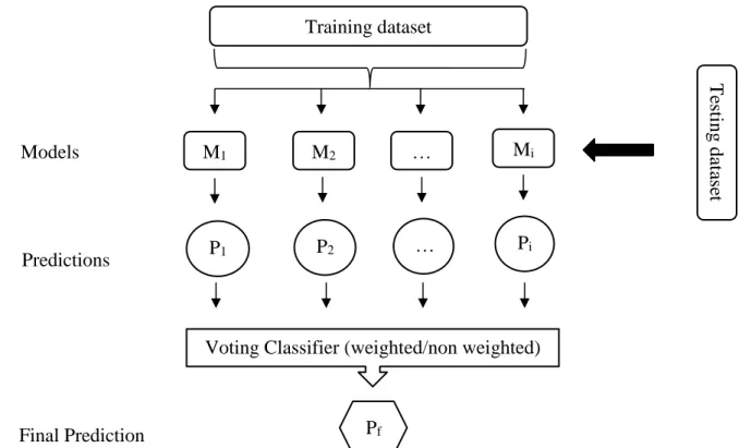
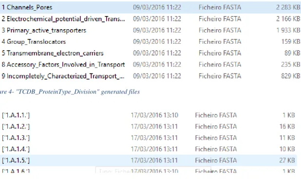
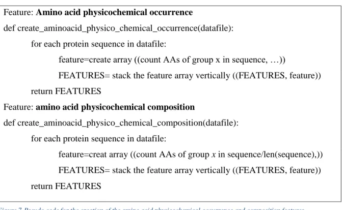
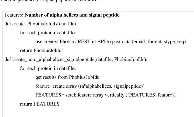
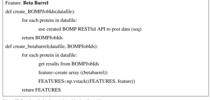
Figure 1- Seven step process for developing a machine learning algorithm ... 7 Figure 2-Calculation of the probability of classifying as “Yes” or “No” in the example “X1, Y2” ... 8 Figure 3- Voting classifier prediction method (Hard Vote classifier´s final prediction is the class predicted by most of the models, while weighted voting classifiers considers that each model has a weight given by the user. When making the final prediction, models with bigger weight have more influence in the final result. ... 33 Figure 4- "TCDB_ProteinType_Division" generated files ... 35 Figure 5- "TCDB_ProteinType_Division2" example of the generated files ... 35 Figure 6- Pseudo code for the creation of the amino acid occurrence and composition features ... 37 Figure 7-Pseudo code for the creation of the amino acid physicochemical occurrence and composition features ... 38 Figure 8- Pseudo code for the creation of the dipeptide composition feature ... 38 Figure 9-Pseudo code for the creation of the number of transporter related pfam domains feature ... 39 Figure 10- Pseudo code for the creation of the single transporter related Pfam domains feature ... 40 Figure 11-Pseudo code for the creation of the number of alpha helices and signal peptide features ... 40 Figure 12-Pseudo code for the creation of the beta barrel feature ... 41 Figure 13- Pseudo code for the location prediction feature ... 41 Figure 14-Pseudo code for the creation of the out attributes “Is Transporter” and “TCDB_ID” ... 42 Figure 15-Pseudo code used for mixing the final dataset and splitting it´s in and out attributes ... 43 Figure 16-Pseudo code for the data transformation, feature selection and model training and testing ... 44 Figure 17-Pseudo code for the ensemble methods “VoteClassifier” with hard voting and weighted hard voting ... 44

Figure 18-Pseudo code for the prediction method. Predicts if a protein is a transporter protein and if it is, predicts the first level of the TC system from 1 to 5. ... 45 Figure 19- Workflow of the developed algorithm ... 45

L

IST OF

T

ABLES

Table 1-Table containing the number of times a class occurs given a certain feature ... 8

Table 2-Confusion matrix example ... 13

Table 3-Different Models used by some Localization prediction tools and their respective websites. ... 21

Table 4- Overview of the objective and models used in some Membrane protein topology tools and their respective websites. ... 23

Table 5- Dataset1 content ... 31

Table 6- Dataset2 content ... 31

Table 7- Dataset3 content ... 31

Table 8- Dataset4 content ... 31

Table 9- Mean of PECC, F1 and ROC-AUC scores after a 5-fold cross validation process using Dataset1 without filters. ... 48

Table 10- Mean of PECC, F1 and ROC-AUC scores after a 5-fold cross validation process using a variant of Dataset1 with variance threshold filter. ... 49

Table 11- Mean of PECC, F1 and ROC-AUC scores after a 5-fold cross validation process using a variant of Dataset1 with StandardScaler(). ... 49

Table 12- Mean of PECC, F1 and ROC-AUC scores after a 5-fold cross validation process using a variant of Dataset1 with MaxAbsScaler(). ... 50

Table 13- Mean of PECC, F1 and ROC-AUC scores after a 5-fold cross validation process using a variant of Dataset1 with a Variance threshold followed by a RFE filter. ... 51

Table 14- Mean of PECC, F1 and ROC-AUC scores after a 5-fold cross validation process using a variant of Dataset1 with the best pre-processing parameters. ... 51

Table 15- Mean performance of the ensemble methods: “VotingClassifier” with and without weights on the models using a variant of Dataset1. ... 52

Table 16-Confusion Matrix for all models after a cross-validation process with training dataset representing 80% of the dataset1 and the test dataset the other 20%. ... 53

Table 17- Mean of PECC, F1 and ROC-AUC scores after a 5-fold cross validation process using a variant of Dataset2. ... 55

Table 18- Mean of PECC, F1 and ROC-AUC scores after a 5-fold cross validation process using a variant of dataset12345. ... 55 Table 19- Mean performance of the ensemble methods: “VotingClassifier” with and without weights on the models. ... 56 Table 20-- Mean of PECC scores after a 5-fold cross validation process using a variation of the transporter dataset. ... 57 Table 21-- Mean performance of the ensemble methods: “VotingClassifier” with and without weights on the models. ... 57 Table 22- Confusion Matrix for the NB model after a cross-validation process with training dataset representing 80% of the transporter dataset and the test dataset the other 20%. ... 58 Table 23- Confusion Matrix for the ET model after a cross-validation process with training dataset representing 80% of the transporter dataset and the test dataset the other 20%. ... 58 Table 24- Confusion Matrix for the KNN model after a cross-validation process with training dataset representing 80% of the transporter dataset and the test dataset the other 20%. ... 59 Table 25- Confusion Matrix for the LR model after a cross-validation process with training dataset representing 80% of the transporter dataset and the test dataset the other 20%. ... 59 Table 26- Confusion Matrix for the GB model after a cross-validation process with training dataset representing 80% of the transporter dataset and the test dataset the other 20%. ... 60 Table 27-Confusion Matrix for the RF model after a cross-validation process with training dataset representing 80% of the transporter dataset and the test dataset the other 20%. ... 60 Table 28- Confusion Matrix for the SVM model after a cross-validation process with training dataset representing 80% of the transporter dataset and the test dataset the other 20%. ... 61 Table 29-Table of sensibility and Specificity for each class predicted by every model ... 62

L

IST OF

A

BBREVIATIONS AND

A

CRONYMS

AA- Amino acid

ET- ExtraTreeClassifier GB- GradientBoostingClassifier KNN- K -nearest neighbours LR- Logistic Regression ML- Machine Learning NB- Naive Bayes RF- RandomForest

1. I

NTRODUCTION

1.1 Motivation

Genome-scale metabolic models are mathematical representations of living organisms. These models are sets of reactions and constraints, which mimic the behaviour of the organisms when exposed to different environmental and genetic conditions [1]. The identification of genes encoding transport proteins and the metabolites they carry are important tasks for the development of more robust and accurate genome-scale metabolic models [3].

Transporter proteins are polypeptide chains, which promote the transport of several compounds across cell membranes [4]. For instance, carrier proteins control the uptake of nutrients to the cell, thus being important for growth, and provide resistance to drugs, which allow organisms to thrive in severe conditions. These transporters may use several mechanisms to move the compounds, including facilitated diffusion, symport and antiport.

Manually annotated transporter proteins are described and stored in databases, such as the Transporter Classification Database (TCDB) [5]. TCDB is a curated repository for factual information compiled from literature references. It is available in a web-accessible relational database encompassing sequence, classification, structural, functional and evolutionary information for transport proteins from a variety of living organisms.

These proteins have several specific characteristics. For instance, they are usually found in membranes, they contain specific motifs on their tail residues [4], and usually have one or more transmembrane domains (alpha helices or beta barrels) on their sequences.

Transport proteins are usually annotated with reactions for metabolites known to be taken in from the medium, excreted from the cell or transported across intracellular compartments [6]. However, transport proteins are often poorly annotated [7] as this information is usually only retrieved from literature evidences.

In genome-scale metabolic models, transport reactions are usually added manually based on experimental data or literature. Thus, new methods that can automate this task are required [8]. Recently, the Biosystems research group (University of Minho) has published a framework, merlin [1], fully written in Java and that uses a MySQL database, which includes a tool that provides a first approach for tackling this problem. The Transport Reactions Annotation and Generation (TRIAGE) [9] tool identifies the metabolites transported by each transmembrane

protein and its transporter family. The localization of the carriers is also predicted and, consequently, their action is confined to a given membrane. This thesis proposes a different approach to this problem through the development and implementation of several machine learning models that can be used to identify and characterize transport proteins.

1.2 Objectives

The main goal of this work is the development of a machine learning framework which is able to identify and annotate transporter proteins from their amino acid sequence.

In detail, the technological objectives are:

1) To review relevant bibliography about the state of the art techniques and existing tools for the annotation of proteins, in general, and, more specifically, transporters; assessment of the main features that characterize transporter proteins;

2) Studying and testing available relevant software tools;

3) To develop a machine learning tool to annotate transporter proteins, involving: a) Selection of available tools that can be helpful for transporter annotation;

b) Development of machine learning methods for identifying transporter proteins, by developing classifiers and applying them to new sequences;

c) Development of classifiers to identify proteins able to transport specific metabolites; 4) Validation of the tool with gold standard corpora from previously manually annotated

sources and if possible in real world scenarios.

1.3 Structure of the document

This document is organized in the following way:

Chapter2 State of the art

Introduction to some machine learning concepts and models as well as some ensemble and feature selection methods and model evaluation processes. Brief presentation of useful bioinformatics tools and databases for the characterization of proteins.

Chapter3 Methods

Overview of the data collected to create the datasets. Description of the used dataset pre-processing, feature selection, models, ensemble methods and statistics to evaluate the models.

Chapter 4 Development

Brief description of the code developed in the thesis with pseudo code of the main scripts.

Chapter 5

Results and Discussion

Presentation of the main results generated in the thesis followed by a discussion of the results.

Chapter 6

Conclusion and Future Work

Main conclusion of the thesis taken from the results obtained, followed by a description of the possible improvements and future work.

2. S

TATE OF THE ART

2.1 Machine Learning concepts and definitions

One of the differences between a computer and a human being is that, when facing a problem, humans tend to try to improve the way they solve it, while computers only execute procedures supplied to them. Although computers may be very effective in solving problems they lack the ability of self-improvement with experience [10]. Machine Learning (ML) is a branch of artificial intelligence/ computer science/ statistics that provides computers with the ability of predicting the outcome of an event or situation, and eventually improving its results with time, simulating the gain of experience [11].

Tom Mitchell defines ML as “A computer program is said to learn from experience E with respect to some class of tasks T and performance measure P, if its performance at tasks in T, as measured by P, improves with experience E” [12].

In order to help the reader to understand the concept of ML, the next paragraphs contain a summary of some ML concepts and definitions [11][13][14].

Attribute. An attribute represents a feature that describes instances. Attributes can be

categorical or continuous. Categorical attributes take values from a set with a finite number of discrete values and can either be nominal, indicating that there is no order between the values e.g. names and colours, or ordinal e.g. little, medium, big, where an order can be identified. Continuous attributes take values from a domain which is a subset of real numbers and can take any value within a range e.g. height, time [14].

 Attribute values. For example, if “names” is an attribute, “John” is a value of the attribute “names”.

 Input and output attributes. Input attributes are the attributes that are going to be used to make a prediction of the output attribute.

Instance. Instance (or example) is an object composed by a set of input attributes (and possibly

the respective output attribute). Instances represent individual cases of the concept to be learned.

Dataset. A matrix of data, where each column represents an attribute, and each row represents

a different instance. Generally, the last column represents the output attribute, and the remaining represent the input attributes.

 Training Dataset. Group of instances that are used to learn the best model for that specific data.

 Test Dataset. Group of instances that are used to calculate different statistics on the generated model.

Model. A model can be defined as a function that given an instance´s input attributes predicts

its output attribute.

Algorithm. An algorithm defines a process that, given a training data set and some pre-chosen

criteria, chooses a specific model.

Supervised learning is a method that uses a given input data (training data set) to generate a model function that infers the underlying relationship between that data. Using that model, the result of the class label (out-attribute) can be predicted. This method is really useful when it comes to predict the class label of a data set with hidden phenomena attached in unfamiliar or unobserved data instances [11]. The errors associated with the prediction can be minimized based on the quality of the data set (training data set) used. Small data sets (20-30 examples) are generally a poor choice for these algorithms. Data sets that contain many similar examples can be a bad choice as well, since they can cause overfitting of the model. The best choice for a data set would be a data set that is a good representation of all possible instances (generalized) in order for the model to have an example of each possible outcome [11].

Development of ML algorithms. When developing a ML algorithm, 7 major steps should be

considered (Figure 1). The first one is to collect the data, where a subset of all available data attributes that might help in resolving the problem are selected. The second step is to process the data, making it understandable. Then the data is transformed, by feature scaling, decomposition, or aggregation (combining multiple instances into a single feature). The next step is to train the algorithm, where the training and testing datasets from the data previously transformed is selected. The algorithm is then trained (fourth step) using the training dataset, extracting the knowledge or information on that dataset, yielding a model that is a representation of that information. This model can then be used to predict the output attribute of other similar data.

Step five is where the algorithm using the test dataset is evaluated. In this step, evaluation of the effectiveness and performance of the model is performed. Giving the input attributes of the test dataset to the model, and hiding the output attribute, it predicts the output attribute for each instance. Comparing the two results, the known and the predicted, calculating different statistics about the performance of the model can be achieved. In the next step, the model created can eventually improve by using a different dataset or improving the old one. The last step is to apply the validated model, making reliable predictions on new datasets with unknown out-attributes.

Machine learning models and algorithms. The next chapter will review some of the major

models and algorithms used in ML, namely k-nearest neighbours (KNN), Naïve Bayes (NB), linear and logistic regression, decision trees, artificial neural networks (ANN), and SVMs (Support vector machines).

K-nearest neighbours (KNNs)

KNNs is an instance based learning method, meaning that it does not generate a model function. Instead, it stores the training set and uses it when a new prediction needs to be made, being called a lazy learning method for that reason, since it delays the learning process [13]. KNN has two simple ways of making predictions depending on the type of problem (classification or regression). In a classification problem, the algorithm will simply find the k training examples most similar to the new example to be predicted and the final prediction will be the most

Collect the data

Process the data

Transform the data

Train the algorithm

Test the algorithm

Improve the model created

Apply the model

common class on those k training examples. In a regression problem, the algorithm will predict the final result as the mean of the nearest neighbour values.

To calculate the nearest neighbours, a distance function must be used. For continuous (e.g. height) or linear discrete (e.g. number of children) features, Euclidean distance or Manhattan distance are usually used. For linear symbolic features (e.g. symptoms) the most common way of calculating their distances is to assume the value 1 for a different feature and the value 0 for an equal feature, and then calculate the examples distances using the Euclidean or Manhattan distance [13]. However, the previous method does not consider that some linear symbolic features may have an order, so a different distance function must be used. Value difference metric (VDM) considers two features to be closer if they have more similar classifications, thus ranking the features and providing a better calculation of the neighbours [15].

Naïve Bayes (NB)

NB is a simple algorithm that uses relative frequencies to estimate the probability of an example to present a certain result [13][16], assuming (although naively) the attributes are independent and cannot be differentiated in terms of importance. To better understand this algorithm, the data in Table 1 will be used.

Table 1-Table containing the number of times a class occurs given a certain feature

Attribute X Attribute Y

Class-Yes Class-No Class-Yes Class-No

X1 0 3 Y1 1 3 X2 5 1 Y2 4 1 Example “X1,Y2” 𝐿(𝑌𝑒𝑠) =0 5∗ 4 5∗ 5 9= 0 𝐿(𝑁𝑜) =3 4∗ 1 4∗ 4 9 = 0,08(3)

This table has the number of times each attribute´s (X or Y) value (1 or 2) takes place in each possible class value (Yes or No). Given a new example “X1, Y2” one can classify the probability of resulting in a Yes or a No. This can be achieved calculating a function L (likelihood) by multiplying the relative frequencies of each of the examples attribute values with the relative frequency of the class. An example can be found in Figure 2. The final prediction will be the one that presents the highest L value. To get the probability of a given class to be predicted, its L value must be divided by the sum of all L values for all classes.

Linear Regression

Linear Regression is a method that tries to model the relationship between an independent variable and a set of dependent variables, generating a linear equation that fits the data [13][17]. Linear regression consists in finding a best-fitting set of coefficients minimizing the sum of squared errors (SQE) of prediction or gradient descent.

Logistic Regression (LR)

LR is used in classification problems, where it models the relationship between a set of independent variables and a dependent variable (binary class), predicting the probability of occurrence of the dependent variable [11][13][16]. In this process, a logistic function is calculated. With this function, estimating the probabilities of a given class can be performed. To minimize the error function, the minimization of a loss function is also conducted as in linear regression. Logistic regression can also be used in classification problems with more than 2 classes by creating a model for each class.

Decision Trees

Decision Trees, used for classification problems, generate classifiers by synthesizing a model based on a tree structure [13]. This tree is composed by n nodes and each node corresponds to an input attribute to be tested. On each node, n possible branches come out corresponding to the values or conditions the attribute can present, leading to n different nodes. If a leaf is reached, the information on that leaf corresponds to the output attribute´s value (or class). To make a prediction on a new example, each attribute is tested on its specific node, starting from the root. After the root´s specific attribute has been tested on the condition, it follows the branch that suits that condition, getting to another node. This process is repeated till a leaf is reached,

and the end prediction is obtained. Examples of decision trees training algorithms are the algorithms ID3 and C4.5 [13][11].

Regression Trees

Regression Trees are a variation of decision trees that can be used in regression problems. They are adaptations of decision trees where the leafs instead of class values are composed of a numeric value. M5 is an algorithm that tackles one of the regression trees fundamental problems: the fact that it can only assign a constant value to its leafs. On this algorithm each leaf is composed by a linear model allowing the calculation of the out-attribute as a linear function of the in-attribute´s values [13].

Artificial Neural Networks (ANNs)

ANNs represent attempts of simulating the human brain’s neurons [13][11]. These simulated neurons (nodes) like normal neurons, receive inputs and give outputs to other simulated neurons. There are two major types of ANN: Feedforward ANNs (no cycles) and Recurrent ANNs (with cycles) and both can be represented by a graph. In feedforward ANNs, this graph can be divided into an organized disposition with 3 layers: an input layer, a hidden layer, and an output layer. A node (y) has n nodes connected to it (xn) with different output values

(X1,…,Xn) and each connecting has a weight associated (Wy1,…Wyn). A node´s output value is

calculated by an activation function using the activation value. The activation value of a node “y” can be calculated through the sum of all the “x” nodes output values times the connection weight of the nodes (Av = ∑ Xn*Wyn). Additionally, a bias connection with value of +1 can also

be added, adding to the activation value the value of that nodes weight. There are a variety of training algorithms that minimize the cost function for ANN, leading to modifications in the weights of the connections of the nodes, namely backpropagation, Rprop, Quickprop, etc [13].

Support Vector Machines (SVMs)

SVMs are used for both classification and regression problems. These models are based on creating support vectors from the dataset, which are only a subset of the total dataset calculated by an optimization step that regularizes an objective function by an error term and a constraint [11][13][16]. For a classification problem, the support vectors are used to calculate a hyperplane that separates the data into two classes, always maximizing the margins of the hyperplane. For regression problems, the data will lie within a “tube” around the hyperplane. However, there are data that can’t be divided into the two classes by a linear hyperplane or don’t fit a linear

hyperplane tube, so a more complex polynomial function has to be applied. In that case kernel methods are used, like polynomial, Gaussian and spline kernels, and can be configured using different parameters.

Other relevant algorithms. Hidden Markov models (HMMs), are based on Markov chains

that can be defined as a sequence of states over time (S1,…,Sn), where the change of a state to

the next has a certain probability associated [11]. HMMs, like Markov chains, have a sequence of states S (S1,…,Sn) but they are hidden (latent variables) and each S state is associated with

an observed variable X (X1,…,Xn). Transitions between hidden states (SnSn+1) and observed

variables in a hidden state (SnXn) have a probability associated. The HMM can be defined by

an initial distribution (P(S1)), the transitions probabilities (P(X|X-1)), and the emissions

probabilities (P(X|S)). In a HMM by analysing the observed states, one cannot say exactly which sequence of hidden states generated the observed ones. However, it is possible to calculate the probability of a given sequence, of hidden states, attaining the observed states. For more information about HMMs consult [11].

Ensemble methods. Ensemble methods are a way of developing learning algorithms that

generate an ensemble of different models for a given problem [13]. The final result is obtained by a function that combines the individual models’ results and returns a single value. To generate a better final prediction than the individual models these have to respect two conditions: the individual models have to be precise, meaning that they have to present better results than a random model, and be diverse, meaning that they have to make errors in different spaces of the test dataset [13].

The most popular way of creating ensemble models for unstable induction algorithms (those that show considerable changes in the model when faced with changes in the training dataset) is to change the training dataset presented to the algorithm, thus generating different models that will form the ensemble [13]. In this category bagging, cross-validation and boosting are the most frequently used. Bagging is based on bootstrap, where the bootstrap sample (training dataset) will be generated by a sampling process with substitution [13]. Cross-validation consists in splitting the dataset into portions of the same size, where each model will be created using different sets of training and test data. Boosting is also based on bootstrap, but in this case after each boosting iteration a weight is applied to each training example, increasing the weight on the incorrectly predicted examples and decreasing the weight in the correctly predicted examples [13][19].

Another approach to create ensemble methods is to introduce random choices in deterministic models, thus creating different models in each training. In the cases where the algorithm is already stochastic, ensemble models can be created by modifying some of the algorithm´s initial parameters, like varying the number of intermediate nodes in a neural network algorithm [13]. Depending on whether it is a classification or regression problem, the functions that combine the results of the individual models can vary. When facing a classification problem, two approaches can be taken, a vote function or a winner-takes-all function. The former essentially chooses the result that was shown by most of the models, whilst the latter assumes the final result as the one shown by the model with the most confidence (assuming each model is capable of calculating the probability of the result to be correct). Regarding regression problems, a mean function that assumes the final result as the mean of the individual results or a weighted mean function that is similar to the previous but assigns a weight for each model can be used [13]. Besides creating ensemble methods that generate different models but use the same learning technique, creating hybrid systems that combine two or more learning techniques can obtain a more precise result [13].

Evaluating machine learning models. To evaluate the quality of a model for a given task

different error metrics must be calculated. These error metrics will depend on the type of problem, being it a classification or a regression problem.

For classification problems, a confusion matrix is usually calculated. For a 2 classes problem, the confusion matrix (Table 2) is composed by 2 rows and 2 columns, where the rows represent the desired values (first row-negative values and second row-positive values) and the columns the predicted values (first column – negative values and second column-positive values). From the predicted values, if a value is predicted as negative and its real value is negative it is called a True negative (TN), but if its real value is positive it is called a False negative (FN). Similarly, if a value is predicted as positive and its real value is negative, it is called a False positive (FP), but if its real value is positive it is called a True positive (TP).

Table 2-Confusion matrix example

Confusion matrix Predicted values

Negative Positive

Desired values Negative True negative (TN) False Positive (FP) Positive False negative (FN) True positive (TP)

With this, the calculation of accuracy (known as PECC - Percentage of Examples Correctly Classified) can be calculated by summing the TN with the TP and dividing by the sum of the TN, TP, FP and FN as seen in ( 14 ), recall (also known as sensitivity) can be calculated by the TP divided by the sum of the TP and FN as seen in ( 2 ), specificity (type error I) can be calculated by the TN divided by the sum of the TN with FP as seen in ( 3), precision (known as positive predicted value) can be calculated by the TP divided by the sum of the TP with FP as seen in ( 4 ), negative predictive value can be calculated by the TN divided by the sum of the TN with FN as seen in ( 5 ), and F score can be calculated by multiplying 2 to the multiplication of the precision and recall divided by the sum of the precision and recall as seen in ( 6 ) [13].

𝑃𝐸𝐶𝐶 = 𝑇𝑁 + 𝑇𝑃 𝑇𝑁 + 𝑇𝑃 + 𝐹𝑃 + 𝐹𝑁 ( 1 ) 𝑅𝑒𝑐𝑎𝑙𝑙 = 𝑇𝑃 𝐹𝑁 + 𝑇𝑃 ( 2 ) 𝑆𝑝𝑒𝑐𝑖𝑓𝑖𝑐𝑖𝑡𝑦 = 𝑇𝑁 𝑇𝑁 + 𝐹𝑃 ( 3 ) 𝑃𝑟𝑒𝑐𝑖𝑠𝑖𝑜𝑛 = 𝑇𝑃 𝑇𝑃 + 𝐹𝑃 ( 4 ) 𝑁𝑒𝑔𝑎𝑡𝑖𝑣𝑒 𝑝𝑟𝑒𝑑𝑖𝑐𝑡𝑖𝑣𝑒 𝑣𝑎𝑙𝑢𝑒 = 𝑇𝑁 𝑇𝑁 + 𝐹𝑁 ( 5 ) 𝐹 𝑠𝑐𝑜𝑟𝑒 = 2 ∗ 𝑝𝑟𝑒𝑐𝑖𝑠𝑖𝑜𝑛 ∗ 𝑟𝑒𝑐𝑎𝑙𝑙 𝑝𝑟𝑒𝑐𝑖𝑠𝑖𝑜𝑛 + 𝑟𝑒𝑐𝑎𝑙𝑙 ( 6 )

For a classification problem with more than 2 classes, the values are calculated as if a 2x2 confusion matrix existed for each class, while the “negative” values are the elements of the other classes [13].

The best model will be the one that presents higher numbers in the PECC, Recall, and Specificity values. However, sometimes one must find a balance between the Recall and Specificity value because an increase in the Recall value can cause Specificity to lower. ROC (Receiver Operating Characteristic) curves are also a good form to evaluate a model since they show the relationship between 1-Specificity and Recall. Calculating the area under the curve (AUC) of the ROC curve gives us information about the ability of the model to discriminate between the two classes. An AUC of 1 means that the model can distinguish the two classes perfectly and an AUC of 0.5 means that the model has a 50% chance of distinguishing the two classes correctly, no more efficiently than a coin toss. If the classification problem has more than 2 classes, ROC curves must be applied for each class, being the global AUC given by a weighed mean of the frequencies of each class [13].

In a regression problem, the error metrics are calculated based on the error presented by each example, this being the difference between the predicted value and the real value. Three different error metrics can be considered: SSE (sum of square errors) can be calculated by the summation of the squared subtraction of the desired value (yi) by the predicted value (𝑦̂𝑖) as seen in ( 7 ), RMSE (square root of the mean of SSE) as seen in ( 8 ), and MAD (mean of absolute deviation) as seen in ( 9 ) [13].

𝑆𝑄𝐸 = ∑(𝑦𝑖 − 𝑦̂𝑖)2 𝑁 𝑖=1 ( 7 ) 𝑅𝑀𝑄𝐸 = √𝑆𝑄𝐸 𝑁 ( 8 ) 𝑀𝐷𝐴 =∑ |𝑦𝑖 − 𝑦̂𝑖| 𝑁 𝑖=1 𝑁 ( 9 )

For these error metrics, the model that shows lower values is more precise. A model that presents a value of 0 in this metrics is the ideal model.

For regression problems a REC (Regression Error Characteristic) curve can also be used, since sometimes the other metrics are not sufficient to understand the behaviour of the model [13]. To achieve a more accurate evaluation of a model´s performance, a K-fold cross validation can be performed [20]. The data set will be divided into K subsets, where 1 subset will be used as a test dataset and the others as the training dataset [13]. Then the desired error metrics are computed by averaging them across all K trials. The advantage of this method is that every

subset is going to be used as a test dataset one time, and as a portion of the training dataset k-1 times.

Leave-one-out cross validation, can also be used. It is similar to K-fold cross validation, yet in this case K corresponds to the number of examples in the dataset, meaning that in each run has a training dataset of K-1 examples and a test dataset consisting in the 1 example that was left out [13]. The disadvantage of this process compared to the K-fold cross validation is that it requires a larger amount of time to compute.

A Bootstrap method can also be executed on the dataset, achieving that way a more accurate evaluation of the model´s performance. The most used form of bootstrap considers a dataset of size n, where a bootstrap sample (training dataset) will be generated from that dataset by a sampling process with substitution [13][20]. The bootstrap sample created will have the same size as the original dataset, but will be composed by some repeated examples. The unused examples of the original dataset will compose the test dataset [4][6].

Overfitting and underfitting. Generating a model that is an excellent representation of the

data is a difficult task. Since the dataset presented to the ML algorithm corresponds only to a fraction of the total data, the model generated will only be an approximation of the total data. ML is usually used to solve complex regression or classification problems, with many features and outcomes. Hence, choosing the dataset that is going to be used is a task of major importance. The best choice would be a dataset that is a good representation of all possible instances (generalized) for the model to have at least one example of each possible outcome.

Two of the major problems associated with some ML algorithms are over- and under-fitting of the generated model, and how to reach a balance between them. An over-fit model is a model that represents the training data too well, being unable to make correct predictions on the data that is not identical to the training data. This happens when the algorithm tries to generate an excessively complicated model, and ends up capturing the noise of the data (high variance). On the other hand, an under-fit model is a model that badly represents the training data. This happens when the algorithm can´t capture the underlying trend of the data, and ends up generating an excessively simple model (high bias).

Overfitting can be caused by a bad choice of training datasets. Datasets containing a high amount of similar examples, or datasets that are not a good generalization of the total data can cause overfitting. When facing overfitting, several strategies can be used to lower the variance, such as, adding new data to the training dataset (when the training dataset is small), performing feature or model selection, regularization of the training process, reduce the model complexity,

or all of them combined. To reduce the high bias caused by under-fitting, the model complexity must be increased.

Model selection. Model selection is the process of choosing a model from a range of different

models with different levels of complexity that were trained with the same dataset [13]. This process is conducted by evaluating the models on one or more error metrics and eventually choosing the one with the better scores. This can be difficult since all the scores must be considered (i.e. comparing two models, a model with a bit higher PECC score does not mean a better model if the F1 score is much lower). The main advantage of this process is to adjust the model to the complexity of the data, thus reducing the overfitting.

Since during the training of the model some randomness is induced, either it being in the division of the dataset into training and test datasets or in the model itself (stochastic models), a single comparison of the error metrics is not enough to conclude which model is performing the best. To conduct a reliable comparison of the models, a high number of simulations most be executed, each using different training and test datasets (variations of the initial dataset). The higher the number of simulations the better, since it will generate a more precise mean of the error metrics, yet requiring a high demand of computational time [13]. Taking this into account, the most common number of simulations goes between 10 and 200.

Besides the mean of each model, calculating the mean’s standard deviation and the respective confidence levels, allows making a more reliable choice between the models [13].

If the comparison is between 2 models, a t-test can be performed. This t-test will access if the 2 means are significantly different from each other. Given the p-value of the t-test, if it is lower than 0,05 (considering a confidence level of 95%) the means are significantly different, otherwise the means are not significantly different. In the case of comparing more than two models, an ANOVA test can be conducted.

Feature selection. The curse of dimensionality is a problem that many models with

high-dimensional features space have to face, meaning that the more in-attributes the dataset has (x) the more learning examples it needs, in many cases growing exponentially [13]. This problem causes the need to have big datasets which are difficult to save, and often hard to get.

The most obvious solution for this problem is to reduce the number of input attributes. This can be achieved by two ways: simply extracting features from the dataset (feature extraction), or selecting the most valuable features of the dataset by a process called feature selection [13]. One crucial aspect for feature selection is the way how the search for the best set of feature is

performed. For a ML classification problem, feature selection techniques can be grouped into 3 categories: filter methods, wrapper methods or embedded methods [21]. Filter methods select the features based only on the intrinsic properties of the data. Examples of these are univariate filter methods like Chi-square and Euclidean distance or multivariate filter methods like Correlation-based feature selection (CFS) or Markov blanket filter (MBF). Wrapper methods can be divided into deterministic methods and randomized methods. Examples of the first are Forward Selection and Backward Selection and for randomized methods, simulated annealing and genetic algorithms [21].

Forward selection and backward selection are examples of hill-climbing methods, where in the first the model starts with only one feature and then starts adding more features in each iteration, and in the second the model starts with all the features and then removes a feature in each iteration [13]. Both are greedy methods, meaning that both will stop if they find a local minimum, which may not be equal to the global minimum (best solution).

Examples of Embedded methods are decision trees, weighted naive Bayes and feature selection using the weight vector of SVM [21].

2.2 Sequence analysis algorithms and tools

Homology searching algorithms and tools. Sequence similarity searching aims to identify

homologous sequences in databases through a process that provides additional and very important information about new sequences. This process requires assessing if the match between a query sequence and other sequences from a database is statistically significant. Such results allow inferring homology between sequences and using the annotated data of the homologue sequences to know more about the query sequence (e.g. function, family) [22]. There are a lot of different homology searching tools (a variety of this tools can be accessed at: http://www.ebi.ac.uk/Tools/sss/), but by far the most used is the Basic Local Alignment Search Tool (BLAST) [23] that can be accessed at: “http://blast.ncbi.nlm.nih.gov/Blast.cgi”. A “How to BLAST” guide can be found in [24]. Different BLAST programs can then be chosen: nucleotide blast, protein blast, blastx, tblastn, and tblastx.

Nucleotides BLAST allows searching a nucleotide database using a nucleotide query using the BLASTn (somewhat similar sequences), mega BLAST (highly similar sequences) or discontiguous mega BLAST (more dissimilar sequences) algorithms [24]. TBLASTx uses a translated nucleotide query to search a translated nucleotide database [24].

Proteins BLAST allows searching a protein database using a protein query using BLASTp (protein-protein BLAST), psi-BLAST (Position-Specific Iterated BLAST), phi- BLAST (Pattern Hit Initiated BLAST), and delta-BLAST (Domain Enhanced Lookup Time Accelerated BLAST) algorithms [24]. BLASTx is used to search a protein database using a translated nucleotide query, and finally tBLASTn uses a protein query to search a translated nucleotide database [24].

Many aspects of the search can be defined in BLAST, such as the database that is going to be used for the query homology search, being the Non-redundant protein sequences (nr) the most frequently used. Also, the BLAST search can be limited to a specific organism or taxonomic group, or using a key-word or query size using Entrez Query. Many parameters of the algorithms selected can also be changed by the user.

The HMMER tool (available at: http://www.ebi.ac.uk/Tools/hmmer/) is a homology searching tool that can build a HMM profile using a multiple sequence alignment given from the user using the HMMER3 tool (available at: http://myhits.isb-sib.ch/cgi-bin/hmmer3_search) [25]. The HMM profile can then be used to search databases of protein sequences.

Motif finding algorithms and tools. Motifs are widespread patterns within sequences of

nucleotides or amino acids that usually have biological significance, making them useful for inferring a protein’s function or even to identify sequence homology [26]. Finding motifs can be achieved by different methods including simple heuristic algorithms, expectation-maximization algorithms (E-M) like the one used in the MEME tool, Gibbs sampling and HMMs like the ones used in HMMER.

Position weight matrices play a huge role in some motif finding algorithms. These matrices can be calculated through a conversion of a relative frequency matrix (P profile) using a formula [27][28]. In a multiple sequence alignment, the relative frequency matrix columns represent the positions of the sequence and the lines the possible alphabet character. The matrix shows the probability of a character to be in a certain position.

The MEME tool (http://meme-suite.org/doc/meme.html?man_type=web) uses a MM (mixture model) algorithm that is an extension of the expectation-maximization (E-M) algorithm [29] for fitting finite mixture models to discover motifs in a dataset of sequences [30].

Gibbs sampling (available at: http://ccmbweb.ccv.brown.edu/gibbs/gibbs.html) is a Markov Chain Monte Carlo (MCMC) approach, since like in Markov chains the results from every step depend only on the precedent step and the next step is calculated based on random sampling

[31]. Assuming n sequences (S1,…,Sn) are being used and the sought motif has size W, the

algorithm can be characterized into 6 steps:

1. Randomly chose an initial starting point for every sequence. 2. Randomly chose a sequence (S).

3. Create a P profile of the other sequences based on S.

4. For every single position p in S, calculate the probability of the segment initiated in p with length W being generated by P.

5. Chose p stochastically according to step 4.

6. Repeat steps 2 to 5 till the score cannot be improved.

The HMMER tool (available at: http://www.ebi.ac.uk/Tools/hmmer/) is a homology searching tool that can also find domains on a sequence using the hmmscan program [25]. This program uses the query given from the user and searches it against a HMM profile [32] library database e.g. Pfam (available at: http://pfam.xfam.org/) [33].

Analysis of protein sequences. A protein sequence is a sequence of amino acids that resulted

from the translation of a nucleotide sequence. Analysing a protein sequence can thus help in the characterization of the protein (e.g. structure, function, localization).

A protein structure can be analysed in different levels: the primary structure composed only by the protein´s linear amino acid sequence, the secondary structure where the interactions between amino acids using hydrogen bonds form alpha-helices, b-sheets, turns or coils, the tertiary structure in which the protein folds by attraction forces between the secondary structures, and finally, the quaternary structure formed by two or more different proteins interacting [34]. Information about the protein structure can be obtained by analysing its sequence, although the determination of the structure from the sequence is a very challenging task.

A protein can be located in different areas or organelles of a cell. Information about the protein location may also be predicted by analysing its sequence (e.g. signal peptides).

One huge problem in the analysis of protein sequences is that proteins usually undergo a process of modifications after being translated. Post-translation modifications (PTMs) usually take place after the translation of the mRNA and can induce changes in the protein´s physical or chemical properties, activity, localization, or stability. These PTMs cause an increasing complexity of the proteome in comparison to the genome. Some examples of PTMs are, according to [35] [36], described below.

 Glycosylation involves the connection of sugar molecules to the protein and is very important to the subcellular localization of the protein (fixation to the extracellular matrix), cell-to-cell interactions, and ligand-to-protein interactions.

 Phosphorylation involves the connection of a phosphate group to a protein and is very important in protein links, cellular cycles, signalization pathways, and enzyme regulation.

 Hydroxylation involves the connection of a hydroxyl group to a protein.

 Acetylation involves the introduction of an acetyl group to a protein and is very important in turning on or off proteins and degradation signalling.

 Methylation involves the transfer of one-carbon methyl groups to nitrogen or oxygen and is very important in the increase of the hydrophobicity of the protein and epigenetic regulation.

Integral membrane proteins (e.g. transport proteins) cross the lipid bilayer membrane at least once. In order to do so they present hydrophobic transmembrane segments that cross the highly hydrophobic core of the lipid bilayer [37].

Transport proteins have high numbers of transmembrane segments like alpha-helices and beta-sheets (to a lesser extend) [37] compared to other proteins. When beta-beta-sheets fold on themselves they form a beta-barrel that is present in some transport proteins. Identifying and characterizing these transmembrane domains can help in the classification of the transport proteins.

2.3 Relevant bioinformatics tools and databases

Protein localization tools. In this section, a quick overview of some protein localization tools

is performed, namely PSORTb [38], TargetP [39], BaCello [40], ESLpred2 [41], WolfPSORT [42], SubLoc [43], LocTree3 [44], Cell-Ploc2 [45], Cello [46] and PSLPred [44][45].

These tools tackle the subcellular localization prediction problem in different ways, using different models (Table 3), algorithms and datasets for training and testing. The most frequently used models by the predictors are PSSMs, Homology, ANNs, SVMs, KNNs, Naïve Bayes, and Decision Trees. Some of the predictors use more than one model creating a hybrid algorithm. For prokaryotic proteins, the tools PSORTb [38], PSLpred [47], [48] can be used, while the tools TargetP [39], BaCello [40], ESLpred2 [41], Wolf-PSORT [42] can be used for eukaryotic proteins. LocTree3 [44], Cell-Ploc2 [45], Cello [46] and SubLoc [43] are capable of assessing

the subcellular localization of both eukaryotic and prokaryotic proteins. The PSORTb [38] and Loctree3 [44] tools are also capable of predicting the localization of archaea proteins.

The same dataset should be used for comparing the performance of these tools.

Table 3-Different Models used by some Localization prediction tools and their respective websites.

Localiza tion Tools

PSSM Homology ANN SVM KNN Naïve Bayes Decision Tree Website PSORTb X X http://www.psor t.org/psortb/ TargetP X http://www.cbs. dtu.dk/services/ TargetP/ BaCello X X http://gpcr.bioc omp.unibo.it/ba cello/ ESLpred 2 X X X http://www.imt ech.res.in/ragha va/eslpred2/ WolfPS ORT X http://www.gen script.com/wolf -psort.html SubLoc X http://www.bioi nfo.tsinghua.ed u.cn/SubLoc/ LocTree 3 X X https://rostlab.o rg/services/loctr ee3/ Cell-Ploc2 X http://www.csbi o.sjtu.edu.cn/bi oinf/Cell-PLoc-2/ Cello X http://cello.life. nctu.edu.tw/ PSLPred X X http://www.imt ech.res.in/ragha va/pslpred/

Membrane protein topology tools. In this section, a quick overview of some membrane

protein topology tools is performed, namely DAS-TMfilter [49], HMMTOP [50], Phobius [51], Predict Protein [52], TMHMM [53], TMPred , BOMP tool [54] and the PRED-TMBB tool [55].

These tools use different models and algorithms to access the topology of membrane proteins (Table 4) and are of great help for identifying and classifying transport proteins. An evaluation

of some of these methods performance can be accessed at [56]. More tools useful for predicting transmembrane domains are provided in http://www.psort.org/.

Table 4- Overview of the objective and models used in some Membrane protein topology tools and their respective websites.

Membrane protein Topology

tool

Objective Model/algorithm Website

DAS-TMfilter Identify transmembrane helices Das algorithm (hydrophobicity profile based) http://www.enzim.hu/DAS/DAS.html Phobius Predict transmembrane protein topology and

signal peptides

HMM http://phobius.sbc.su.se/

HMMTOP Predict helical transmembrane segments and topology

of transmembrane proteins

HMM http://www.enzim.hu/hmmtop/

PredictProtein Predicts alpha-helical transmembrane

proteins topology(TMSEG) and coiled-coil regions

(COILS) ANN https://www.predictprotein.org/ TMHMM Predicts transmembrane alpha-helices HMM http://www.cbs.dtu.dk/services/TMHMM/ TMPred Predicts transmembrane alpha-helices WSM http://www.ch.embnet.org/software/TMPRED_form.html BOMP Predicts transmembrane beta-barrels C-terminal pattern recognition and integral beta-barrel score http://services.cbu.uib.no/tools/bomp

PRED-TMBB Predicts outer membrane beta-barrel

proteins

Transport protein substrate specificity tools. TrSSP (available at: http://bioinfo.noble.org/TrSSP/) is a tool that is able to predict the substrate of a transport protein, using a SVM model based on biochemical composition and evolutionary information (i.e. PSSM profile). This tool is able to classify the transport proteins into seven different classes, namely amino acid transporters/oligopeptides, anion transporters, cation transporters, electron transporters, protein/mRNA transporters, sugar transporters, and other transporters [57].

FASTA format. Most of the previously described tools use as input FASTA formatted files

containing more than one sequence or simply a sequence in the FASTA format. The FASTA format as described in [58] is a text based format that represents the nucleotide sequence or peptide sequence. This format always begins with “>” followed by the sequence´s description on the first line of text and the sequence in the next line, or lines, in order to separate the description from the sequence.

Databases of transporter proteins. Databases of transporter proteins are essential for the

creation of a dataset suitable for a machine learning approach in regard to transporter proteins prediction and annotation. The Transporter Classification Database (TCDB) available at

http://www.tcdb.org/ contains examples of all currently known families (over 800) of transmembrane molecular transport systems [5]. TCDB contains 13788 non-redundant proteins (April, 2016) organized into five levels (TC system), dividing the transporter proteins into class, subclass, family, subfamily, and the transport system [59], [60], [61]. The first division of the TC system divides the proteins into the following categories: 1-Channels/Pores; 2-Electrochemical Potential-driven Transporters; 3-Primary Active Transporters; 4-Group Translocators; 5-Transmembrane Electron Carriers; 8-Accessory Factors Involved in Transport; 9-Incompletely Characterized Transport Systems. The TCDB is recognized by the International Union of Biochemistry and Molecular Biology, making it a good source for extraction of the transport proteins.

The TransportDB (available at: http://www.membranetransport.org) [62] has annotations of transport proteins in organisms with fully sequenced genomes. Each organism has its complete set of membrane transport systems identified and classified into different types and families. TransAAP [63] is a tool that can be accessed through the TransportDB website for genome wide transport protein identification and annotation. This tool receives a query genome from the user and then proceeds to identify transporter proteins by searching the query sequence

against different databases and by using the tmhmm tool. The result is a list of predicted transporters annotated automatically that can be curated by the user.

Other relevant Databases. The Universal Protein Resource (Uniprot) is a database that

contains reviewed annotations (Swiss-Prot) and automatically generated annotations (TrEMBL) of protein data [64].

Developed by the European Bioinformatics Institute (EMBL-EBI), the SIB Swiss Institute of Bioinformatics and the Protein Information Resource (PIR), Uniprot, and more specifically Swiss-Prot is a great source of reviewed protein data.

The Pfam database [37] is composed by a collection of protein families that are represented by multiple sequence alignments and HMMs. Since proteins are composed by one or more functional domains, identification of these domains within the protein´s sequence can lead to the functional characterization of the protein.

2.4 Relevant development environments

Biopython library. In this section a quick review is performed on what the Biopython (web

site: http://biopython.org/wiki/Main_Page) libraries can provide.

Biopython has great functionalities that make working with sequences an easier process using the “Seq” object. This is a sequence object containing the sequence´s string and the sequence´s alphabet. The “Seq” object supports different methods including finding that sequence´s complement or reverse complement. A class called “SeqRecord” holds a sequence as a “Seq” object but with additional information, including an identifier, name and description. The “SeqRecord” object can easily be annotated changing his attributes (seq, id, name, description, letter_annotations, annotations, features, and dbxrefs).

The Biopython libraries have a good set of parsers that are able to parse different files in different formats including FASTA, GenBank, PubMed, SwissProt, Unigene and SCOP. These parsers allow access to the information contained in the records of the file.

Biopython can also do sequence alignments using the module “AlignIO”.

Extracting information from different biological databases is feasible with Biopython, making it easier to retrieve information from databases as Entrez, PubMed, SwissProt, Prosite, etc. Biopython also allows conducting a BLAST search locally or remotely.

More information and examples about the Biopython functionalities is available at the Biopython Tutorial and Cookbook [65].

Scikit-learn and other scientific computing libraries in python. Scikit-learn

(http://scikit-learn.org/stable/) is a library containing many resources useful to solve machine learning problems using Python [66]. The scikit-learn uses the numpy, scipy and matplotib libraries available at http://www.scipy.org/. In this section, a quick review on some of the scikit-learn functionalities useful for solving supervised learning problems will be presented.

First, for a dataset to be used in the scikit-learn package it has to be composed by input attribute values (numpy array with n*m dimensions, where n are the examples and m are the in-attributes) and output attribute values (numpy array with 1 dimension of size n). A file containing the dataset can be easily loaded using the “genfromtxt” function from the “numpy” library.

The datasets can be divided into training and test dataset importing the “cross_validation” function. A parameter can be changed to define the proportion of the division

The scikit-learn library has a variety of models for supervised learning problems including KNNs, decision trees, naïve bayes, linear and logistic regression and SVMs.

After creating the model, it can be easily trained by fitting the dataset to the model by the “fit” function after providing the training dataset to the model.

The scikit-learn libraries also have a variety of models for unsupervised learning problems including clustering, principal component analysis (PCA), etc.

Evaluation of the model performance using cross validation can be easily calculated, and other performance estimators like leave-one-out or Kfold cross validation can be created. The scoring parameter is the error metric used by the validation function, if omitted it considers the default method´s estimator as the error metric, but other error metrics like the f1 error metric can be chosen. For regression problems, the scoring parameter can be changed for the R2 error metric, mean squared error and mean absolute error.

Ensemble methods like bagging, random forests and boosting can be applied as other regular models. Feature selection is also possible. A variance filter can be implemented, while univariate filters using Chi squared and linear regression are also available. Scikit learn can also implement Recursive feature elimination (RFE) as a wrapper method for feature selection. The process of model selection can be implemented using an exhaustive grid search or a randomized parameter optimization.

Scikit learn has many other utilities, including dataset transformations and dataset loading utilities. For more information about the scikit learn functionalities you can access the scikit learn user guide [67].

3. M

ETHODS

3.1 Data

Creating a model capable of separating transport proteins (positive cases) from non-transport proteins (negative cases) using their amino acid sequence as the basis for generating features, requires the usage of well annotated and reviewed proteins.

The positive cases (transport proteins) were obtained by downloading a FASTA file from TCDB containing all the TCDB´s proteins, therefore obtaining 13788 positive cases.

The negative cases (non-transport proteins) were obtained by filtering the Swiss-Prot database (total of 551,987 proteins) with the query <NOT "transporter protein", NOT “transmembrane”, NOT "transport activity">, getting a total of 467,680 proteins in a FASTA formatted file. The query <NOT “transmembrane”> was used to guarantee that a better elimination of transport proteins from the Swiss-Prot database was achieved. Note that the use of <NOT “transmembrane”> might cause some difficulties for the models generated in this thesis when trying to predict if a transmembrane protein is a transporter protein or not.

3.2 Input attributes and output attributes

For the development of a good model, a good set of input attributes (features) is necessary. In this thesis, 11 different types of features are generated for each protein. A brief description of each feature is provided next.

1. Amino acid occurrence is an array of 20 columns where each column contains the number of times a specific amino acid is present (ni) in the protein´s sequence ( 10 ).

2. Amino acid compositionis an array of 20 columns where each column contains the amino occurrence of a specific amino acid divided by the total number of amino acids of the sequence (N) ( 11 ).

𝐴.

𝑂𝑐𝑐𝑢𝑟𝑟𝑒𝑛𝑐𝑒

(

𝑖

)

=

𝑛𝑖

𝐴.

𝐶𝑜𝑚𝑝𝑜𝑠𝑖𝑡𝑖𝑜𝑛

(

𝑖

)

=

𝑛𝑖

𝑁