BASE TEMPERATURE AND SIMULATION MODEL FOR NODES
APPEARANCE IN CAPE GOOSEBERRY (
Physalis peruviana
L.)
1MELBA RUTH SALAZAR2, JAMES W. JONES3, BERNARDO CHAVES4,
ALEXANDER COOMAN5, GERHARD FISCHER6
ABSTRACT - Data was analyzed on development of the solanaceen fruit crop Cape gooseberry to evaluate how well a classical
thermal time model could describe node appearance in different environments. The data used in the analysis were obtained from experiments conducted in Colombia in open fields and greenhouse condition at two locations with different climate. An empirical, non linear segmented model was used to estimate the base temperature and to parameterize the model for simulation of node appearance vs. time. The base temperature (Tb) used to calculate the thermal time (TT, oCd) for node appearance was estimated to be 6.29 oC. The
slope of the first linear segment was 0.023 nodes per TT and 0.008 for the second linear segment. The time at which the slope of node apperance changed was 1039.5 oCd after transplanting, determined from a statistical analysis of model for the first segment. When
these coefficients were used to predict node appearance at all locations, the model successfully fit the observed data (RSME=2.1), especially for the first segment where node appearance was more homogeneous than the second segment. More nodes were produced by plants grown under greenhouse conditions and minimum and maximum rates of node appearance rates were also higher.
Index terms: Nodes, simulation, thermal time, base temperature, Cape gooseberry.
TEMPERATURA BASE E MODELO DE SIMULAÇÃO DA APARIÇ
Ã
O DE NÓS
EM PLANTAS DE FISALIS (
Physalis peruviana
L.)
RESUMO - Dados analisados durante o desenvolvimento de fisalis, espécie frutífera da família das solanáceas, foram usados para avaliar a aparição de nós em diferentes condições ambientais através de um modelo clássico termal de tempo. Os dados usados na análise foram obtidos de experimentos conduzidos em dois locais, com clima diferente, em campos abertos e em condições de estufa, na Colômbia. O modelo não-linear empírico segmentado foi usado para estimar a temperatura-base, e para estabelecer os parâmetros do modelo da simulação da aparição de nós em função do tempo. A temperatura-base (Tb) usada para calcular o tempo termal (TT, ºCd) para a aparição de nós foi 6,29 ºC. A inclinação do segmento linear foi de 0,023 e de 0,008 nós por TT, para o primeiro e segundo segmentos lineares, respectivamente. O tempo estimado para a aparição do nó foi de 1.039,5 ºCd depois do transplante, determinado a partir de uma análise estatística do modelo do primeiro segmento. Quando esses coeficientes foram usados para predizer a aparição de nós em todas as locações, o modelo ajustou-se dados observados adequadamente (RSME=2,1), especialmente para o primeiro segmento, onde a aparição de nós foi mais homogênea do que no segundo segmento. O número de nós e as taxas mínimas e máximas de aparição de nós foram maiores em plantas cultivadas em condições de estufa do que em plantas cultivadas nas demais condições.
Termos para indexação: Nós, simulação, tempo termal, temperatura-base, uchuva.
1(Trabalho 033-08). Recebido em 12-09-2008. Aceito para publicação em: 30-01-2008.
2Profesora Facultad de Ingenieria, Universidad de la Sabana. Colombia. [email protected]
3Distinguished Professor Department of Agricultural and Biological Engineering, University of Florida. Estados unidos [email protected] 4Profesor Asociado Facultad de Agronomia, Universidad Nacional de Colombia. Colombia [email protected]
5United Nations Environment Programme, Kingston. Jamaica [email protected]
6Profesor Asociado Facultad de Agronomia, Universidad Nacional de Colombia. Colombia. [email protected]
INTRODUCTION
Cape gooseberry (Physalis peruviana L.; Spanish: uchuva) originates from the Andean highlands of South America. It belongs to the Solanaceae family, in which the genus Physalis includes about 100 species, which form their fruit in an inflated calyx (Legge, 1974). In many parts of the Andes, Cape gooseberry grows in a semi-wild state up to 3.000 m above sea level (FAO, 1982). In Colombia, it is not only an important source of vitamins (A and C) for the highland farmers, but also has become the second important fruit for exportation (Fischer et al., 2007).
The periodic study of biological phenomenons or natural events is dominated by phenology. Phenology is determined by phases that mark the appearance, transformation or
disappearance of vegetative and reproductive organs, such as the emergence of plants, appearance of nodes, buds, flowers and fruits. Torres (1995) and Schwartz (1999) mentioned that the beginning and the end of the phases and the stages are good indicators of the plants development rate.
According to Angulo (2003), the development rate can be determined by measuring the time that lapses from one node appearance until the next one appears, which is normally done by weekly counting nodes and recording the temperature. In Cape gooseberry growing under favorable conditions, in every node of productive shoots there can be developed one to two leaves, a vegetative bud (shoot initiation) and a generative bud (flower initiation) (Fischer, 2000).
phenological function that depends on temperature, is an important factor in the plant development. The number of nodes represents the development state or age of the plant. Sequentially, the organ development is regulated by the rate of node appearance and the rates of leaves and fruits development (Cooman, 2002). The node appearance on the main stem is a central component of the leaf area index increment and thus radiation interception and growth (Robertson et al., 2002).
Reddy and Pachepsky (2002) indicated that the rate of node appearance defines the evolution of the cotton plant architecture and its height, properties that determine the appropriate cultivation management. Scholberg et al. (2000), Brown and Moot (2004) established that node appearance is influenced by temperature and it is generally related to the accumulation of degree days or thermal time. Likewise, in other studies on cotton, lucerne, melon, pea and soy among others, Ellis et al. (1995), Roche et al. (1998); Verghis et al. (1999), Baker and Reddy (2001); Moot et al. (2001), Reddy and Pachepsky (2002), Brown and Moot (2004) and Setiyono et al. (2005) found that phenological development, in addition to being influenced by temperature, may interact with solar radiation, age of the plant, source-sink relationships, and photoperiod duration.
The use of degree days or thermal time, instead of calendar days, to predict node apeareance and plant development allows one to make appropriate decisions about crop management, especially when to establish support systems, manage planting to improve yield, and plan the crop harvest (Miller et al., 2001). Likewise, they allow one to determine when crop management practices, like irrigation, fertilization and others, should be done in order to maximize the income (Viator et al., 2005).
Phenology models were formulated by Williams et al. (1985) and Ortega et al. (2002) for ‘Thompson’ grape and for vine cultivars, for Cabernet Sauvignon and Chardonnay, as a decision to support the tool for the integrated management of pests and diseases.
Very little research has been done to characterize the effects of temperature on the development of Cape gooseberry (Salazar, 2006). The objective of this study was to build a simple simulation model for node appearance based on thermal time (TT) and the base temperatures required for the development.
MATERIALS AND METHODS
The data used to develop the thermal time development model were obtained from an experiment conducted in two different locations in Colombia (Chía, Cundinamarca and Miraflores, Boyacá), under both greenhouse conditions and on the open field. Chía is located at 2560 masl (4°53’N, 74°O) and Miraflores at 1850 masl (5°11’N, 73°09’O). During the experiment, the average daily temperatures in Chía were 13.5 °C and 15.8 °C and in Miraflores 16.5 °C and 18.3 °C, outside and inside the greenhouses, respectively. Maximum and minimum temperatures as well as photosynthetic active radiation (PAR) were measured for each trial.For these measurements, sensors Quantum type QS Delta Devices were used and were connected to Microvolt
Integrator type MV2. The values were taken daily and hourly from incident and transmitted radiation in different layers of the plant. Temperatures were measured every 10 minutes using dataloger Cox Tracer. Average PAR values for Chía were 7.24 and 11.12 (MJ m-2d-1) and for Miraflores 8.79 and 11.17 (MJ m-2d -1) inside and outside the greenhouses, respectively.
The plant spacing used was 2 m by 2 m between plants in the rows and between rows for all locations. Dates of sowing and transplanting Cape gooseberry were 12/07/02 in the greenhouse and 15/07/02 outside at Chía, and in Miraflores in the greenhouse 14/06/02 and outside 14/08/02, respectively. Plant management was done according to Angulo (2005).
The greenhouses used in both locations were the traditional ones for the area, built with a metallic structure on concrete foundations. The cover was transparent polyethylene. The opening of the span on top was 0.45 m, and the height was 2.5 m in the front and end facade, and 5.0 m in the center of the greenhouse. The ventilation system worked by means of lateral curtains in the front and end facades, the same as in both sides. The curtains were manually managed. In addition, one had a tubular system in the opening of the span, which was automatically filled by means of an electric fan. Data were collected for a complete cycle of cultivation between 2002 and 2003.
The Cape gooseberry required “V” shape supports for its architecture in the production system used in Colombia. This support consists of the placement of two wooden beams that were burried in the same hole forming a “V” at the ends of the beds. From these beams, wire strings are tied to support the plant to keep it vertical while it grows and develops. A piece of line with 30 cm in length was used to tie every three plants to the wire to prevent the plants from growing together and from competing for light, air, nutrients and water. This system was used both for plant management under greenhouse conditions and in the open field.
The plants were pruned to form an appropriate structure for managing the plants during production. The apical part was taken off of each plant to induce branching. After the pruning began, each plant was managed with six main stems, which generated lateral branches that were the productive part of the plant. The fruits from these stems were harvested; the leaves that were in the harvested nodes were eliminated since they were no longer productive sources for the reproductive sinks. The branches that appeared on the base of the plant were also eliminated since they reduce the quality of the fruits, the vigor and brightness of the plant, produce shade, and avoid appropriate conditions that are favorable for pests and diseases. Every 30 days, pruning was done in all locations, inside and outside the greenhouses to allow air entrance and light, especially to the calyx that wraps the fruits. The calyx can photosynthesize and help the fruit to grow quickly and with good coloration (Fischer et al, 2000).
20 plants was monitored at every site, every following day.
Node appearance model
The appearance of the nodes was modeled as a function of thermal time (Brown, 2004). In order to calculate thermal time (degree days), the lower temperature threshold, or base temperature (Tb, oC), for node appearance was estimated. A non
linear segmented model with two segments was used in the analysis. Parameters of the first linear segment were estimated by a linear regression model and the second one by a nonlinear regression model. The beginning of the second segment was estimated by the accumulated thermal time (oCd) corresponding
to the change in slope of node number vs. cumulative thermal time. The following two models were used to estimate base temperature, intercept and slope of the linear relationship:
(1) (2)
where: Node1t and Node2t are the numbers of nodes for segments 1 and 2, a1 and a2 are the slopes, b is the intercept, t1 is the time in days when the slope changes, Τb is the base temperature (estimated in the first segment and used for the second segment (Τb0 ) as well), and Τi is the daily average temperature for day i.
Finally, the expression
is the thermal time,
accumulated from transplant until t1 for the first linear segment, and from t1 to the end of the experiment for the second segment t.
The Euler integration method was used to simulate nodes vs. time throughout the experiment (Thorney and Johnson, 1990; Keen and Spain, 1992; Jones and Luten, 1998) using equation (3) for the first segment and equation (4) for the second segment.
Node1t = Node1,t-1+ { a10 ( Τt - Τb0)} ∆t (3)
Node2t = Node2,t-1+ { a20 ( Τt - Τb0)} ∆t (4)
Where Node1,t is the simulated number of nodes on day t during the first segment; Node2,t-1 is the simulated number of nodes on day (t-1), the day before day t, a10 is the estimated slope for the first segment; a20 is the estimated slope for the second segment, Τt is the average temperature of day t, Τbo is the
estimated base temperature, and ∆t=1 is the integration period
of time of the model (one day). The estimated intercept (b), by the regression analysis, was used as the initial value of Node1,t and for Node2,t the initial value was the last value of Node1t for the first segment.
RESULTS AND DISCUSSION
Tb estimation
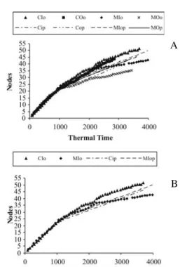
Visibly, there were two segments in the relationship of nodes number vs. thermal time, each one with a different slope. Figure 1 shows node numbers on the main stem of Cape
gooseberry as a function of days after transplanting and Figure 2 shows node numbers vs. thermal time (TT, oCd). When thermal
time was used as the independent variable, greater homogeneity was found in the number of nodes, especially in the initial segment. The first segment of the number of nodes vs. oCd took
place until cumulative thermal time was estimated to be 1039.5
oCd (degrees days). The criterion used to determine the time at
which the slope changed was minimum mean square error of (simulated – observed) node numbers.
The estimated parameters, standard errors and confidence limits (95%) are shown in Table 1. The rates of node appearance from the first and second segments were significantly different. Over a time period of one thousand degree days, twenty three nodes were formed in the first segment; in contrast, after that only eight nodes were formed in the second segment. A Student t-test was used to verify that the average residuals were statistically equal to zero in both segments (Pr >|t|=1). The
normality distribution test of Shapiro-Wilks (Pr < W 0.2617) confirmed that the residuals followed the normal distribution for the first segment. However, the distribution of residuals for the second segment was not normal. Furthermore, the variances were homogeneus in either case. In the first segment, the average rate of node appearance was 0.02 nodes (oCd)-1 and in the second
one, average rate decreased to 0.008 nodes (oCd)-1.
The rate of node appearance in plants of the Australian commercial sugarcane varieties Q117 and Q138 in a controlled environment at temperatures of 14, 18, 22 and 26oC was
significantly correlated with the temperature (Campbell et al. 1998). Analysis of the varietal rates of node deposition as a function of time allowed determination of both base temperature for node (hence leaf) appearance and phyllochron. The base temperatures for node appearance were 7.8 oC for Q117 and 7.6 oC for Q138.
In tomato, Scholberg et al. (2000) found that the maximum rate of main-stem node development was near 0.5 nodes per day and by the time of transplant plants, the number of nodes was between 3.1 and 6.3. The initial flowering happened approximately 4 weeks after transplanting when there was a total of 8-10 nodes in the main stem. The initial rate of nodes was 0.027 nodes oCd
(cumulative degrees days were less than 530 oCd), assuming a
base temperature of 10 oC and a maximum node development rate
at 28 oC. In terms of days, the average node-development rate
was 0.49 nodes/day, similar to 0.5 nodes/day for greenhouse tomato found by Jones et al. (1989). Main-stem node formation typically stopped increasing appreciably (tailed off) after the accumulation of 530 oC and the formation of 15.7 nodes. The
total maximum number of main-stem nodes ranged from 19 to 21. In Lucerne, Moot et al. (2001) and Brown and Moot (2004) found that node appearance was faster in the spring and in the summer than in the winter. They worked with a base temperature for thermal time accumulation of 1 oC when air temperatures were
below 15 oC and with a base temperature of 5 oC for temperatures
higher than 15 oC. The response for nodes appearance was linear
Reddy and Pachepsky (2002) studied, under controlled conditions and on the field, the effects of the temperature on the main stem node appearance in cotton. They concluded that these kinds of studies are valuable, contributing information for appropriate control and management of crop cultivation.
Simulation of node appearance
The empirical non-linear segmented model used to estimate the base temperature can also be used to simulate nodes vs. time in variable temperature conditions. Hesketh et al. (1973), Yan and Hunt (1999), Yin et al. (1995), Kim and Reddy (2004) and Setiyono et al. (2005) applied a non-linear model of development vs. temperature to describe and simulate the phenological behavior of diverse cultivations.
Minimum and maximum rates of node appearance were greater in Miraflores than in Chia and the lowest rate was reached for higher temperatures. The duration, in terms of thermal time and in days after transplanting (DAT), and the number of nodes responded similarly to temperature (Table 2). It is interesting to observe how in Chia out (field-grown plants) and Miraflores in (greenhouse-grown plants), the lowest rate of node appeareance was reached later than those grown in the other conditions. However, the highest rate was reached earlier in Chia out than in the others. As a result, Chia out showed a shorter duration between the minimum and the maximum rate of node appearance, but the number of nodes was greater by the time the minimum rate was reached. However, in total plants in Chia out showed fewer numbers of nodes.
The resulting equations for node appearance simulation applying Euler’s method were respectively for the first and second phase:
Node1t = Node1,t-1+ { 0.023 ( Tt - 6.29 )} (5) Node2t =Node2,t-1+{0.008 (Tt - 6.29 )} when TT > 1039.5 oCd (6)
The intercept was estimated as 0.702 nodes, which was used as node initial value to begin the simulation. Figures 1 and 2 show the number of observed and simulated nodes as functions of days after transplant and of thermal time for the locations under greenhouse and open field conditions respectively. For the first segment, the simulated values were more accurately predicted than those of the second segment. The appearance of nodes was less variable during the first segment, which corresponds to the vegetative phase of the plant. During the second phase, fruits were grown and harvested, which may result in competition for new node formation due to source-sink relationships.
Other authors have not considered the base temperature in their models, for example, in soybean Setiyono et al. (2005) used two functions to estimate the rate of node appearance, one in terms of temperature, different from thermal time, and another with chronological time that relates to the decrease of the rate for nodes appearance. The simulation with both functions fit the data satisfactorily. On the other hand, Hesketh et al. (1973) determined that vegetative development was sensitive to temperature and found a linear relationship between rate of node formation and temperature. Yan and Hunt (1999) simulated relative rates of growth as a function of the minimum, maximum and optimum temperatures in order to determine the phenology, adaptation and yield of corn, bean, sorghum, and wheat among other crops. The applied model successfully described the phenology of the cultures previously mentioned. Kim and Reddy (2004) developed a simple corn simulation model, in which they used the beta function, applied in other models by Yin et al. (1995). The rate of growth was expressed in terms of mean air temperature, optimum temperature at which the maximum rate of development was reached and the base temperature at which the development ceases. These models do not permit to estimate the duration of each phenological stage, in terms of thermal time or accumulated energy.
Parameter Estimate Standard error Lower limit 95% Higher limit 95% R2
a1 0.023 0.00056 0.4513 0.96400 0.9046
b 0.702 0.12570 0.0212 0.02340
Tb 6.296 0.22070 5.8548 6.73770
a2 0.008 0.00044 0.0074 0.00926 0.7100
TABLE 1 - Parameters estimated for node appearance model.
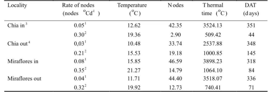
Locality Rate of nodes
(nodes oCd-1 )
Temperature (oC )
N odes T hermal
time (oC )
DAT (d ays)
0.051 12.62 42.35 3524.13 351
Chia in3
0.302 19.36 2.90 509.42 44
0,031 10.48 33.74 2537.88 348
Chia out4
0.212 15.53 19.18 1000.85 145
0.081 15.85 46.59 3898.23 318
Miraflores in
0.352 21.27 14.79 1064.10 84
0.041 11.71 44.40 3518.07 336
Miraflores out
0.322 19.92 12.73 740.41 71
TABLE 2 - Minimum1 and maximum2 rate of nodes appearance, duration and number of nodes.
CONCLUSIONS
It was possible to model the node appearance as segmented non-linear functions of thermal time. The empirical segmented model proposed for the first segment provided a basis for estimating the base temperature for node appearance and also was useful for estimating the slopes of the vegetative and reproductive phases. The base temperature (Tb) for node appearance was estimated as 6.29 oC required for computing
thermal time (TT). The estimated parameters and thermal time allowed established the simulation model for node appearance. The simulation of the first segment, the vegetative stage, predicted with more accuracy than the second one possibly due to multiple processes which were present in the reproductive stage. The model was relatively successful for all locations (RSME=2.10). The proposed model can be used to simulate nodes appearance for any other conditions just having the daily average temperature.
REFERENCES
ANGULO, R. Frutales exóticos de clima frío. Bogotá: Bayer CropScience, 2003. p.27-48.
ANGULO, R. (Ed.). Uchuva el cultivo. Bogotá: Universidad Jorge Tadeo Lozano, Centro de Investigaciones y Asesorias Agroindustriales, 2005. 78p.
BAKER, J.; REDDY, V. Temperature effects on phenological development and yield of muskmelon. Annals of Botany, London, v.87, p.605-613, 2001.
BROWN, H.E.; MOOT, D.J. Main-stem node appearance of lucerne regrowth in a temperate climate. In: INTERNATIONAL CROP SCIENCE CONGRESS, 14., 2004. Brisbane, Australia.
Proceedings… 2004. Available in: <http:// www.cropscience.org.au/icsc2004/poster/ 2/8/1939_brown.htm>. Access in: 22 nov. 2006.
CAMPBELL, J.A.; ROBERTSON, M.J.; GROF, C.P.L. Temperature effects on node appearance in sugarcane. Australian Journal of Plant Physiology, Collingwood,v.25, n.7, p.815-818, 1998.
COOMAN, A. Feasibility of protected tomato cropping in the high altitude tropics using statistical and system dynamic models for plant growth and development. Thesis (PhD) - Katholieke Universiteit Leuven, Faculteit Landbowkundige en Toegespaste, Biologische Weterischappen, Leuven, Belgium, 2002.
ELLIS, R. H.; WATKINSON, A. R.; SUMMERFIELD, R. J.; LAWN, R.J. From evaluation descriptors of times to flowering to the genetic characterization of flowering responses to fotoperiod and temperature. Plant Genetic Resources Newsletter, Maccarese, n.103, p.36-38, 1995.
A
B
FIGURE 1-(A) Node appearance vs. thermal time (TT, oCd). COo,
CIo, MOo, MIo are the observed nodes and COp, CIp, MOp, MIp are the predicted nodes for Chia and Miraflores in an open field and inside the greenhouse respectively. (B) - Node appearance
vs. thermal time for locations inside the greenhouse.
FIGURE 2 -(A) Node appearance vs. days after transplanting.
COo, CIo, MOo, MIo are the observed nodes and COp, CIp, MOp, MIp are the predicted nodes for Chia and Miraflores in an open field and inside the greenhouse respectively.(B) - Node appearance
vs. days after transplanting for locations inside the greenhouse.
A
FAO. Fruit-bearing forest trees technical notes. Rome: Food
and Agriculture Organization of the United Nations, 1982. p.140-143.
FISCHER, G.; EBERT, G.; LÜDDERS, P. Production, seeds and carbohydrate contents of Cape gooseberry (Physalis peruviana L.) fruits grown at two contrasting Colombian altitudes. Journal of Applied Botany and Food Quality, Göttingen, v.81, p.29-35,
2007.
FISCHER, G. Crecimiento y desarrollo. In: FLOREZ, V.J.; FISCHER, G.; SORA, A.D. (Ed.). Producción, poscosecha y exportación de la uchuva Physalis peruviana L. Bogotá: Unibiblos, Universidad
Nacional de Colombia, 2000. p.9-26.
HESKETH, J.D.; MYHRE, D.L.; WILLEY, C.R. Temperature control of time intervals between vegetative and reproductive events in soybeans. Crop Science, Madison, v.13, p.250-254, 1973.
JONES, J.W.; DAYAN, E.; VAN KEULAN, H.; CHALLA, H. Modeling tomato growth for optimizing greenhouse temperatures and carbon dioxide concentrations. Acta Horticulturae,
Wageningen, v.248, p.285-294, 1989.
JONES, J.W.; LUTEN, J.C. Simulation of biological processes. In: PEART, M.; ROBERT, M.; CURRY, B.R. (Ed.). Agricultural systems modeling and simulation. New York: Marcel Dekker
Publishers, 1998.
KEEN, R.E.; SPAIN, J.D. Computer simulation in biology: a BASIC introduction. New York: Wiley-Liss, . 1992. 498p.
KIM, S.H.; REDDY, V..Simulating maize development using a nonlinear temperature response model. In: INTERNATIONAL CROP SCIENCE CONGRESS, 4., 2004, Brisbane, Australia.
Proceedings…
LEGGE, A.P. Notes on the history, cultivation and uses of Physalis peruviana L. Journal of the Royal Horticultural Society,
London, v.99, n.7, p.310-314, 1974.
MILLER, P.: LANIER, W.; BRANDT, S. Montguide MT20013 AG 7/2001. Bozeman, MT: Montana State University, Extension
Service, 2001.
MOOT, D.J.; ROBERTSON, M.J.; POLLOCK, K.M.Validation of the APSIM-Lucerne model for phenological development in a cool-temperate climate. In: AUSTRALIAN AGRONOMY
CONFERENCE, 10., 2001. Hobart, Tasmania, Australia.
Proceedings… 2001. Available: <http://www.regional.org.au/au/
asa/2001/6/d/moot.htm>. Access in: 15 jan. 2007.
ORTEGA, S.O.; LOZANO, P.; MORENO, Y.; LEÓN, L. Desarrollo de modelos predictivos de fenología y evolución de madurez en vid para vino cv. Cabernet Sauvignon y Chardonnay. Agricultura Técnica,Chile, v.62, n.1, p.27 -37, 2002.
REDDY, V.; PACHEPSKY, Y.A. Temperature effects on node development rates in cotton. Annals of Botany, London, v.31,
p.101-111, 2002.
ROBERTSON, M.J.; CARBERRY, P.S.; HUTH, N.I.; TURPIN, J.E.; PROBERT, M.E.; POULTON, P.L.; BELL, M.; WRIGHT, G.C.; YEATES, S.J.; BRINSMEAD, R.B. Simulation of growth and development of diverse legume species in APSIM. Australian Journal of Agricultural Research, Collingwood, v.53, p.429-446,
2002.
ROCHE, R.; JEUFFROY, M.H.; NEY, B. A model to simulate the final number of reproductive nodes in pea (Pisum sativum L.).
Annals of Botany, London. v.81, p.545-555, 1998.
SALAZAR, M.R. Un modelo simple de producción potencial de uchuva (Physalis peruviana L.). 2006. Thesis (PhD) - Facultad de Agronomía, Universidad Nacional de Colombia, Bogotá, 2006.
SCHOLBERG, J.; MCNEAL, B.L.; JONES, J.W.; BOOTE, K.J.; STANLEY, C.D.; OBREZA, T.A. Growth and canopy
characteristics of field-grown tomato. Agronomy Journal,
Madison, 92, p.152–159, 2000.
SETIYONO, T.; DOBERMANN, A.; WEISS, A.; SPECHT, J.; BASTIDAS, A. Soybean phenology: Simulating node-appearance (V-stages) using non-linear temperature and chronological function related to reproductive stage. In: ASA-CSSA-SSSAINTERNATIONAL ANNUAL MEETINGS, 2005. . Proceedings… Lincoln: University of Nebraska, 2005.
SCHWARTZ, M. D. Advancing to full bloom: planning phonological research for the 21st century. International Journal of Biometeorology, New York, v.42, p.113-118, 1999.
THORNLEY, J.H.M.; JOHNSON, H.R. Plant and crop modelling.
Oxford: Clarendon Press, 1990.
TORRES, E. Agrometeorologia. México, DF: Editorial Trillas, 1995.
154 p.
VERGHIS, T.I.; MCKENZIE, B.A.; HILL, G.D. Phenological development of chickpeas (Cicer arietinum) in Canterbury, New Zealand. New Zealand Journal of Crop and Horticultural Science, Wellington, v.27, p.249-256, 1999.
VIATOR, R.P.; NUTI, R.C.; EDMISTEN, K.; WELLS, R. Predicting cotton boll maturation period using degree days and other climatic factors. Agronomy Journal, Madison, v.97, p.494-499, 2005.
WILLIAMS, D.W.; ANDRIS, H.L.; BEEDE, R.H.; LUVISI, D.A.; NORTON, M.V.K.; WILLIAMS, L.E. Validation of a model for the growth and development of the Thompson Seedless grapevine. II. Phenology. American Journal of Enology and Viticulture,
Davis, v.36, p.283-289, 1985.
YAN, W.; HUNT, L.A. An equation for modelling the temperature response of plants using only the cardinal temperatures. Annals of Botany, London, v.84, p.607-614, 1999.
YIN, X.; KROPFF, M.J.; MCLAREN, G.; VISPERAS, R.M. A nonlinear model for crop development as a function of temperature. Agricultural and Forest Meteorology, Amsterdam,