Gabriel Araújo e Silva Ferraz1, Marcelo Silva de Oliveira2, Fábio Moreira da Silva3, Ronan Souza Sales4, Luis Carlos Cirilo Carvalho5
(Received: February 3, 2017; accepted: Friday, May 12, 2017)
ABSTRACT: The aim of the present study was to evaluate different grid samples applied to plant properties of a coffee plantation by using precision coffee growing and geostatistical techniques. The study was performed at the Brejão Farm in the municipality of Três Pontas, MG, Brazil, using productivity, the maturation index and the detachment force difference, sampled at georeferenced points. With the intention of choosing an optimum grid, 20 grid samples were tested through semivariogram fitting and validation tests seeking to combine the accuracy and precision that the grid sample can present through an optimal grid indicator, allowing choosing a more suitable grid. It was possible to characterize the magnitude of the spatial variability of plant properties under study in all the proposed grids. The grid that best represented the three variables under study was the grid with 64 sample points in squared grid and nine zoom grid points. The proposed methodology for the present study allowed observing the difference among different grid samples and among the variables of plant productivity, maturity index and detachment force.
Index terms: Precision agriculture, geostatistics, coffee tree, spatial variability.
DETERMINAÇÃO DE MALHAS AMOSTRAIS DA PLANTA EM CAFEICULTURA DE PRECISÃO
RESUMO: O objetivo do presente trabalho foi estudar diferentes grades amostrais aplicadas aos atributos da planta de uma lavoura cafeeira por meio do uso da cafeicultura de precisão e das técnicas geoestatísticas. O trabalho foi realizado na fazenda Brejão no município de Três Pontas - MG, utilizando-se a produtividade, o Índice de Maturação e a Diferença da Força de Desprendimento, amostrados em pontos georreferenciados. Para que pudesse ser escolhida uma grade ótima, foram testadas 20 grades amostrais, por meio do ajuste de semivariogramas e testes por validação, buscando aliar a exatidão e a precisão que a grade amostral pode apresentar por meio de um indicador de grade ótima, o que permite a escolha de uma grade mais adequada. Foi possível caracterizar a magnitude da variabilidade espacial dos atributos da planta em estudo em todas as grades propostas. A grade que melhor representou as três variáveis em estudo foi a grade com 64 pontos amostrais em malha quadrada e 9 pontos de grade zoom. A metodologia proposta por este trabalho permitiu observar a diferença existente entre as diferentes grades amostrais e também entre as variáveis da planta produtividade, índice de maturação e força de desprendimento
Termos para indexação: Agricultura de Precisão, geostatistica, cafeeiro, variabilidade espacial.
1 INTRODUCTION
According to Ferraz et al. (2012c), the precision agriculture of the coffee growing has been termed as precision coffee growing, being define by the authors as a set of techniques and technologies capable of assisting the coffee farmer to manage the crop, based on the spatial variability of soil and plant properties, in order to maximize profitability, increase efficiency of fertilization, spraying and harvesting, thus increasing productivity and the product’s final quality. Additionally, according to Ferraz et al. (2011), precision coffee growing may be an economically viable technique for producers.
1,3Federal University of Lavras/ULFA - Department of Engineering/DEG - 37.200-000 - Lavras - MG - gabriel.ferraz@ufla.
2Federal University of Lavras/UFLA - Department of Exact Sciences/DEX - 37.200-000 - Lavras - MG - [email protected] 4University Center of Formiga/UNIFOR - Avenida Doutor Arnaldo de Senna, n°328 - Água Vermelha - 35.570-000 - Formiga- MG
5State University of Santa Cruz/UESC - Department of Agricultural and Environmental Sciences - 45.662-900 - Ilhéus - BA
It is known that the coffee cultivation in Brazil occurs within a diversity of factors that can strongly influence the coffee productivity and the crop management homogeneously and lead to a reduced profitability to the rural producer. In this respect, spatial analyses of productivity tend to provide a more efficient management of the production process (ALVES et al., 2009). Based on spatial variability maps of productivity, the producers can identify crop areas where productivity can be improved or require adjustments in the fertilizer recommendation in order to optimize the income of the property (PIERCE et al., 1997).
64 georeferenced sample points (2.9 points per hectare) using topographic GPS. Within this regular grid sampling, another four regular grid samples of 3.8 x 3.8 m were created, called zoom, which were positioned at four points of the main grid. Each zoom will correspond to 10 georeferenced sample points (one point of the main grid and nine of the new grid). Thus, the initial grid sampling consisted of 100 georeferenced points (Figure 1a).
Each sampling point corresponds to four plants: two located in the coffee line where the point was georeferenced and the other two in each lateral line to the reference point.
The use of zoom grids aims to detect variations in small distances, collaborating to reduce the nugget effect and hence contributing to improve the used grid. This type of sampling using smaller grids (zoom) within a larger grid was also used in the studies of Gontijo et al. (2007) and Sampaio et al. (2010).
Based on the initial grid, another 19 grids were created (Table 1 and Figure 1). The grids were grouped into four groups that were based on base grids. In Group 1, the base grid had 64 georeferenced sample points (2.9 points per hectare) (grid 5); in Group 2, the base grid had 46 points (2.09 pt/ha) (grid 10); in Group 3, the base grid had 23 points (1.04 pt/ha) (grid 15); and the Group 4, the base grid had 12 georeferenced sample points (0.54 pt/ha) (grid 20).
The initial grid of each group consists of the base grid plus four zoom grids. The second grid of each group consists of the initial grid of the group removing the grid that is in the southeast portion of the area. The third grid is characterized by the second grid of the group removing the zoom grid of the northwest portion of the area. To form the fourth grid, the third grid was used removing the zoom grid in the northeast portion of the area. The fifth grid is characterized only by the base grid (Figure 1). Three properties related to the plant were collected: productivity, MI and fruit detachment force. The collection of coffee plant properties such as productivity, MI and detachment force was performed in 2011.
from 75 to 80%), 10 to 15% green fruits represent the middle of the harvest (MI from 85 to 90%) and less than 5% for the end of the harvest (MI of 95%). Silva (2008) observed that the detachment force of green fruits was 73% higher than the cherry fruits, and that this difference could be a relevant factor for the selective mechanized harvest of coffee fruits. Thereby, the study on the spatial variability of the MI and the detachment force of coffee fruits allied to the productivity study may be extremely important for a better mechanized harvesting operation.
Spatial variability is one of the premises for the application of precision coffee growing and its identification is very difficult for farmers. The use of grid samples allows the coffee grower observing this variability, but the use of grids with unsatisfactory size can generate maps that do not reflect the field and therefore generating erroneous recommendations, which may cause losses to the producers. Thus, the study of grid samples becomes highly relevant for the more precise management of the spatial variability of plant properties in a coffee plantation, particularly aiming the mechanized harvest.
The aim of the present study was to evaluate different grid samples applied to the plant properties (productivity, MI and detachment force) of a coffee plantation using precision coffee growing and geostatistical techniques in order to find a grid sample best fitted to the variables under study.
2 MATERIAL AND METHODS
The experiment was developed at the Brejão Farm, in the municipality of Três Pontas, southern of the state of Minas Gerais, Brazil, in an area of 22 ha of coffee (Coffea arabica L.) cv. Topázio transplanted in December 2005 at a spacing of 3.8 m between the lines and 0.8 m between plants, totaling 3289 plants.ha-1. The geographic coordinates of the center point of the area are 21°25’58” S and 45°24’51” WGr. The limit points of the area were obtained using topographic GPS (mean error of 10 cm).
The coffee productivity (L.plant-1) was obtained by manual harvesting on cloths of the four plants around the sampling point, and the volume harvested from each plant, after cleaning, was measured in a graduated container in liters. After this measurement, the average yield of these four plants was obtained, resulting in the productivity value for the sampling point.
At each sampling point, after the
productivity measurements, the harvested
fruits from the four plants were placed in
FIGURE 1 - Grid sampling tested in the study area.
the same container, being homogenized to
take a 0.5 L sample of fruits (CARVALhO
et al., 2003; SILVA,
2008). Based on this volume, the fruit counting was performed for each ripeness stage (dry, raisin, cherry and green) and transformed them as percentage so that the equation (Maturation Index) described by Alves et al. (2009) could be used:1 3 64 2 18 82 4 64 1 9 73 5 64 0 0 64 2 6 46 4 36 82 7 46 3 27 73 8 46 2 18 64 9 46 1 9 55 10 46 0 0 46 3 11 23 4 39 62 12 23 3 30 53 13 23 2 20 43 14 23 1 10 33 15 23 0 0 23 4 16 12 4 40 52 17 12 3 30 42 18 12 2 20 32 19 12 1 10 22 20 12 0 0 12
In order to obtain the fruit detachment force (DF) data, five fruits were collected (two from the upper third, one from the middle third and two from the lower third), according to the methodology proposed by Ferraz et al. (2017), for each ripeness stage (green and cherry) at every plant from the sampling point. After collecting these fruits, the average of the detachment force of the four plants was obtained for each ripeness stage.
The determination of this detachment force was performed through a portable digital dynamometer model DD-500 manufactured by Instrutherm Instrumentos de Medição Ltda. that offers measurements in Newton.
After obtaining the green fruit detachment force (GDF) and the cherry fruit detachment force (CDF), the detachment force difference (DFD) was obtained as follows:
DFD = GDF - CDF
The spatial dependence of plant properties of the coffee plantation were analyzed by semivariogram fitting, estimated as follows:
( )
N(h)[
( ) (
)
]
2 1 i i i h x z x z ) h ( N 2 1 h ˆ∑
= + − = γwhere N (h) is the number of experimental pairs of observations z(xi) and z (xi + h) separated by a distance h. The semivariogram is represented by the graph γˆ h( ) versus h. From the fit of a
mathematical model to the calculated values of
) ( ˆ h
γ , the coefficients of the theoretical model
were estimated for the semivariogram called nugget effect (C0); sill (C0+C1); and range (a), as described by Bachmaier and Backers (2008).
The ordinary least squares (OLS) method and the spherical model were used for all the studied variables and for all the tested grids. According to Webster and Oliver (2007), the spherical mathematical model is most often
used in geostatistics. This model is widely used on spatial variability studies in coffee crops of soil properties, productivity, defoliation, fruit detachment force and pest infestation (ALVES et al., 2009; FERRAz et al., 2012b; MOLIN et al., 2010; SILVA et al., 2007, 2008; SILVA, A. et al., 2010; SILVA, F. C. et al., 2010).
The spatial dependence degree of properties under study were analyzed through the classification of Cambardella et al. (1994), in which semivariograms with strong spatial dependence show a nugget effect < 25% sill, moderate between 25 and 75% and weak > 75%.
According to Isaaks and Srivastava (1989), validation is the error estimation technique that allows comparing predicted values with the sampled ones. The sample value, at a certain location z(si), is temporarily discarded from the data set, and then a (ordinary) kriging prediction is performed on the location Zˆ
( )
s( )i , using theremaining samples. Thereby, it is possible to extract some values that will be very useful for observing the errors presented by each grid, such as absolute error (AE), standard deviation of absolute error (SDAE).
The selection criteria based on cross-validation should find the AE value closer to zero and the value of SDAE as lower as possible. These criteria can be obtained by using the following expressions:
where: n is the data number; z(si) is the value observed at point si; and zˆ
( )
s(i) is the value predicted by ordinary kriging at point si, excluding the observation Z(si).The AE value reflects the accuracy of the grid sample, since the accuracy gives conceptually an idea of the conformity degree of a measured or calculated value in relation to a standard reference. The AE compares the values obtained by validation with the actual values obtained by the field samplings. In order to be able to find an accuracy component that would allow comparing among the grids, the accuracy index (AI) was developed.
The AI is given by the AE value of the grid, in module, divided by the largest value, in module, of the absolute error (mAE) presented by the analyzed grids.
On the other hand, the value of the SDAE reflects the grid accuracy, where by definition the accuracy is used to express the dispersion of results. Moreover, the precision index (PI) was developed to compare the accuracy component of the grid among the different studied grids.
The PI is given by the value of SDAE of the grid divided by the highest value of the standard deviation of absolute error (mSDAE) presented by the group of analyzed grids.
In order to select the best grid sampling (optimum grid) among the 20 studied grids, the optimum grid indicator (OGI) was created, which considers both AI and PI. The OGI is given by:
The OGI ranges from zero to one, being that the closer the zero, the better the grid (more accurate and more precise), while the closer to one, the worse (the more inaccurate and imprecise) is the grid.
The data was tabulated in electronic spreadsheets. For the geostatistical analysis, the R statistical software was used, through the geoR package (RIBEIRO JUNIOR; DIGGLE, 2001).
3 RESULTS AND DISCUSSION
Based on the geostatistical analysis methodology, it was possible to quantify the magnitude and structure of spatial dependence of productivity (Prod), Maturation Index (MI) and the detachment force difference (DFD) and in all the grids under study (Table 2). The absolute value of the difference between two observed samples increased when the samples distanced away until a value in which the locality no longer influenced, resulting in the stability of the experimental semivariogram from the distance separating the structured variability from the random one.
The nugget effect is an important parameter of the semivariogram and indicates unexplained variability, considering the sampling distance used. For the Prod variable, the nugget effect ranged from 0 (grid 10 and 15) to 1.84 (grid 3) (Table 2). The MI ranged from 43.38 (grid 20) to 353.13 (grid 4) (Table 2). For the DFD, the nugget effect ranged from 0 (grid 19 and 20) to 0.64 (grid 12) (Table 2).
1 100 285 1.40 0.44 1.84 125.74 76.19 Weak 0.0011 1.33 0.0655 0.8165 0.4410 2 91 290 1.14 0.90 2.04 241.28 56.10 Mod 0.0042 1.34 0.2482 0.8212 0.5347 3 82 390 1.84 0.31 2.14 354.63 85.58 Weak 0.0032 1.39 0.1867 0.8532 0.5199 4 73 300 1.05 1.08 2.13 287.61 49.35 Mod 0.0042 1.29 0.2453 0.7919 0.5186 5 64 290 1.20 1.00 2.19 261.53 54.54 Mod 0.0036 1.31 0.2091 0.7993 0.5042 6 82 243 1.50 0.40 1.90 113.24 79.03 Weak 0.0017 1.36 0.0995 0.8296 0.4645 7 73 243 1.60 0.50 2.10 272.18 76.19 Weak 0.0050 1.39 0.2929 0.8521 0.5725 8 64 300 1.58 0.65 2.23 274.94 70.72 Mod 0.0066 1.46 0.3883 0.8903 0.6393 9 55 243 0.83 1.20 2.03 214.99 40.98 Mod 0.0121 1.39 0.7078 0.8513 0.7796 10 46 243 0.00 2.14 2.14 165.34 0.00 Str 0.0121 1.39 0.7078 0.8513 0.7796 11 62 223 1.00 0.93 1.93 130.08 51.82 Mod -0.0001 1.40 0.0041 0.8570 0.4306 12 52 223 1.13 0.93 2.06 178.36 54.74 Mod 0.0027 1.49 0.1608 0.9114 0.5361 13 42 223 1.28 1.30 2.58 216.09 49.71 Mod 0.0028 1.63 0.1612 1.0000 0.5806 14 32 223 0.75 1.45 2.20 175.96 34.03 Mod 0.0095 1.47 0.5585 0.9021 0.7303 15 23 223 0.00 2.64 2.64 117.98 0.00 Str 0.0107 1.50 0.6259 0.9148 0.7703 16 52 223 1.13 0.56 1.69 129.02 66.73 Mod 0.0125 1.34 0.7307 0.8221 0.7764 17 42 223 1.24 0.63 1.86 134.95 66.34 Mod 0.0114 1.45 0.6680 0.8896 0.7788 18 32 220 1.39 0.66 2.05 148.24 67.84 Mod 0.0158 1.60 0.9233 0.9775 0.9504 19 22 223 0.75 1.07 1.82 137.61 41.34 Mod 0.0171 1.45 1.0000 0.8850 0.9425 20 12 223 0.53 1.53 2.05 100.00 25.65 Mod 0.0000 1.61 0.0000 0.9864 0.4932
Maturation index (MI)
1 100 370 191.96 234.37 426.33 295.26 45.03 Mod -0.1127 15.66 0.2185 0.8206 0.5196 2 91 283 211.49 176.96 388.45 271.66 54.44 Mod -0.0733 15.98 0.1420 0.8373 0.4897 3 82 283 262.73 142.68 405.40 299.73 64.81 Mod -0.0263 16.78 0.0510 0.8792 0.4651 4 73 390 353.13 237.11 590.23 353.13 59.83 Mod -0.0013 16.09 0.0026 0.8427 0.4226 5 64 390 107.21 301.17 408.38 322.85 26.25 Mod -0.0928 14.79 0.1800 0.7750 0.4775 6 82 280 198.75 149.90 348.65 242.12 57.00 Mod -0.0968 15.18 0.1877 0.7955 0.4916 7 73 280 225.07 100.66 325.73 268.52 69.10 Mod -0.0109 15.34 0.0212 0.8035 0.4124 8 64 310 288.28 17.60 305.88 257.11 94.24 Weak 0.0177 16.79 0.0343 0.8795 0.4569 9 55 290 273.53 22.61 296.13 264.77 92.37 Weak 0.0370 15.80 0.0717 0.8279 0.4498 10 46 248 99.50 146.96 246.45 234.36 40.37 Mod -0.0175 14.16 0.0339 0.7418 0.3879 11 62 260 178.15 200.91 379.05 245.93 47.00 Mod -0.1451 16.22 0.2814 0.8496 0.5655 12 52 280 186.45 187.32 373.77 248.62 49.88 Mod -0.0170 16.76 0.0330 0.8782 0.4556 13 42 280 295.46 99.73 395.19 252.25 74.76 Mod 0.0905 18.35 0.1755 0.9615 0.5685 14 32 260 273.56 120.49 394.06 213.02 69.42 Mod 0.1565 17.42 0.3035 0.9127 0.6081 15 23 260 126.51 159.82 286.34 225.94 44.18 Mod -0.2860 16.30 0.5546 0.8537 0.7041
Once it is impossible to quantify the individual contribution of these errors, the nugget effect can be expressed as sill ratio, thus facilitating the comparison of the of spatial dependence degree (DD) of the study variables (TRANGMAR; YOST, UEHARA, 1985). Through the classification of Cambardella et al. (1994), the Prod variable can be classified as a strong spatial dependence degree for two grids (grids 10 and 15), moderate for 14 grids and weak for four grids (grids 1, 3, 6 and 7). The MI variable showed moderate DD for 18 grids and only two grids showed weak DD (grids 8 and 9). For the DFD, five grids showed strong DD (grids 10, 14, 15, 19 and 20), nine with moderate DD and six with weak DD (grids 1, 2, 3, 6, 7 and 8).
The range values for semivariograms are highly relevant in determining the spatial
16 52 270 123.62 268.52 392.14 246.69 31.52 Mod 0.0670 16.51 0.1300 0.8651 0.4975 17 42 270 163.91 204.19 368.10 258.15 44.53 Mod 0.2214 17.25 0.4293 0.9035 0.6664 18 32 270 257.82 149.69 407.51 230.62 63.27 Mod 0.3997 19.09 0.7751 1.0000 0.8875 19 22 280 255.15 98.34 353.49 240.07 72.18 Mod 0.5157 17.82 1.0000 0.9337 0.9669 20 12 280 44.38 132.71 177.09 115.53 25.06 Mod 0.0001 14.82 0.0001 0.7764 0.3883
Detachment force difference (DFD)
1 100 340 0.55 0.16 0.71 250.92 77.50 Weak 0.0017 0.7166 0.0235 0.7729 0.3982 2 91 340 0.63 0.11 0.74 261.73 85.10 Weak 0.0010 0.7376 0.0144 0.7955 0.4050 3 82 350 0.62 0.10 0.72 279.04 85.53 Weak 0.0001 0.7257 0.0008 0.7827 0.3918 4 73 380 0.44 0.22 0.66 135.82 66.31 Mod 0.0058 0.6916 0.0799 0.7459 0.4129 5 64 300 0.22 0.44 0.65 193.70 33.15 Mod -0.0036 0.6603 0.0497 0.7121 0.3809 6 82 320 0.63 0.12 0.75 242.28 83.64 Weak 0.0034 0.7477 0.0472 0.8064 0.4268 7 73 320 0.70 0.09 0.79 260.00 88.29 Weak 0.0028 0.7738 0.0387 0.8345 0.4366 8 64 350 0.63 0.13 0.76 216.17 83.52 Weak 0.0025 0.7481 0.0339 0.8068 0.4204 9 55 390 0.34 0.34 0.69 75.27 50.02 Mod 0.0133 0.7573 0.1832 0.8168 0.5000 10 46 250 0.07 0.59 0.66 128.01 10.30 Str 0.0012 0.7099 0.0164 0.7656 0.3910 11 62 360 0.55 0.22 0.77 188.38 71.77 Mod 0.0108 0.7638 0.1490 0.8237 0.4864 12 52 360 0.64 0.22 0.85 227.93 74.47 Mod 0.0098 0.7986 0.1349 0.8613 0.4981 13 42 290 0.52 0.45 0.97 254.62 53.85 Mod 0.0100 0.7865 0.1372 0.8483 0.4928 14 32 240 0.00 1.19 1.19 39.93 0.07 Str 0.0521 0.8469 0.7173 0.9134 0.8154 15 23 240 0.11 0.70 0.81 168.76 13.49 Str 0.0099 0.8558 0.1362 0.9230 0.5296 16 52 260 0.38 0.51 0.89 71.61 42.61 Mod 0.0203 0.7966 0.2799 0.8591 0.5695 17 42 260 0.37 0.63 1.00 49.65 37.30 Mod 0.0265 0.8374 0.3658 0.9032 0.6345 18 32 260 0.31 0.84 1.16 70.07 27.07 Mod 0.0219 0.8283 0.3024 0.8933 0.5979 19 22 260 0.00 1.43 1.43 47.03 0.00 Str 0.0726 0.9272 1.0000 1.0000 1.0000 20 12 280 0.00 0.91 0.91 120.07 0.00 Str 0.0726 0.9272 1.0000 1.0000 1.0000
NPG - Number of points of the grid sampling; Max dist - Maximum distance used for semivariogram fitting; C0 - Nugget effect; C1 - Contribution; C0+C1 - Sill; a - range; DD - Spatial dependence degree; AE - Absolute error; SDAE - Standard error of absolute error; AI -
Accuracy index; PI - Precision index; OGI - Optimum grid indicator; Str - Strong; Mod - Moderate.
dependence threshold, which can also be indicative of the interval among soil mapping units (TRANGMAR; YOST; UEhARA, 1985) or properties related to plants (FERRAz et al., 2012c).
The studied variables showed different spatial dependence ranges, where the Prod had a range varying from 100 m (grid 20) to 354.63 m (grid 3) and the MI had its range varying from 115.53 m (grid 20) to 353.13 m (grid 4). For the DFD, the range varied from 39.93 m (grid 14) to 279.04 m (grid 3).
Ferraz et al. (2012a) studied productivity for three years and found range values equal to 217.24 m (2008), 280.51 m (2009) and 203.41 m (2010). Silva et al. (2008) studied two harvests and found range values equal to 65.04 m and 60.43 m, respectively,
fruits.
When testing the 20 grid samples for the DFD, the grid 5, with 64 sample points, showed the lowest OGI (0.3809), followed by the grids 10, 3, 1 and 2.
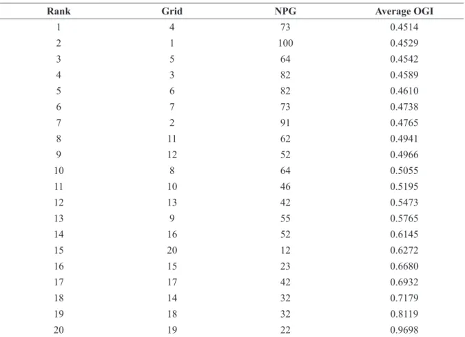
however, as can be noted, the management of mechanized and selective harvesting of coffee fruits involves both the productivity analysis and the MI and DFD, so that the harvesting process can be optimized. Therefore, these data should not be analyzed separately but rather as a whole in order to optimize and reduce the sampling and harvest operating costs. In order to proceed to the choice of the best grid sampling, it should start from the one that best fit the three variables under study. Thus, the average OGI was calculated, which is nothing more than the average OGI value showed by the three variables for each grid. In Table 3, the grids were classified according to the calculated average OGI values.
The grids 4, 1, 5, 3 and 6 showed the lowest average OGI values. In this list, the grid 5 is highlighted, with 64 sample points, 2.9 pt/ ha, without zoom grids, facilitating the sampling process. It was also noted a great influence of zoom grids, in which the grid samples that had this type of grid were superior the base grids of their groups.
According to Nanni et al. (2011) the grid samples used for soil sampling in the most diverse Brazilian cultures are around one point every 2 to 3 ha, being that, in some cultures, up to one point is used every 4 ha. The most commonly used grid sampling in coffee growing is one point per hectare (FERRAz et al., 2012c).
Whether only the base grids (grids 5, 10, 15 and 20) were tested, the grid 5 (2.9 pts/ha) would be highlighted, followed by grids 10 (2.09 pts/ha), grid 20 (approximately 0.5 pt/ha) and grid 15 (1.0 pt/ha).
Therefore, it can be observed that major errors would occur by using the wrong grid, being the correct choice of the grid sample of plant properties extremely important for the good management of the mechanized harvest.
grids under study, the validation criteria were used considering the AE and SDAE. For comparison purposes, the AI, PI, and an index that correlates the two OGI were created to choose the best grid.
For a good evaluation of the grid sampling, three plant properties were evaluated: Prod, MI and DFD.
Although a coffee harvester manufacturer has developed and launched a productivity sensor, used by Molin et al. (2010), this is not yet widespread and a good option to map the coffee crop productivity is performing the georeferencing of sampling points and manual harvesting of fruits, as proposed in the studies of Ferraz et al. (2012a, 2012b, 2012c), Silva et al. (2007, 2008) and Silva, F. M. et al. (2010), performed by the present study. Thus, it becomes important to analyze a grid sample that allows mapping the productivity in a coffee plantation harvested manually.
When performing the semivariogram fitting for every grid samples for the Prod variable and find the OGI, it can be noted that the grid that best fitted this variable (lower OGI) was the grid 11, whose value was 0.4305, with 62 sample points, followed by the grid 1 (OGI equal to 0.4409, with 100 sample points) and the grids 6, 20 and 5.
The MI is strongly widespread among coffee growers and this is one of the factors that indicate the harvesting time to the producer, especially the mechanized harvest, influencing even the number of passes that the harvester will perform in a certain area. Taking into consideration the importance of such index, the study on the spatial variability can reflect in the indication of more favorable locations to begin the harvest, besides indicating more precisely when to start the operation.
When observing the OGI for the MI variable, it can be observed that the grid 10, with 46 sample points, showed the lowest MI (0.3878). This was followed by the grids 20, 7, 4 and 9, respectively.
In the selective manual harvesting, coffee growers can choose which fruits should be collected, choosing those that are under optimal ripeness for harvesting. however, when the
4 CONCLUSIONS
It was possible to characterize the magnitude of the spatial variability of plant properties under study in all the proposed grids.
It was observed that the variables presented a spatial dependence structure, allowing obtaining the validation parameters.
Based on the methodology proposed in the present study, the grid that best suited the plant variables in order to optimize the harvesting operation was the grid 4, with 64 sampling points in the base grid plus nine zoom grid points, totaling 73 points.
5 REFERENCES
ALVES, M. C. et al. Geostatistical analysis of the spatial variation of the berry borer and leaf miner in a coffee agroecosystem. Precision Agriculture, Dordrecht, v. 10, n. 12, p. 1-14, Dec. 2009.
BAChMAIER, M.; BACKERS, M. Variogram or semivariogram?: understanding the variances in a variogram. Precision Agriculture, Dordrecht, v. 9, p. 173-175, Feb. 2008.
TABLE 3 - Ranking of grids based on average OGI
Rank Grid NPG Average OGI
1 4 73 0.4514 2 1 100 0.4529 3 5 64 0.4542 4 3 82 0.4589 5 6 82 0.4610 6 7 73 0.4738 7 2 91 0.4765 8 11 62 0.4941 9 12 52 0.4966 10 8 64 0.5055 11 10 46 0.5195 12 13 42 0.5473 13 9 55 0.5765 14 16 52 0.6145 15 20 12 0.6272 16 15 23 0.6680 17 17 42 0.6932 18 14 32 0.7179 19 18 32 0.8119 20 19 22 0.9698
CAMBARDELLA, C. A. et al. Field scale variability of soil properties in Central Iowa soils. Soil Science Society of America Journal, Madison, v. 58, n. 5, p. 1501-1511, 1994.
CARVALHO, G. R. et al. Eficiência do Ethephon na uniformização e antecipação da maturação de frutos de cafeeiro (Coffea arabica L.) e na qualidade da bebida. Ciência e Agrotecnologia, Lavras, v. 27, n. 1, p. 98-106, jan./fev. 2003.
FERRAz, G. A. S. et al. Agricultura de precisão no estudo de atributos químicos do solo e da produtividade de lavoura cafeeira. Coffee Science, Lavras, v. 7, n. 1, p. 59-67, jan./abr. 2012a.
______. Geostatistical analysis of fruit yield and detachment force in coffee. Precision Agriculture, Dordrecht, v. 13, n. 1, p. 76-89, Jan. 2012b.
______. Variabilidade espacial dos atributos da planta de uma lavoura cafeeira. Revista Ciência Agronômica, Fortaleza, v. 48, p. 81-91, 2017.
Engenharia Agrícola, Jaboticabal, v. 31, n. 5, p. 906-915, set./out. 2011.
GONTIJO, I. et al.Planejamento amostral da pressão de preconsolidação de um latossolo vermelho distroférrico. Revista Brasileira de Ciência do Solo, Viçosa, v. 31, p. 1245-1254, 2007.
ISAAKS, E. h.; SRIVASTAVA, R. M. An introduction to applied geostatistics. New York: Oxford University Press, 1989. 561 p.
JACINThO, J. L. et al. Management zones in coffee cultivation. Revista Brasileira de Engenharia Agrícola e Ambiental, Campina Grande, v. 21, p. 94-99, 2017.
MOLIN, J. P. et al. Teste procedure for variable rate fertilizer on coffee. Acta Scientiarum Agronomy, Maringá, v. 32, n. 4, p. 569-575, 2010.
NANNI, M. R. et al. Optimum size in grid soil sampling for variable rate application in site-specific management. Scientia Agricola, Piracicaba, v. 68, n. 3, p. 386-392, May/June 2011.
PIERCE, F. J. et al. Yield mapping. In: PIERCE, F. J.; SADLER, E. J. (Ed.). The state of site specific management for agriculture. Madson: ASA/CSSA/ SSA, 1997. p. 211-243.
RIBEIRO JUNIOR, P. J.; DIGGLE, P. J. GeoR: a package for geostatistical analysis. R-News,New York, v. 1, n. 2, p. 14-18, June 2001.
SÁ JUNIOR, A. et al. Application of the Köppen classification for climatic zoning in the state of Minas Gerais, Brazil. Theoretical and Applied Climatology, Wien, v. 108, p. 1-7, 2012.
Lavras, v. 5, n. 2, p. 173-182, maio/ago. 2010.
SILVA, F. C. Efeito da força de desprendimento e maturação dos frutos de cafeeiros na colheita mecanizada. 2008. 106 p. Dissertação (Mestrado em Engenharia Agrícola)-Universidade Federal de Lavras, Lavras, 2008.
SILVA, F. C. et al. Comportamento da força de desprendimento dos frutos do cafeeiro ao longo do período da colheita. Ciência e Agrotecnologia, Lavras, v. 34, p. 468-474, 2010.
______. Desempenho operacional e econômico da derriça do café com uso da derriçadora lateral. Coffee Science, Lavras, v. 1, n. 2, p. 119-125, jul./dez. 2006. ______. Efeitos da colheita manual na bienalidade do cafeeiro em Ijaci, Minas Gerais. Ciência e Agrotecnologia, Lavras, v. 34, n. 3, p. 625-632, maio/ jun. 2010.
______. Variabilidade espacial de atributos químicos e de produtividade na cultura do café. Ciência Rural, Santa Maria, v. 37, n. 2, p. 401-407, mar./abr. 2007. ______. Variabilidade espacial de atributos químicos e produtividade da cultura do café em duas safras agrícolas. Ciência e Agrotecnologia, Lavras, v. 32, n. 1, p. 231-241, jan./fev. 2008.
TRANGMAR, B. B.; YOST, R. S.; UEhARA, G. Applications of geostatistics to spatial studies of soil properties. Advances in Agronomy, New York, v. 38, n. 1, p. 45-94, 1985.
WEBSTER, R.;OLIVER, M. Geostatistics for environmental scientists. Chichester: J. Wiley, 2007.