www.scielo.br/rbg
THEORETICAL AND EXPERIMENTAL ANALYSIS OF ULTRASONIC WAVES PROPAGATION
ON SYNTHETIC SANDSTONES WITH SPHERICAL HETEROGENEITIES
Rafael S. G. Gomes
1, José J. S. de Figueiredo
1,2,3, Thiago P. Prestes
1,
Lucas R. Nunes
1and Murillo J. Nascimento
1ABSTRACT.The manufacture of synthetic rock samples has great importance in the study of the elastic properties of the rocks based on the variation of heterogeneities. For this work we constructed synthetic sandstones with a different number of heterogeneities in the samples. We analyzed all samples from an ultrasonic point of view (in dry and saturated condition). In total, twelve heterogeneous samples and an isotropic sample for reference were constructed. The heterogeneous samples were divided into three groups (A, B and C): group A with heterogeneities of 3.75 – 4.25 mm in diameter, group B with heterogeneities of 5 – 6 mm in diameter and group C with heterogeneities of 6.5 – 7.5 mm in diameter. From the first arrival picking on P- and S-waveforms, we calculated VPand VSvelocities. We also compared the
experimental velocities with ones predicted by the theoretical models of modified Maxwell-Garnett and the Kuster-Toksöz models. The theoretical predictions were made for the P and S velocities for the dry and saturated cases. In general, we noted that the best fit between the theoretical and experimental values occurred for the prediction of the modified Maxwell-Garnett model.
Keywords: ultrasonic waves, effective model theories, synthetic samples, heterogeneous media.
RESUMO.A fabricação de amostras de rochas sintéticas tem uma grande importância no estudo das propriedades elásticas das rochas com base na variação de heterogeneidades. Para este trabalho construímos arenitos sintéticos com diferentes números de heterogeneidades nas amostras. Analisamos todas as amostras do ponto de vista ultrassônico (em condição seca e saturada). No total, foram construídas doze amostras heterogêneas e uma amostra isotrópica para referência. As amostras heterogêneas foram divididas em três grupos (A, B e C): grupo A com heterogeneidades de 3,75 a 4,25 mm de diâmetro, grupo B com heterogeneidades de 5 a 6 mm de diâmetro e grupo C com heterogeneidades de 6,5 a 7,5 mm de diâmetro. A partir das escolhas de primeira chegada, tomando as formas de onda P e S, calculamos as velocidades VPe VS. Também comparamos as velocidades experimentais com as previstas pelos modelos teóricos dos modelos de Maxwell-Garnett e
Kuster-Toksöz modificados. As previsões teóricas foram feitas para as velocidades P e S para os casos seco e saturado. Em geral, notamos que o melhor ajuste entre os valores teóricos e experimentais ocorreu para a predição do modelo de Maxwell-Garnett modificado.
Palavras-chave: ondas ultrassônicas, teorias de modelos efetivos, amostras sintéticas, meios heterogêneos.
1Universidade Federal do Pará, Faculty of Geophysics, Petrophysics and Rock Physics Laboratory - Prof. Dr. Om Prakash Verma, Belém, PA, Brazil – E-mails:
rafael.sidonio10@gmail.com, jadsomjose@gmail.com, thiago.shisuke@gmail.com, lucasrautino@gmail.com, murillojosesn@gmail.com
2Universidade Federal do Pará, Postgraduate Programme in Geophysics, Belém, PA, Brazil. 3Instituto Nacional de Ciência e Tecnologia de Geofísica do Petróleo (INCT-GP), Salvador, BA, Brazil.
INTRODUCTION
The study of the rock physics is essential when it comes to hydrocarbon prospecting, mainly when the reservoirs are those formed by rocks that are porous enough to contain fluids (water, gas and oil), which are called reservoir rocks. Sandstone is one of the great examples of reservoir rocks of oil as well as of gas. The hydrocarbon accumulation in these reservoir types may occur between the rock grains or in the heterogeneities, fissures and fractures (Barwis et al., 1990).
Using heterogeneous synthetic samples (developed in a controlled manner), the physical proprieties of the rock heterogeneities (size, density, porosity, etc) can be correlated with the propagation velocities of the compressional and shear waves in question. The secondary porosity variation (related to scatters, fractures, fissures, etc) affects the velocity the ultrasonic waves have when they cross the rocks, allowing the definition of the heterogeneity distribution in the reservoir, since higher the porosity is, lower the wave velocity and, consequently, the greater the chance to find natural resources in these low velocity/high porosity regions (Brown & Korringa, 1975). Thus, the study of the rock physics is extremely relevant to understand the physical proprieties of the rock/fluid systems present in the hydrocarbon reservoirs, because the analyses of this discipline lead to interpretations that enable to relate seismic particularities with parameters known in the reservoir, in order to help the hydrocarbon prospecting.
In this work, the methodology applied to produce the synthetic samples was developed by Santos et al. (2017). Heterogeneous porous rocks were simulated with a fixed concentration of cement+sand and different concentrations of heterogeneities (styrofoam balls). This method is very effective for physical modeling, since it uses low cost materials and produces reliable samples in relation to the physical proprieties of an actual sandstone, for example (Santos et al., 2016). In total, 13 samples were developed and analysed under the same conditions of measurement and environment. From these samples, twelve have heterogeneities and a homogeneous isotropic sample was developed for reference. The heterogeneous samples were divided into three groups (A, B, and C) of four samples (each group has heterogeneities with different sizes). The quantity of heterogeneities varies from 10 to 40 in each sample. After the sample manufacture, transit time measurements were made using 500 kHz P/S wave transducers. From the theoretical analysis point of view, two mathematical models of rock physics were used. The first model, introduced by Kuster & Toksöz
(1974), works with the long wavelength. In this model the elastic coefficients generated by the displacement fields provide a relation used to obtain the effective elastic modulus of the rocks. The other model is Maxwell-Garnett (1904), that was modified considering the electromagnetism. This model is based on the Clasius-Mossottina’s relation (Bruggeman, 1935), that relates the microscopic and macroscopic proprieties of electric media. The results showed that, for all sample groups, the velocities of the P- and S-wave decrease in response to the increase of the number of the heterogeneities, as well as to the scatter diameter. Another important result is that the velocities obtained from the theoretical models (Maxwell-Garnett and Kuster-Toksöz) present a good agreement with experimental results. The positive results of the theoretical predictions are noticeable for the effective model of Maxwell-Garnett.
THEORETICAL BACKGROUND Maxwell-Garnett model
The Maxwell-Garnett model is an extension of the Clausius-Mossotti relation, which relates a macroscopic propriety (e.g., dielectric constant (ε)) with a microscopic propriety (e.g., molecular polarizability (α)).The Maxwell-Garnett model (i.e., a mixing formula) gives the permittivity of this effective medium (or, simply, the effective permittivity) in terms of the permittivities and volume fractions of the individual constituents of a given medium that can be complex (Markel, 2016). Mathematically, this model is given by:
ε=ε0+ 3η1γ1 1 −η1γ1 ε0, (1) γ1= ε1ε0 ε1+ 2ε0 , (2) and ηi= Ni Vincl Vtotal , (3)
where ε0 is the dielectric constant of the material without
inclusion (that is, of the background),ε1is the dielectric constant
of the material with inclusion,γ1 is a mathematic simplification
to facilitate the implementation,ηi is the volumetric density of
inclusions, Niis the number of inclusions, Vincl is the inclusion
volume (spherical), and Vtotalis the total volume of the sample.
From the definition of these equations, it will be accomplished a change in the physical proprieties, which will pass from the electric (dielectric constant) to the elastic proprieties (shear and incompressibility modulus). With this change we have:
ε=ε0+ 3η1γ1 1 −η1γ1 ε0 → K e f f MG= Kiso+ 23 2ηiγ K i 1 −ηiγiK Kiso, (4)
and γ1= ε1ε0 ε1+ 2ε0 → γiK= Kf luid− Kiso Kf luid+ 2Kiso , (5) where Ke f f
MG s the effective incompressibility modulus, Kiso is
the isotropic matrix incompressibility modulus andγiK is the
equation simplification for the incompressibility modulus. The change for the shear modulus is given by:
ε=ε0+ 3η1γ1 1 −η1γ1 ε0 → µ e f f MG=µiso+ 23 2ηiγi 1 −ηiγ µ i µiso, (6) and γ1= ε1ε0 ε1+ 2ε0 → γiµ= µf luid−µiso µf luid+ 2µiso . (7) whereµMGe f f is the effective shear modulus,µisois the isotropic
matrix shear modulus andγiµ is the equation simplification for
the shear modulus. The P and S velocities (effective) can be calculated from the effective modulus according to the following equations VMG P = s KMGe f f+ 4 3µ e f f MG ρe f f , VMG S = s µMGe f f ρe f f . (8)
whereρe f fis the effective density of the rock which is given by
ρe f f=ρmin(1 −φe f f), (9)
and the effective porosity is given by
φe f f=φiso+ηi(1 −φiso), (10)
whereφisois the isotropic matrix porosity. Kuster-Toksöz model
The Kuster-Toksöz model uses the theory of the first order wavelength dispersion to search P and S velocity expressions from the shear and incompressibility effective modulus for any form of inclusion. Other constants are important to be incorporated in the effective modulus equations. These constants are specific for each type of wave, either compressional or shear, depending only on the inclusion type (Kuster & Toksöz, 1974; Mavko et al., 2009). Mathematically, the shear for the Kuster-Toksöz model is given by
µKTe f f =
µiso(µiso+ζm) +ζm(ηinc(µinc−µiso)Qmi)
(µiso+ζm) −ηinc(µinc−µiso)Qmi
, (11)
whereµKTe f f is the effective shear modulus,µisois the isotropic
matrix shear modulus, µinc is the inclusion shear modulus,
ηinc= Ninc∗Vinc/Vsampleis the volumetric density of inclusions.
For the incompressibility modulus, we have:
KKTe f f=Kiso(Kiso+
4 3µiso) +
4
3µisoηinc(Kinc− Kiso)P mi
Kiso+43µiso−ηinc(Kinc− Kiso)Pmi
, (12)
where Ke f f
KT is the effective incompressibility modulus, Kisois the
isotropic matrix incompressibility modulus, Kincis the inclusion
incompressibility modulus. The Pmi and Qmi parameters are
mathematically represented by Pmi= Kiso+ 4 3µiso Kf luid+43µiso , Qmi= µiso+ζiso µf luid+ζiso , ζ =µ 6 (9K + 8µ) (K + 2µ), (13)
where Pmi and Qmi are coefficients that describe the effect
of the inclusion in the reference sample. The mathematical representation of P and Q may change according to the inclusion form. In this work we used the representation for spherical inclusions. Different formulations for Pmiand Qmican be found
in Ahrens (1995) and Mavko et al. (2009).
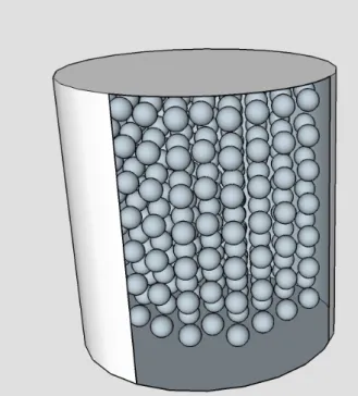
VPKT = s KKT+ 4 3µKT ρe f f , VSKT = r µKT ρe f f . (14) The Kuster-Toksöz model equations are described for a two-phase medium. Thus, the inclusion form, concentrations, matrix material and the effective elastic modulus from the proprieties can be determined (Kuster & Toksöz, 1974). The effective models of Maxwell-Garnett and of Kuster-Toksöz depend on number of inclusions, inclusion form (showed in Fig. 1) and background material of each sample, which will be described in the next section.
EXPERIMENTAL METHODOLOGY
The construction of the heterogeneous synthetic models as well as the ultrasonic measurements (P/S) was carried out at the Laboratory of Petrophysics and Rock Physics-Dr. Om Prakash Verma (LPRP), at Universidade Federal do Pará (UFPA).
Construction of samples
The synthetic model production process starts with the establishment of three groups with four samples in each one. In the groups, the samples are subdivided into types A, B, C, and a sample without heterogeneities for reference. These groups
will be subdivided by the heterogeneity quantity and also by the average diameter of the heterogeneities of each sample group, which were 4.0, 5.5 and 7.0 mm, respectively. After the definition of these factors, the next step was to determine the percentage of sieved sand and cement to satisfy the study synthetic sample, which was 30% of cement and 70% of sand in order to simulate a sandstone (with primary average porosity of 19% and density of 1.83 g/cm3). Adding a certain quantity of water to this mixture, it
gained a consistency that enabled its transference to the container.
Figure 1 – Type of samples to be constructed in this study. The shape of all samples represents a cylindrical plug with spherical heterogeneities.
Table 1 – Sample subdivision into groups A, B, and C. The numbers represent the quantity of inclusion by sample. The inclusion diameters in groups A, B, and C are 4.0, 5.5, and 7.0 mm, respectively.
Group A A-10 A-20 A-30 A-40 Group B B-10 B-20 B-30 B-40 Group C C-10 C-20 C-30 C-40
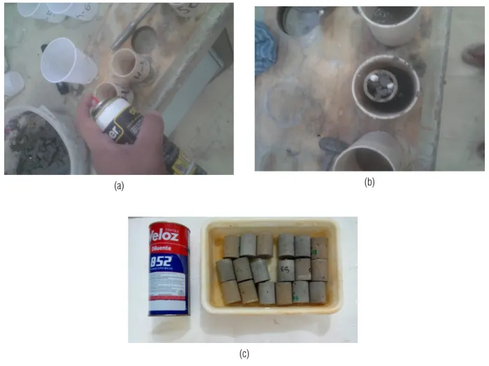
To these processes, it was used a container (tube) 60 mm high approximately with a diameter of 37.56 mm for the mixture and heterogeneities. Petroleum jelly was also used to facilitate the removal of the sample from the tube (Fig. 2a). Another 20.48 mm tube was used in the heterogeneity allocation process.
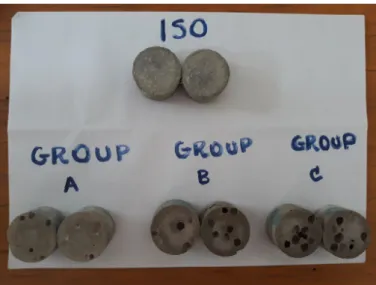
The purpose of this tube was to keep the heterogeneities well centralized, preventing them to move to the sides (Fig. 2b). Hence, the models showed in Figure 3 were made and then subdivided into three sample groups (A, B, and C) as Table 1 shows. The numbers next to the letters are the numbers of heterogeneities put in each sample.
After the mass allocation process, the sample remained 48 hours for drying at room temperature. This period provided a solidification to the sample without creating fissures. After solidification, the samples were placed in paint thinner in order to dilute all polystyrene (heterogeneities) beads to only remain empty spherical spaces (Fig. 2c). After the mass allocation process, the sample remained 48 hours for drying at room temperature. This period provided a solidification to the sample without creating fissures. After solidification, the samples were placed in a liquid in order to dilute all heterogeneities to only remain empty spherical spaces (Fig. 2c). This technique was developed by Santos et al. (2017) to create heterogeneous and anisotropic models. In order to prove this process, the samples were cut and sorted by group to acquire a good visualization of the heterogeneities (see Fig. 4).
Ultrasonic Measurements
The ultrasonic data collection was carried out using the LPFR ultrasonic system. The ultrasonic pulse transmission technique was also used (Santos et al., 2016). This system is composed by a pulse generator and receptor 5072PR and a preamplifier 5660B, both from Olympus; a 50 MHz USB oscilloscope from Handyscope; and four transducers (two 1 MHz transducers (P-wave) and two 500 kHz transducers (S-wave)), from Olympus. Figure 6 shows the experimental setup used in this work. Our transducer has an intrinsic delay time of 0.14 s (Santos et al., 2016) in its signal, which must be taken into account when estimating the wave velocities. The complete description of the ultrasonic experimental setup including the frequency source spectra is described by De Figueiredo et al. (2018) and Henriques et al. (2018). The sampling rate by channel for all measurements of the P- and S-waveforms was 0.01 s. For measurement, the transducers were sorted by the model length. Besides, they were centralized in the samples to ensure the wave propagation was in the desired region, because the heterogeneities are right in the model center. This procedure was also used for P- and S-wave acquirement.
(a) (b)
(c)
Figure 2 – (a) The petroleum jelly that is used to facilitate sample removal, (b) the use of the tube to locate the polystyrene beads so that they are centered and (c) the dissolution process in which the paint tinner is used to dissolve the styrofoam balls.
Figure 4 – Image of some cut samples that show the empty spaces (the heterogeneities) after the use of thinner for the chemical leaching.
0 10 20 30 40 50 Time [ s] -2 0 2 4 Dry : P/S wave C-10 P/S wave 0 10 20 30 40 50 Time [ s] -2 0 2 4 Dry : P/S wave C-20 0 10 20 30 40 50 Time [ s] -2 0 2 4 Dry : P/S wave C-30 0 20 40 50 Time [ s] -2 0 2 Dry : P/S wave C-40 P/S wave P/S wave P/S wave Amplitude (mV) Amplitude (mV) Amplitude (mV) Amplitude (mV)
Figure 5 – The P/S wave seismograms for group C samples in a dry condition.
RESULTS AND DISCUSSIONS
Initially the ultrasonic data obtained by the LPRP/UFPA ultrasonic system were edited and processed using the MatLab software. Due to the presence of random noise inherent to the measurement system, a data smoothing was applied to eliminate random and network noises. Figure 5 chart shows only the seismic trace for the C sample group. A manual picking of the arrival times of the P- and S-waves was carried out. Tables 2, 3 and 4 show by
group the transit times (for P- and S-waves) for each sample. The velocities of these waves can be found considering the arrival times of the seismic traces and the length and time values (Tables 2, 3 and 4). For experimental velocity estimation, errors were considered due to the measurements of length (margin of error =± 0.02 cm) and time travel picking (margin of error = ± 0.02 microseconds (µs)). The uncertainties for P- and S-wave velocity estimation ranged from ± 22.53 to ± 37.72 m/s and ± 17.07 to ± 27.48 m/s.
Figure 6 – The image of ultrasonic system used on LPRP/UFPA. Here, it is showing the Pulse-Receiver, oscilloscope and the transducers acting on a sythentic sample.
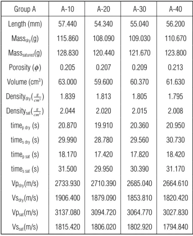
Table 2 – Sample physical parameter description for group A samples. This table shows P-and S-wave velocities for the dry P-and saturated conditions.
Group A A-10 A-20 A-30 A-40 Length (mm) 57.440 54.340 55.040 56.200 Massdry(g) 115.860 108.090 109.030 110.670 Masssatured(g) 128.830 120.440 121.670 123.800 Porosity (φ) 0.205 0.207 0.209 0.213 Volume (cm3) 63.000 59.600 60.370 61.630 Densitydry(cmg3) 1.839 1.813 1.805 1.795 Densitysat(cmg3) 2.044 2.020 2.015 2.008 timep dry(s) 20.870 19.910 20.360 20.950 times dry(s) 29.990 28.780 29.560 30.730 timep sat(s) 18.170 17.420 17.820 18.420 times sat(s) 31.500 29.950 30.390 31.170 Vpdry(m/s) 2733.930 2710.390 2685.040 2664.610 Vsdry(m/s) 1906.400 1879.090 1853.810 1820.420 Vpsat(m/s) 3137.080 3094.720 3064.770 3027.830 Vssat(m/s) 1815.420 1806.020 1802.920 1794.840
0 10 20 30 40 S ca tte ring N umbe r
2600 2800 3000 3200 V e lo c ity (m /s )
E ffective P Velocity(DRY and SA T- G roup A )- Maxwell-G arnett(MG ) and K uster-Toksöz(K T)
E xpe rime nta l S A T K T S A T MG S A T E xpe rime nta l D R Y K T D R Y MG D R Y
(a)
0 10 20 30 40
S ca tte ring N umbe r 2400 2600 2800 3000 3200 V e lo c ity (m /s )
E ffective P Velocity(DRY and SA T- G roup B )- Maxwell-G arnett(MG ) and K uster-Toksöz(K T)
E xpe rime nta l S A T K T S A T MG S A T E xpe rime nta l D R Y K T D R Y MG D R Y
(b)
0 10 20 30 40
S ca tte ring N umbe r 2400 2600 2800 3000 3200 V e lo c ity (m /s )
E ffective P Velocity(DRY and SA T- G roup C)- Maxwell-G arnett(MG) and K uster-Toksöz(K T)
E xpe rime nta l S A T K T S A T MG S A T E xpe rime nta l D R Y K T D R Y MG D R Y
(c)
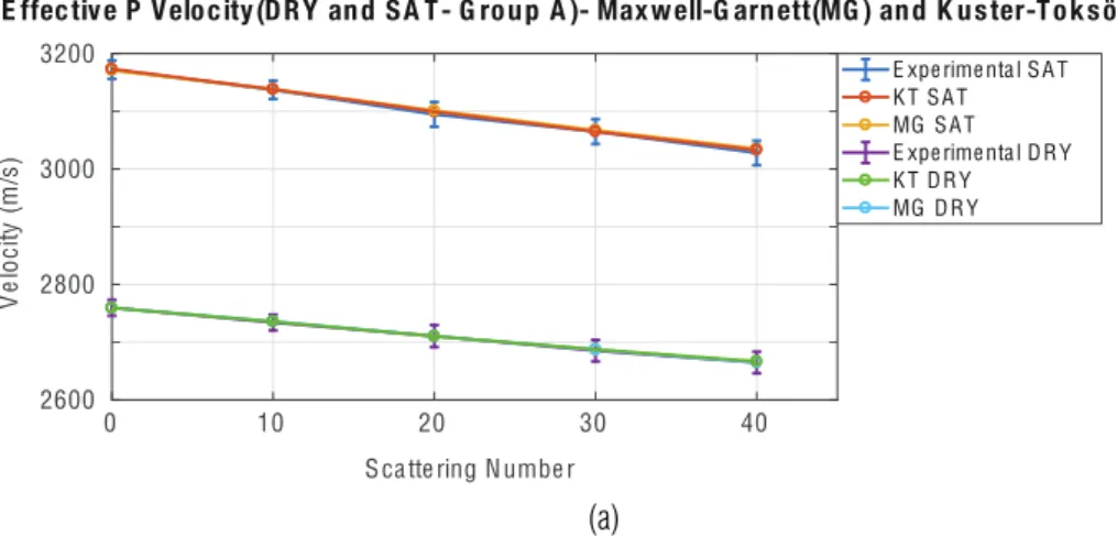
Figure 7 – The P-wave velocities as function of number of heterogeneities for different sample groups ((a) A, (b) B, and (c) C) assuming dry and saturated conditions. The purple (saturated) and blue (dry) lines show the experimental P-wave velocities.
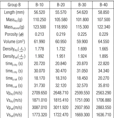
Table 3 – Sample physical parameter description for group B samples. This table shows P-and S-wave velocities for the dry P-and saturated conditions.
Group B B-10 B-20 B-30 B-40 Length (mm) 56.520 55.570 54.620 58.850 Massdry(g) 110.250 105.580 101.800 107.500 Masssatured(g) 123.500 118.950 115.300 122.340 Porosity (φ) 0.213 0.219 0.225 0.229 Volume (cm3) 61.990 60.950 59.900 64.550 Densitydry(cmg3) 1.778 1.732 1.699 1.665 Densitysat(cmg3) 1.992 1.951 1.924 1.895 timep dry(s) 20.720 20.840 20.870 22.820 times dry(s) 30.070 30.470 31.050 34.340 timep sat(s) 18.170 18.310 18.450 20.270 times sat(s) 31.730 32.120 32.570 35.810 Vpdry(m/s) 2709.650 2648.710 2599.550 2563.290 Vsdry(m/s) 1871.010 1815.410 1751.090 1706.880 Vpsat(m/s) 3087.010 3011.920 2937.950 2883.550 Vssat(m/s) 1773.320 1722.470 1669.300 1636.710
The P- and S-wave velocities (the theorethical velocities obtained from Maxwell-Garnett and Kuster-Toksöz models and the experimental velocities) in relation to the number of the heterogeneities can be observed in Figures 7 and 8. The P-wave velocities calculated for all samples present specific characteristics to each sample group: the first is the decrease of the velocity due to the increase of heterogeneities in the sample. Second, it can be observed the increase of the P velocities when the sample becomes saturated in relation to the dry case. The S velocity in this case is higher than in the saturated condition because the water does not resist to shear. Finally, the heterogeneity diameter increase results in a more pronounced decrease. Figure 7 shows the charts of the experimental and theoretical velocities in relation to the number of heterogeneities for the three sample groups. It can be noted the decrease of the P-and S-wave velocities due to the increase of scatters. It can also be noted that the heterogeneity increase affects the velocity resulting in a higher dispersion. This can be seen in the relation between groups A and C showed in 7a and 7c, respectively. Figure 7 shows that group A has a low dispersion due to the smaller heterogeneity diameters in relation to the group C diameters. Considering the dry and saturated cases, the P velocity is higher in the saturated
case than in the dry case because the saturation changes the physical proprieties turning the rock more rigid and dense. This relation can be seen in the Equations 8 and 14 of the effective models.
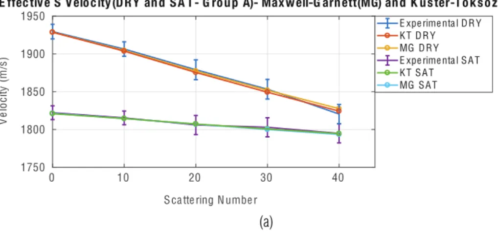
Figure 8 shows the S-wave velocity in relation to the number of heterogeneities. It can be seen the S-wave dispersion in relation to the increase of the number of scatters. It is also noted the heterogeneity diameter increase resulting in a more pronounced decrease of the velocity in relation to the groups. Another important characteristic that can be noted occurs in the dry and saturated cases. As the water does not support shear, a S-wave characteristic, the velocity in the saturated case is lower than it is in the dry case. This is also affected individually. As group A, showed in Figure 8a, presents a low scatter diameter, the water saturation in this sample group is much lower. Therefore it can be noted that the S velocity decrease of group A is lower because this sample group presents heterogeneities with a smaller diameter.
Although it is not showed here, the P- and S-wave velocities also decrease with the sample porosity increase (primary and inclusion porosity). Similar to the decrease of the scatter number, the velocities most dependent on the porosity increase were the
0 10 20 30 40 S ca tte ring N umbe r
1750 1800 1850 1900 1950 V e lo c ity (m /s )
E ffective S Velocity(DRY and SA T- G roup A)- Maxwell-G arnett(MG) and K uster-Toksöz(K T)
E xpe rime nta l D R Y K T D R Y MG D R Y E xpe rime nta l S A T K T S A T MG S A T
(a)
0 10 20 30 40
S ca tte ting N umbe r 1600 1700 1800 1900 2000 V e lo c ity (m /s )
E ffective S Velocity(DRY and SA T- G roup B)- Maxwell-G arnett(MG) and K uster-Toksöz(K T)
E xpe rime nta l D R Y K T D R Y MG D R Y E xpe rime nta l S A T K T S A T MG S A T
(b)
0 10 20 30 40
S ca tte ting N umbe r 1400 1500 1600 1700 1800 1900 2000 V e lo c ity (m /s )
E ffective S Velocity(DRY and SA T- G roup C )- Maxwell-G arnett(MG ) and K uster-Toksöz(K T)
E xpe rime nta l D R Y K T D R Y MG D R Y E xpe rime nta l S A T K T S A T MG S A T
(c)
Figure 8 – The S-wave velocities as function of number of heterogeneities for different sample groups ((a) A, (b) B, and (c) C) assuming dry and saturated conditions. The purple (saturated) and blue (dry) lines show the experimental S-wave velocities. The other curves correspond to the theoretical values obtained from Maxwell-Garnett and Kuster-Toksöz models.
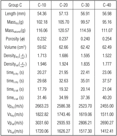
Table 4 – Sample physical parameter description for group C samples. This table shows P-and S-wave velocities for the dry P-and saturated conditions.
Group C C-10 C-20 C-30 C-40 Length (mm) 54.36 57.13 56.91 56.98 Massdry(g) 102.18 105.70 99.57 95.16 Masssatured(g) 116.06 120.57 114.59 111.07 Porosity (φ) 0.232 0.237 0.240 0.254 Volume (cm3) 59.62 62.66 62.42 62.49 Densitydry(cmg3) 1.713 1.686 1.595 1.522 Densitysat(cmg3) 1.946 1.924 1.835 1.777 timep dry(s) 20.27 21.95 22.41 23.06 times dry(s) 29.68 32.63 35.01 37.57 timep sat(s) 17.79 19.32 20.14 21.04 times sat(s) 31.46 34.99 37.36 40.20 Vpdry(m/s) 2663.23 2586.38 2523.70 2455.00 Vsdry(m/s) 1822.82 1743.46 1619.06 1511.00 Vpsat(m/s) 3031.60 2935.93 2806.21 2690.27 Vssat(m/s) 1720.06 1626.27 1517.30 1412.41
velocities that had inclusions with a larger diameter (samples of groups B and C). Experimentally, this velocity decrease related to the porosity increase was also observed by Han et al. (1986) and Castagna et al. (1986). In these studies that relate the ultrasonic wave velocities with porosity (represented by empirical models) it was observed the velocity decrease with porosity increase in siliciclastic rocks present in most of the hydrocarbon reservoirs (conventional and non-conventional).
CONCLUSIONS AND DISCUSSIONS
We tested our experimental results against predictions of effective medium models insufficiently investigated (Maxwell-Garnett and Kuster-Toksöz) from an experimental point of view. In general, for the three sample groups analyzed in this work, the P and S velocities (theoretical and experimental) decrease with the increase of the inclusion density (inclusion porosity or number of heterogeneities). This decrease (dispersion) was more prominent for the sample group with an effective diameter of 7.0 mm approximately.
It is important to mention how well the predictions of the model perform for different ranges of heterogeneity density (or porosity). Based on our results, we can conclude that even when applying the modified Maxwell-Garnett model we achieved a good agreement between the experimental results and the model predictions for a heterogeneity density interval inferior to 8%. Obviously, as expected, the prediction performed by the Kuster-Toksöz model also showed a good agreement. However, the simple mathematical formalism of Maxwell-Garnett’s model can provide its most recurrent use.
The methodology proposed here to construct synthetic heterogeneous samples proved to be quite advantageous. Our tests were very successful, proving that the dissolved styrofoam holders generate empty spherical spaces inside the samples. These samples that use low cost conventional materials (water, clay, sand, cement, calcareous, etc.) can be efficiently used to build synthetic carbonate rocks which can represent an even more valuable application of this method for hydrocarbon exploration on non-conventional reservoir. Furthermore, we suggest the
use of other effective models in order to investigate synthetic carbonate rocks.
ACKNOWLEDGMENTS
The authors would like to thank the Brazilian agencies PET/GEOFÍSICA-UFPA-Ministério da Educação, INCT-GP and CNPq (grant no. CNPq 459063/2014-6 and grant no. CNPq 140174/2016-8) from Brazil and the Geophysics Graduate Program at the Universidade Federal do Pará for the financial support in this research. The authors would also like to thank the reviewers for many helpful comments and suggestions.
REFERENCES
AHRENS TJ. 1995. Rock Physics and Phase Relations: A Handbook of Physical Constants. Washington, DC: American Geophysical Union. 384 pp.
BARWIS JH, McPHERSON JG & STUDLICK JRJ. 1990. Sandstone Petroleum Reservoirs. Spring Verlag. 583 pp.
BROWN R & KORRINGA J. 1975. On the dependence of the elastic properties of a porous rock on the compressibility of the pore fluid. Geophysics, 40(4): 608–616. doi: 10.1190/1.1440551. URL https:// library.seg.org/doi/10.1190/1.1440551.
BRUGGEMAN DAG. 1935. Erechnung Verschiedener Physikalischer Konstanten von Heterogenen Substanzen. I. Dielektrizitatskonstanten und Leitfahigkeiten der Mischkorper aus Isotropen Substanzen. Ann. Phys. (Leipzig), 24: 636–679.
CASTAGNA JP, BATZLE ML & EASTWOOD RL. 1986. Relationships between compressional wave and shear-wave velocities in clastic silicate rocks. Geophysics, 50(4): 571–581.
DE FIGUEIREDO JJS, DO NASCIMENTO MJS, HARTMANN E, CHIBA BF, DA SILVA CB, DE SOUSA MC, SILVA C & SANTOS LK. 2018. On the application of the Eshelby-Cheng effective model in a porous cracked medium with background anisotropy: An experimental approach. Geophysics, 83(5): C209–C220.
HAN DH, NUR A & MORGAN D. 1986. Effects of porosity and clay content on wave velocities in sandstones. Geophysics, 51(11): 2093–2107. HENRIQUES JP, DE FIGUEIREDO JJS, SANTOS LK, MACEDO DL, COUTINHO I, DA SILVA CB, MELO LA, SOUSA M & AZEVEDO FL. 2018. Experimental verification of effective anisotropic crack theories in variable crack aspect ratio medium. Geophysical Prospecting, 66(11): 141–156.
KUSTER G & TOKSÖZ M. 1974. Velocity and attenuation of seismic waves in two-phase media: part I. theoretical formulations. Geophysics, 39(5): 587–606. doi: 10.1190/1.1440450. URL https://library.seg.org/ doi/10.1190/1.1440450.
MARKEL VA. 2016. Introduction to the Maxwell Garnett approximation: tutorial. Journal of the Optical Society of America A, 33: 1244–1256. MAVKO G, MUKERJI T & DVORKIN J. 2009. The Rock
Physics Handbook. Cambridge University Press. doi:
10.1017/CBO9780511626753. 524 pp.
MAXWELL-GARNETT JC. 1904. Colours in Metal Glasses and Metal Films. Philos. Trans. R. Soc. London Ser. A, 203: 385–420.
SANTOS LK, DE FIGUEIREDO JJS & DA SILVA CB. 2016. A study of ultrasonic physical modeling of isotropic media based on dynamic similitude. Ultrasonics, 70: 227–237.
SANTOS LK, DE FIGUEIREDO JJS, MACEDO DL & DA SILVA CB. 2017. A new way to construct synthetic porous fractured medium. Journal of Petroleum Science and Engineering, 156: 763–768.
Recebido em 22 setembro, 2018 / Aceito em 30 novembro, 2018 Received on September 22, 2018 / accepted on November 30, 2018