ANALYSIS OF WELL-BEING IN OECD COUNTRIES THROUGH STATIS METHODOLOGY

(1)

HOLOS, Year 32, Vol. 7 335

ANALYSIS OF WELL-BEING IN OECD COUNTRIES THROUGH STATIS METHODOLOGY

F. J. RIVADENEIRA1*_{, A. M. S. FIGUEIREDO}2_{, F. O. S. FIGUEIREDO}3_{, S. M. CARVAJAL}4_{and R. A. RIVADENEIRA}5

1_{Facultad de Ciencias Informáticas, Universidad Laica Eloy Alfaro de Manabí – ULEAM}

2_{Faculdade de Economia, Universidade do Porto and INESC – TEC Porto}

3_{Faculdade de Economia, Universidade do Porto and CEAUL}

4_{Facultad de Economía, Universidad Técnica de Manabí – UTM}

5_{Facultad de Ingeniería Química, Universidad Técnica de Manabí – UTM}

fabricio.rivadeneira@uleam.edu.ec*

Article received in August/2016 and accepted in October/2016 DOI: 10.15628/holos.2016.5003

ABSTRACT

This paper presents the main concepts and results of a Master thesis in Data Analysis which aims to analyze the evolution of some developed countries and also of some emerging countries that are members of the Organisation for Economic Co-operation and Development (OECD) in what concerns some indicators or variables of well-being during the period 2011-2015, through the STATIS (Structuring Three-way data sets in

Statistics) methodology. This methodology allows to analyze the presence of a common structure in several data tables obtained over time, to identify the differences and similarities along the period of time under study and according to well-being indicators included in the “Your Better Life Index” of the OECD, and to analyze the trajectories of the countries.

KEYWORDS: Principal Component Analysis, STATIS methodology, Three-way data methods, well-being indicators.

ANÁLISIS DE BIENESTAR EN LOS PAÍSES DE LA OCDE A TRAVÉS DE LA

METODOLOGÍA STATIS

RESUMO

Este artículo presenta los conceptos y resultados principales de una tesis de Maestría en Análisis de Datos que tiene como objetivo analizar la evolución de algunos países desarrollados y también de algunos países emergentes que son miembros de la Organización para la Cooperación y el Desarrollo Económicos (OCDE) en lo que se refiere a algunos indicadores o variables de bienestar durante el período 2011-2015, a través de la

metodología STATIS (Estructura Estadística de una Tabla de Tres Índices). Esta metodología permite analizar la presencia de una estructura común en varias tablas de datos obtenidos a lo largo del tiempo, para identificar las diferencias y similitudes a lo largo del periodo de tiempo en estudio y de acuerdo con los indicadores de bienestar incluido en el “Índice para una Vida Mejor” de la OCDE, y para analizar las trayectorias de los países.

PALAVRAS-CHAVE: Análisis de Componentes Principales, metodología STATIS, métodos de datos de tres índices,

(2)

1 INTRODUCTION

Currently there are a special interest in the joint analysis of multiple data tables, named several multi-blocks or multi-way analysis. Most of these methods are extensions of Principal Component Analysis. On the other hand, there is also a global interest in analyzing the well-being and the progress of countries, like the Better Life Index created by the Organisation for Economic Co-operation and Development (OECD, 2016) and the Social Progress Index created by Social Progress Imperative organization (Social Progress Imperative, 2016).

Thus, the methodology chosen in this paper is STATIS (‘Structuration des Tableaux À Trois Indices de la Statistique’ in French or ‘Structuring Three-way data sets in Statistics’ in English), that is one of the methods for developing other complex techniques of joint analysis of several data sets, and it is applied in the analysis of OECD countries using well-being indicators.

The statistical databases online platform of the OECD (2015) includes data tables for analyzing the well-being of societies, each table contains between 17 and 24 indicators or quantitative variables, and it depends of the availability of the countries in gathering the information. These indicators focus on eleven aspects or dimensions of life that matter to people, and represent key factors, like housing, income, jobs, community, education, environment, civic engagement, health, life satisfaction, safety, work-life balance (OECD, 2013). So, these eleven dimensions of the index are currently based on one to four indicators. All these data from OECD can be presented in a multi-block data structure.

Since OECD data of countries are essentially multi-block data tables, multi-block component methods can be used for analyzing differences or similarities between OECD tables. Through the joint analysis of multiple data tables using the STATIS methodology, this paper proposes to analyze a set of tables used to calculate the Better Life Index in OECD countries, in order to know the performance of 34 member countries, as well as their trends in the 2011-2015 period. For that, we used several tables, where each table contains a set of well-being indicators of the OECD countries for a specific year.

Thereby, the main objective of this paper is to obtain a structure common of the data tables that best represents the differences and similarities among the years according to the performances of the OECD countries related to the well-being indicators. This aims to summarize the information contained in the various data tables and additionally, to analyze trends representing the trajectories of the countries through the years, identifying and explaining what countries are responsible for the differences detected between the various data tables.

1.1 Research questions

So, several data tables from OECD countries are considered corresponding to different

years, thus this study was shaped by the following research questions:

• How to handle with various data tables that measure sets of well-being indicators

(3)

• How to analyze several data tables that have been collected in different moments of time to determine a common structure associated to the OECD countries that best represents similitudes between the different data tables?

• How to compare globally the several data tables and which countries are responsible for the differences detected between the several data tables?

2 STATE-OF-THE-ART

2.1 Some basic definitions

According to the particular structure of data, the data sets take different names, Rivadeneira (2016) shows some common structures and names.

2.1.1 Multi-Block data tables

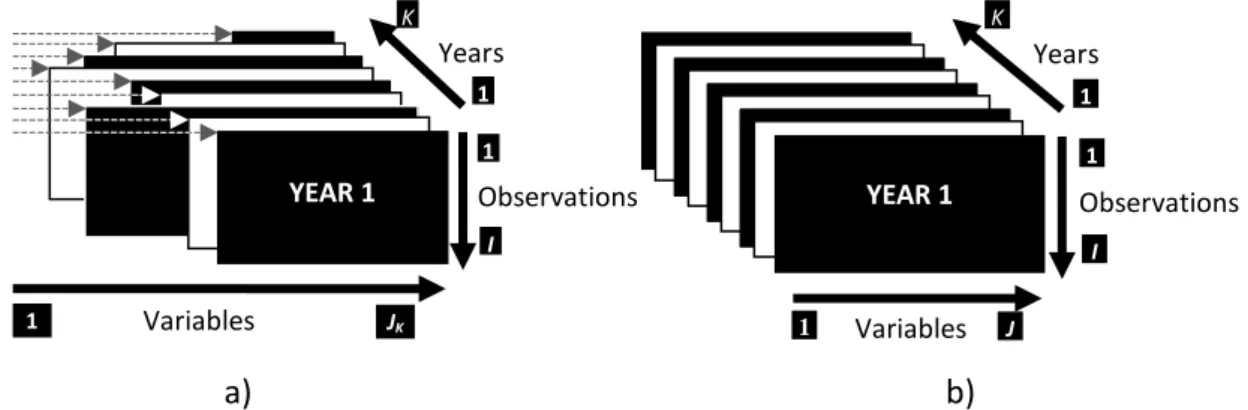
Several data tables that have a common dimension between them, i.e. either the same rows or the same columns, but not necessarily both. Each group of variables, or each matrix, is usually called a block or a configuration and in general is measured on the same observations, as shown in Figure 1a.

a) b)

Figure 1: General structure of data - a) multi-block data or multiple tables; b) three-way data sets or third order tensor.

In Figure 1a, for each year (k), there is a data table consisting of measurements for a

number of JK attributes, but the number of JK attributes can vary for each year, and the number

of I observations remains the same.

2.1.2 Three-way data tables

There are data tables that can be presented in a three way, three mode or third dimension data structure as shown in Figure 1b, for each year (k), there is a data table consisting of measurements for a number of J attributes and a number of I observations. In most of the cases, multiway data tables contain the same number of rows and same number of columns

2.2 Overview of joint Analysis methods of tables

It is important to consider the different structures of data in order to decide the specific method of data analysis that must be applied such as multi-block methods, three-way analysis

Years YEAR 1 Observations 1 I 1 K Variables 1 JK Years YEAR 1 _Observations 1 I 1 Variables 1 J K

(4)

methods, methods on instrumental variables, multiway analysis, and so on. Then, there are a lot of possible methods that researchers can consider for the analysis of multiple data tables, Rivadeneira (2016) divided in two categories: analysis of multiple tables or multi-block and three-way data tables, and methods for two or more multi-blocks data and multi-three-way data, as shown in Table 1.

There is other classification about the overview of analysis methods for multi-group data in Eslami et al. (2013).

Table 1: Methods for the analysis of multiple data tables.

Data Structure Method or Technique Reference

Multiblock or three-way data

STATIS: Structuring Three-way data sets in Statistics, and Dual STATIS.

CCSWA: Common Components and Specific Weights Analysis, and Dual CCSWA.

MUDICA: Multiblock Discriminant Correspondence Analysis. DACP: Double Principal Component Analysis.

Multi-Block PCA or Multi-Groups PCA.

MFA: Multiple Factor Analysis, also called Multiple Factorial Analysis, and Dual-MFA.

GPA: Generalized Procruste Analysis, and Dual GPA.

(Lavit et al., 1994) (Qannari et al., 2001) (Abdi et al., 2010) (Bouroche, 1975) (Derks et al., 2003) (Escofier & Pagés, 1994) (Gower, 1975)

Several multi-blocks

or multi-way data

GOMCIA: Generalized Orthogonal Multiple Co-Inertia Analysis. DO-ACT: DOuble-Analyse Conjointe de Tableaux, or Double-STATIS is a generalization of Double-STATIS.

HMFA: Hierarchical Multiple Factor Analysis.

MMCovC: Multiway Multiblock Covariate Component.

PARAFAC: Parallel Factor Analysis, and PARAFAC-family and derivatives models.

Tucker, and Tucker-family and derivatives models. Tensor Data Analysis.

STATIS-4 an extension of STATIS and DO-ACT.

(Vivien & Sune, 2009) (Vivien & Sune, 2009) (Le Dien & Pagés, 2003) (Smilde, 2000)

(Acar & Yener, 2009) (Acar & Yener, 2009) (Kolda & Bader, 2009) (Sabatier & Vivien, 2008)

2.3 Related works about STATIS

Based only on STATIS methodology as a common framework, some methods of joint analysis of tables have been developed, like DO-ACT, STATIS-4 and others (Abdi et al., 2012).

Also there are some applications of this method in several areas, for example: Gonçalves (2010) studied the performance or evolution of economic activities in Portugal analyzing the information obtained along the years by Bank of Portugal and identifying differences and similarities between years and trends over time for those activities; Brás (2012) uses the information provided by the National Statistical Institute of Portugal (INE) and analyzed the evolution of the construction sector in Portugal in order to offer a better understanding of the Portuguese construction sector over the time; Lourenço (2013) analyzed the vulnerability indicators present in the Early Warning Systems (EWS) of European countries, detecting the main economic weaknesses that contributes to predict the occurrence of a crisis in a certain time horizon; Stanimirova et al. (2004) applied STATIS for the exploration of three-way environmental data, and compares its performance with Tucker3 and PARAFAC2 methods; González et al. (2005)

(5)

analyzed the consumption of electrical power in a hotel during the months that the environmental conditions differ the most, to determine the appropriate actions on the way to its saving; Chaya et al. (2004) applied this methodology for the analysis of time-intensity profiling data, with sensory attributes of ranch salad dressing as variables, and a set of products as objects; Amendola et al. (2006) studied the causes of the socio-economic disparities among the European regions; Figueiredo et al. (2012) analyzed the dynamics and evolution of the structural economic reforms during the period 1989 –1996 where the privatization of state-owned enterprises taking place in the Portuguese banking sector.

Almeida (2012) applied a variant of this methodology called Dual STATIS in a data set that records information about cycles of couples with infertility diagnosis of the Assisted Medical Reproduction Center in Oporto Hospital to understand which variables contribute the most to the differences between the groups of couples. The method allowed us to discover a greater proximity between groups composed of couples who are not pregnant and a greater distance between the groups of couples who become pregnant. Also, Coquet et al. (1996) adapted STATIS, obtaining significant acceleration to study and characterize the internal molecular motions and conformations from a large number of molecular dynamics sets of coordinates, when simulated in a solution by molecular dynamics techniques.

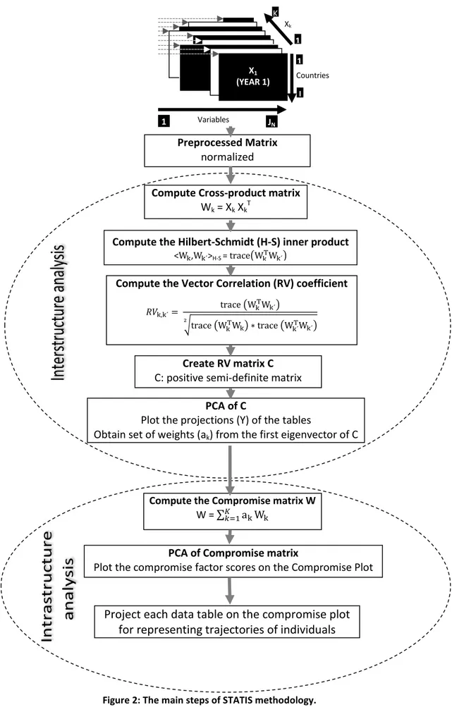
3 METHODOLOGY

The STATIS methodology was firstly developed in the Statistics and Probability Laboratory of the University of Montpellier II by Escoufier (1973) and his team and by L’Hermier des Plantes (1976) and later developed by Lavit (1988) and Lavit et al. (1994). It lets you extract information from multidimensional data collected in diverse situations or time instants.

The STATIS methodology requires that the observations, countries in our case, must be the same for all data tables, and can be seen as an extension of Principal Component Analysis for the analysis of multiple data tables that measure sets of variables collected on the same observations. STATIS does not require the data tables to have the same number of columns. A sketch of all these steps is provided in Figure 2.

The 5 data tables used for measuring the well-being of societies came from 2011 to 2015 with the same countries described by seventeen to twenty-four quantitative variables, are formed as follows:

• The data table from 2011 has 34 countries presented in rows and 17 indicators presented in columns.

• The data tables from 2012 to 2015 have 34 countries presented in rows and 24 indicators presented in columns, for each table.

This work was developed using the software of data analysis SPAD version 8.0, R language and Excel for the implementation of the Statis methodology.

(6)

Figure 2: The main steps of STATIS methodology.

Xk X1 (YEAR 1) Countries 1 I 1 K Variables 1 JN Preprocessed Matrix normalized

Compute Cross-product matrix

Wk = Xk XkT

Compute the Hilbert-Schmidt (H-S) inner product

<Wk,Wk´>H-S = trace�W_kTWk´� 𝑅𝑅k,k´= trace �Wk T_W k´� �trace �WkTWk� ∗ trace �Wk´TWk´� 2

Compute the Vector Correlation (RV) coefficient

Create RV matrix C

C: positive semi-definite matrix

PCA of C

Plot the projections (Y) of the tables

Obtain set of weights (ak) from the first eigenvector of C

Compute the Compromise matrix W

W = ∑𝐾𝑘=1akWk PCA of Compromise matrix

Plot the compromise factor scores on the Compromise Plot

Project each data table on the compromise plot for representing trajectories of individuals

(7)

4 RESULTS AND DISCUSSIONS

The results are presented following the STATIS methodology allowing the analysis of a possible common structure for the data tables that best represents the similarities among the years and, the evolution of the OECD countries described by the indicators considered in the study. The data were centered and reduced because the variables are heterogeneous, with different units.

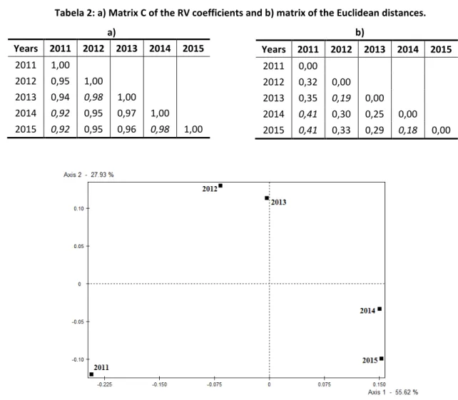
4.1 Interstructure

The first phase of the Statis method compute the cross-product matrix between countries for each data table with their indicators of well-being as a representative object of each table, corresponding to each year under study. Then, a global comparison between data tables is done using the RV coefficient, in which we conclude what years are more similar and what are more different.

So, through the analysis of the Tables 2a and 2b about the RV coefficients and the Euclidean distances, respectively, we can conclude that the years 2012 and 2013, 2014 and 2015 are the closest, with a RV coefficient of 0,98, and a distance between these years of 0,19 and 0,18 respectively; while the pairs of years 2011 and 2014, 2011 and 2015 are the most different, with a RV coefficient of 0,92, and a distance between these years of 0,41.

Tabela 2: a) Matrix C of the RV coefficients and b) matrix of the Euclidean distances. a) b) Years 2011 2012 2013 2014 2015 2011 1,00 2012 0,95 1,00 2013 0,94 0,98 1,00 2014 0,92 0,95 0,97 1,00 2015 0,92 0,95 0,96 0,98 1,00

Figure 3: Centred interstructure Euclidean image.

Years 2011 2012 2013 2014 2015 2011 0,00 2012 0,32 0,00 2013 0,35 0,19 0,00 2014 0,41 0,30 0,25 0,00 2015 0,41 0,33 0,29 0,18 0,00

(8)

By diagonalization of the matrix of RV coefficients, we obtain a system of axes associated to the eigenvalues as well as the percentage of inertia explained by each axis, then in the plan defined by the first and second axes we can see in the Figure 3 the short distance between the years 2012 and 2013, 2014 and 2015 which indicates proximity or similarity between these years, while the years 2011 and 2014, 2011 and 2015 are more distant between them, and which show the same results we had from Table 2a and 2b.

4.2 Intrastructure

In this step, we compute the compromise matrix defined as a linear combination of the objects, weighted by the coordinates of the objects on the first axis of the Interstructure. Table 3 contains the scalar products or correlations between normed objects and the Euclidean distances between objects and the compromise, indicating the years closest and the most distant in relation to the compromise.

Thus, through the analysis of the scalar products and the Euclidean distances, we can conclude that the years are highly correlated with the compromise, because in general distances are low and scalar products are high, proving that it is possible to find a common structure; being the year of 2013 the one that has the highest correlation with the compromise, and the year of 2011 the one with the smallest correlation.

Table 3: Scalar products and distances to the compromise object

2011 2012 2013 2014 2015

Scalar Products 0,963 0,985 0,989 0,984 0,980

Euclidean Distances 0,272 0,171 0,148 0,180 0,199

Applying PCA to the compromise object, we considered the first five axes because the first five axes explain 70,97% of the total inertia. Therefore, the following figures: Figures 4, 5, 6 and 8 are the graphical representations for the five axes, which show the countries’ compromise Euclidean image in the plan defined by the first and second axes [1, 2], the first and third axes [1, 3], the first and fourth axes [1, 4], and in the plan defined by the first and fifth axes [1, 5], respectively.

In these figures, the farthest countries from the center are the countries that most contribute to the formation of the axis and are selected so that the sum of their contributions to the axis is about 80%. Additionally, all the countries selected for the axis have a contribution greater than the average contribution of a country and are well represented on that axis. The coordinates, absolute and relative contributions of the countries in the first five axes were taken into account for the interpretation of the axes, and for the interpretation of the compromise axes, we determined the linear correlations between the initial variables and the compromise axes.

Figure 4 shows that the countries with the greatest importance on the first axis are Switzerland (che), Canada (can), Turkey (tur), Mexico (mex) and Chile (chl). So, the first axis makes a distinction between Turkey, Mexico and Chile (all with negative coordinates) and the countries Switzerland and Canada (with positive coordinates).

The first axis is positively correlated with the variable Rooms per person (RmPS), Household net adjusted disposable income (HDIn), Employment rate (Empl), Personal earnings

(9)

(Pear), Quality of support network (QSNw), Water quality (WatQ), Life expectancy (LfEx) and negatively correlated with Dwellings without basic facilities (DwoF), during all period. Therefore, the first axis opposes Switzerland and Canada with high values in variables RmPS, HDIn, Empl, PEar, QSNw, WatQ, LfEx and low value in Dwellings without basic facilities to Turkey, Mexico and Chile with low values in the variables RmPS, HDIn, Empl, PEar, QSNw, WatQ, LfEx and high value in DwoF.

Figure 4: Countries’ compromise Euclidean image in the plan [1, 2].

The fourth axis (see Figure 6) opposes Mexico (mex) with negative coordinate to the countries with positive coordinates, like Korea and Japan. The fourth axis is negatively correlated with the variable Homicide rate (Homd), during all period. So, the fourth axis apposes Mexico to Korea and Japan because the Mexico with negative coordinate have high values in Homicide rate (Homd), while the countries Korea and Japan with positive coordinates have low values in Homd.

(10)

Finally, the variable that is more correlated with the fifth axis is Consultation on rule-making (CoRl) and it is positively correlated, so from Figure 7, this axis opposes the countries Chile (chl), Israel (isr) and Japan (jpn) (positive coordinates) with high values in CoRl to the countries New Zealand (nzl), Australia (aus) (negative coordinates) with low values in the variable CoRl.

Figure 7: Countries’ compromise Euclidean image in the plan [1, 5]. 4.3 Trajectories

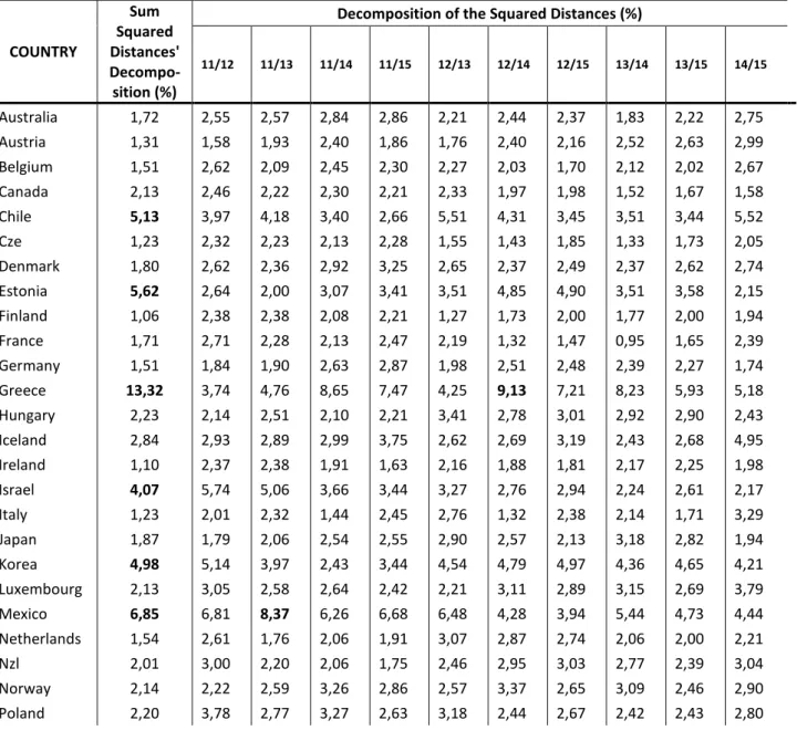
In this step it is important to highlight the countries that are responsible for the differences between the various years. Table 4 shows the decomposition of the sum of squared distances between normed objects into percentage of countries’ contributions allows to identify which countries have contributed more to the differences during all the period 2011 - 2015: Greece (13,32%), Turkey (7,30%), Mexico (6,85%), Spain (6,22%), Estonia (5,62%), Chile (5,13%), Korea (4,98%), Israel (4,07%), and Slovak Republic (3,57%). The countries that less contribute are Finland (1,06%), Ireland (1,10%) and Sweden (1,18%).

The decomposition of the squared distances between pairs of normed objects, Table 4, allows to stand out which countries have contributed more for the differences between couple of years. Greece is responsible for these differences for any couple of years here considered, with the highest contribution between 2012 and 2014 (9,13%) and less significant between 2011 and 2012 (3,74%). Another countries that also generally contribute to the structural differences are Turkey and Mexico, in particular, between 2011 and 2013 (8,67% and 8,37% respectively).

(11)

Figure 8 shows the trajectories in the plan [1, 2] that explains 50.18% of the total variance. Although the representation of the trajectories is approximated, their irregularities are visibly presented.

The first axis is positively correlated with the variable Rooms per person, Household net adjusted disposable income, Employment rate, Personal earnings, Quality of support network, Water quality and Life expectancy and negatively correlated with Dwellings without basic facilities. Thus, as the trajectory evolution of Estonia, Germany and Iceland is from the left to the right side, it can indicate progress in the OECD well-being conceptual dimensions, in contrast to Greece, Israel and Mexico, whose trajectory evolution is from the right to left side. Hungary and Korea have a more elongated down to up trajectory in relation to the second axis, which can indicate a reduction of unemployed for one year or more, as the second axis is negatively correlated with the variable Long-term unemployment rate, differentiating countries like, Greece and Spain.

Table 4: Scalar products and distances to the compromise object

COUNTRY Sum Squared Distances' Decompo-sition (%)

Decomposition of the Squared Distances (%)

11/12 11/13 11/14 11/15 12/13 12/14 12/15 13/14 13/15 14/15 Australia 1,72 2,55 2,57 2,84 2,86 2,21 2,44 2,37 1,83 2,22 2,75 Austria 1,31 1,58 1,93 2,40 1,86 1,76 2,40 2,16 2,52 2,63 2,99 Belgium 1,51 2,62 2,09 2,45 2,30 2,27 2,03 1,70 2,12 2,02 2,67 Canada 2,13 2,46 2,22 2,30 2,21 2,33 1,97 1,98 1,52 1,67 1,58 Chile 5,13 3,97 4,18 3,40 2,66 5,51 4,31 3,45 3,51 3,44 5,52 Cze 1,23 2,32 2,23 2,13 2,28 1,55 1,43 1,85 1,33 1,73 2,05 Denmark 1,80 2,62 2,36 2,92 3,25 2,65 2,37 2,49 2,37 2,62 2,74 Estonia 5,62 2,64 2,00 3,07 3,41 3,51 4,85 4,90 3,51 3,58 2,15 Finland 1,06 2,38 2,38 2,08 2,21 1,27 1,73 2,00 1,77 2,00 1,94 France 1,71 2,71 2,28 2,13 2,47 2,19 1,32 1,47 0,95 1,65 2,39 Germany 1,51 1,84 1,90 2,63 2,87 1,98 2,51 2,48 2,39 2,27 1,74 Greece 13,32 3,74 4,76 8,65 7,47 4,25 9,13 7,21 8,23 5,93 5,18 Hungary 2,23 2,14 2,51 2,10 2,21 3,41 2,78 3,01 2,92 2,90 2,43 Iceland 2,84 2,93 2,89 2,99 3,75 2,62 2,69 3,19 2,43 2,68 4,95 Ireland 1,10 2,37 2,38 1,91 1,63 2,16 1,88 1,81 2,17 2,25 1,98 Israel 4,07 5,74 5,06 3,66 3,44 3,27 2,76 2,94 2,24 2,61 2,17 Italy 1,23 2,01 2,32 1,44 2,45 2,76 1,32 2,38 2,14 1,71 3,29 Japan 1,87 1,79 2,06 2,54 2,55 2,90 2,57 2,13 3,18 2,82 1,94 Korea 4,98 5,14 3,97 2,43 3,44 4,54 4,79 4,97 4,36 4,65 4,21 Luxembourg 2,13 3,05 2,58 2,64 2,42 2,21 3,11 2,89 3,15 2,69 3,79 Mexico 6,85 6,81 8,37 6,26 6,68 6,48 4,28 3,94 5,44 4,73 4,44 Netherlands 1,54 2,61 1,76 2,06 1,91 3,07 2,87 2,74 2,06 2,00 2,21 Nzl 2,01 3,00 2,20 2,06 1,75 2,46 2,95 3,03 2,77 2,39 3,04 Norway 2,14 2,22 2,59 3,26 2,86 2,57 3,37 2,65 3,09 2,46 2,90 Poland 2,20 3,78 2,77 3,27 2,63 3,18 2,44 2,67 2,42 2,43 2,80

(12)

HOLOS, Year 32, Vol. 7 346 Portugal 1,96 1,70 1,59 2,04 2,05 2,03 2,59 2,57 2,47 2,50 3,00 Svk 3,57 2,62 3,04 3,07 3,18 2,83 2,99 3,11 2,50 2,72 2,38 Slovenia 1,32 2,20 2,10 1,88 2,05 2,01 1,44 1,49 1,50 2,18 3,22 Spain 6,22 1,44 1,22 4,61 4,97 2,82 6,06 5,93 6,67 6,23 2,70 Sweden 1,18 2,18 2,37 1,91 2,11 2,14 1,75 1,92 1,89 1,97 2,33 Switzerland 2,17 3,17 3,50 3,31 3,39 2,39 2,47 2,83 2,74 2,96 2,90 Turkey 7,30 6,22 8,67 5,06 4,08 7,85 4,53 4,95 7,47 7,80 4,47 Gbr 1,59 2,90 3,04 2,28 1,88 2,00 1,54 2,24 2,52 3,35 2,67 USA 1,44 2,55 2,10 2,24 2,73 2,81 2,34 2,54 1,82 2,21 2,48

(13)

Figure 7: Countries’ trajectories in the plan [1, 2]

[CELLRANGE] [CELLRANGE] [CELLRANGE] [CELLRANGE] [CELLRANGE] 0,000 0,020 0,040 0,060 -0,003 0,007 0,017 0,027 0,037 0,047 2nd A xi s 1st Axis Austria [CELLRANGE] [CELLRANGE] [CELLRANGE] [CELLRANGE] [CELLRANGE] 0,000 0,020 0,040 0,060 0,035 0,045 0,055 0,065 0,075 0,085 2nd A xi s 1st Axis Australia [CELLRANGE] [CELLRANGE] [CELLRANGE] [CELLRANGE] [CELLRANGE] 0,000 0,020 0,040 0,060 -0,003 0,007 0,017 0,027 0,037 0,047 2nd A xi s 1st Axis Belgium [CELLRANGE] [CELLRANGE] [CELLRANGE] [CELLRANGE] [CELLRANGE] 0,000 0,020 0,040 0,060 -0,170 -0,160 -0,150 -0,140 -0,130 -0,120 2nd A xi s 1st Axis Chile [CELLRANGE] [CELLRANGE] [CELLRANGE] [CELLRANGE] [CELLRANGE] 0,000 0,020 0,040 0,060 0,058 0,068 0,078 0,088 0,098 0,108 2nd A xi s 1st Axis Canada [CELLRANGE] [CELLRANGE] [CELLRANGE] [CELLRANGE] [CELLRANGE]

-0,070 -0,050 -0,030 -0,010 -0,035 -0,025 -0,015 -0,005 0,005 0,015 2nd A xi s 1st Axis Czech Republic [CELLRANGE] [CELLRANGE] [CELLRANGE] [CELLRANGE] [CELLRANGE] -0,080 -0,060 -0,040 -0,020 -0,120 -0,110 -0,100 -0,090 -0,080 -0,070 2nd A xi s 1st Axis Estonia [CELLRANGE] [CELLRANGE] [CELLRANGE] [CELLRANGE] [CELLRANGE] -0,070 -0,050 -0,030 -0,010 0,012 0,022 0,032 0,042 0,052 0,062 2nd A xi s 1st Axis Finland [CELLRANGE] [CELLRANGE] [CELLRANGE] [CELLRANGE] [CELLRANGE] -0,060 -0,040 -0,020 0,000 0,028 0,038 0,048 0,058 0,068 0,078 2nd A xi s 1st Axis Denmark [CELLRANGE] [CELLRANGE] [CELLRANGE] [CELLRANGE] [CELLRANGE] -0,020 0,000 0,020 0,040 0,015 0,025 0,035 0,045 0,055 0,065 2nd A xi s 1st Axis Germany [CELLRANGE] [CELLRANGE] [CELLRANGE] [CELLRANGE] [CELLRANGE] -0,010 0,010 0,030 0,050 0,000 0,010 0,020 0,030 0,040 0,050 2nd A xi s 1st Axis France [CELLRANGE] [CELLRANGE] [CELLRANGE] [CELLRANGE] [CELLRANGE] -0,113 -0,093 -0,073 -0,053 -0,105 -0,095 -0,085 -0,075 -0,065 -0,055 2nd A xi s 1st Axis Greece [CELLRANGE] [CELLRANGE] [CELLRANGE] [CELLRANGE] [CELLRANGE] 0,000 0,020 0,040 0,060 0,025 0,035 0,045 0,055 0,065 0,075 2nd A xi s 1st Axis Iceland [CELLRANGE] [CELLRANGE] [CELLRANGE] [CELLRANGE] [CELLRANGE] -0,110 -0,090 -0,070 -0,050 -0,102 -0,092 -0,082 -0,072 -0,062 -0,052 2nd A xi s 1st Axis Hungary [CELLRANGE] [CELLRANGE] [CELLRANGE] [CELLRANGE] [CELLRANGE] -0,070 -0,050 -0,030 -0,010 0,040 0,050 0,060 0,070 0,080 0,090 2nd A xi s 1st Axis Ireland [CELLRANGE] [CELLRANGE] [CELLRANGE] [CELLRANGE] [CELLRANGE] -0,070 -0,050 -0,030 -0,010 -0,035 -0,025 -0,015 -0,005 0,005 0,015 2nd A xi s 1st Axis Italy [CELLRANGE] [CELLRANGE] [CELLRANGE] [CELLRANGE] [CELLRANGE] 0,000 0,020 0,040 0,060 -0,070 -0,060 -0,050 -0,040 -0,030 -0,020 2nd A xi s 1st Axis Israel [CELLRANGE] _[CELLRANGE] [CELLRANGE] [CELLRANGE] [CELLRANGE] -0,065 -0,045 -0,025 -0,005 0,000 0,010 0,020 0,030 0,040 0,050 2nd A xi s 1st Axis Japan 2011 2015

(14)

Figure 7: Countries’ trajectories in the plan [1, 2] (cont.)

[CELLRANGE] [CELLRANGE] [CELLRANGE] [CELLRANGE] [CELLRANGE] 0,000 0,020 0,040 0,060 0,010 0,020 0,030 0,040 0,050 0,060 2nd A xi s 1st Axis Luxembourg [CELLRANGE] [CELLRANGE] [CELLRANGE] [CELLRANGE] [CELLRANGE] 0,125 0,145 0,165 0,185 -0,249 -0,239 -0,229 -0,219 -0,209 -0,199 2nd A xi s 1st Axis Mexico [CELLRANGE] [CELLRANGE] [CELLRANGE] [CELLRANGE] [CELLRANGE] -0,020 0,000 0,020 0,040 -0,075 -0,065 -0,055 -0,045 -0,035 -0,025 2nd A xi s 1st Axis Korea [CELLRANGE] [CELLRANGE] [CELLRANGE] [CELLRANGE] [CELLRANGE] 0,000 0,020 0,040 0,060 0,025 0,035 0,045 0,055 0,065 0,075 2nd A xi s 1st Axis Netherlands [CELLRANGE] [CELLRANGE] [CELLRANGE] [CELLRANGE] [CELLRANGE] -0,030 -0,010 0,010 0,030 0,025 0,035 0,045 0,055 0,065 0,075 2nd A xi s 1st Axis New Zealand [CELLRANGE] [CELLRANGE] [CELLRANGE] [CELLRANGE] [CELLRANGE] 0,000 0,020 0,040 0,060 0,034 0,044 0,054 0,064 0,074 0,084 2nd A xi s 1st Axis Norway [CELLRANGE] [CELLRANGE] [CELLRANGE] [CELLRANGE] [CELLRANGE] -0,070 -0,050 -0,030 -0,010 -0,080 -0,070 -0,060 -0,050 -0,040 -0,030 2nd A xi s 1st Axis Portugal [CELLRANGE] [CELLRANGE] [CELLRANGE] [CELLRANGE] [CELLRANGE] -0,130 -0,110 -0,090 -0,070 -0,080 -0,070 -0,060 -0,050 -0,040 -0,030 2nd A xi s 1st Axis Slovak Republic [CELLRANGE] [CELLRANGE] [CELLRANGE] [CELLRANGE]

[CELLRANGE] -0,070 -0,050 -0,030 -0,010 -0,080 -0,070 -0,060 -0,050 -0,040 -0,030 2nd A xi s 1st Axis Poland [CELLRANGE] [CELLRANGE] [CELLRANGE] [CELLRANGE] [CELLRANGE] -0,090 -0,070 -0,050 -0,030 -0,055 -0,045 -0,035 -0,025 -0,015 -0,005 2nd A xi s 1st Axis Spain [CELLRANGE] [CELLRANGE] [CELLRANGE] [CELLRANGE] [CELLRANGE] -0,070 -0,050 -0,030 -0,010 -0,055 -0,045 -0,035 -0,025 -0,015 -0,005 2nd A xi s 1st Axis Slovenia [CELLRANGE] [CELLRANGE] [CELLRANGE] [CELLRANGE] _[CELLRANGE] 0,010 0,030 0,050 0,070 0,030 0,040 0,050 0,060 0,070 0,080 2nd A xi s 1st Axis Sweden [CELLRANGE]

[CELLRANGE] [CELLRANGE] [CELLRANGE]

0,010 0,030 0,050 0,070 -0,250 -0,240 -0,230 -0,220 -0,210 -0,200 2nd A xi s 1st Axis Turkey [CELLRANGE] [CELLRANGE] [CELLRANGE] [CELLRANGE] [CELLRANGE] 0,010 0,030 0,050 0,070 0,050 0,060 0,070 0,080 0,090 0,100 2nd A xi s 1st Axis Switzerland [CELLRANGE] [CELLRANGE] [CELLRANGE] [CELLRANGE] [CELLRANGE] -0,010 0,010 0,030 0,050 0,025 0,035 0,045 0,055 0,065 0,075 2nd A xi s 1st Axis United Kingdom [CELLRANGE] [CELLRANGE] [CELLRANGE] [CELLRANGE] [CELLRANGE] 0,010 0,030 0,050 0,070 0,035 0,045 0,055 0,065 0,075 0,085 2nd A xi s 1st Axis United States 2011 2015

(15)

5 CONCLUSIONS

This study has consisted in analyzing, between 2011 and 2015, the similarities and differences between the thirty-four members of the OECD, identifying a common structure, and allowing analyzing through Statis Methodology the well-being described by seventeen to twenty-four indicators or quantitative variables. So, indicators that feature the quality of life and material conditions of these countries were averaged with equal weights and collected in five Better Life Index data tables that deals with data pertinent to measure well-being of societies, from the statistical databases online platform of the OECD.

Using the matrix of the RV coefficients we concluded that the years 2012 and 2013, 2014 and 2015 are the closest or similar between them; while the pairs of years 2011 and 2014, 2011 and 2015 are the most different or more distant between them.

In general, the Statis Methodology opposed Switzerland and Canada with Turkey, Mexico and Chile, because Switzerland and Canada present high values in variables Rooms per person, Household net adjusted disposable income, Employment rate, Personal earnings, Quality of support network, Water quality, Life expectancy, and low values in the variable Dwellings without basic facilities; while Turkey, Mexico and Chile present high values in the variable Dwellings without basic facilities, during all period.

Slovak Republic (svk), Hungary (hun), and Greece (grc) present low values in the number of persons who have been unemployed for one year or more, are opposed to Mexico, that has more unemployed persons for one year or more.

Spain opposes to the countries Korea and Japan in the variable Student skills, Spain has low value in variable Student skills and opposes to the countries Korea and Japan that have high values, during all period.

Mexico with high values in Homicide rate opposes with countries like, Korea and Japan with low values in Homicide rate.

Chile, Israel and Japan have high values in the variable Consultation on rule-making, while the countries New Zealand, Australia have low values in this variable.

Through the decomposition of the sum of squared distances between normed objects we identified countries that have contributed more to the differences during all period 2011 - 2015: Greece, Turkey, Mexico, Spain, Estonia, Chile, Korea, Israel and Slovak Republic. The countries that less contributed were Finland, Ireland and Sweden.

Finally, the trajectory evolution of Estonia, Germany and Iceland indicated progress in the conceptual dimensions of OECD well-being (Quality of life and Material conditions), in contrast to Greece and Mexico.

As a final point, it highlights the important contribution of the Statis methodology for the joint analysis of multiple data tables in the sense that allows to analyze jointly information collected at different time instants. It also has the major advantage of reducing the size of the initial set of data and provides a set of graphical representations, indicative of the relationships of the variables and similarities or oppositions between individuals, as well as their evolution.

(16)

6 REFERENCES

1. ABDI, H., FRENCH, R., ORANGE, J.B., WILLIAMS, L.J. A tutorial on Multi-Block Discriminant Correspondence Analysis (MUDICA): A new method for analyzing discourse data from clinical populations. Journal of Speech, Language, and Hearing Research, v.53, n.5, p. 1372-1393, 2010.

2. ABDI, H., WILLIAMS, L.J., VALENTIN, D., BENNANI-DOSSE, M. STATIS and DISTATIS: optimum multitable principal component analysis and three way metric multidimensional scaling. WIRES Computational Statistics, v.4, n.2, p. 124-167, 2012.

3. ACAR, E., YENER, B. Unsupervised Multiway Data Analysis: A Literature Survey. Knowledge and Data Engineering, IEEE Transactions, v.21, n.1, p. 6-20, 2009.

4. ALMEIDA, A.M. Metodologia STATIS Dual. Aplicação a dados sobre Infertilidade. Master thesis-Universidade do Porto, Porto,Portugal, 2012.

5. AMENDOLA, A., CAROLEO, F.E., COPPOLA, G. Regional Disparities in Europe. The European Labour Market, p. 9–31, 2006.

6. BOUROCHE, J. Analyse des données ternaires: la double analyse en composantes principales. Doctoral dissertation-Université de Paris, Paris, 1975.

7. BRÁS, P.C. Estudo da Evolução do Setor da Construção em Portugal recorrendo à Metodologia Statis. Master thesis-Universidade do Porto, Portugal, 2012.

8. CHAYA, C., PEREZ-HUGALDE, C., JUDEZ, L., WEE, C.S., GUINARD, J.X. Use of the STATIS method to analyze time-intensity profiling data. Food quality and preference, v.15, n.1, p. 3-12, 2004.

9. COQUET, R., TROXLER, L., WIPFF, G. The STATIS method: Characterization of Conformational States of Flexible Molecules from Molecular Dynamics Simulations in Solution. Journal of Molecular Graphics, v.14, p. 206-212, 1996.

10. DERKS, E.P.P.A., WESTERHUIS, J.A., SMILDE, A.K., KING, B.M. An introduction to multi-block component analysis by means of a flavor language case study. Food Quality and Preference, v.14, p. 497–506, 2003.

11. ESCOFIER, B., PAGÉS, J. Multiple factor analysis (AFMULT package). Computational Statistics & Data Analysis, v.18, n.1, p. 121-140, 1994.

12. ESCOUFIER, Y. Le Traitement des Variables Vetorielles. Biometrics, v.29, p. 751-760, 1973. 13. ESLAMI, A., QANNARI, E.M., KOHLER, A., BOUGEARD, S., Analyses factorielles de données

structurées en groupes d’individus. Journal de la Société Française de Statistique, v.3, n.154, p. 44-57, 2013.

14. FIGUEIREDO, A., FIGUEIREDO, F., MONTEIRO, N., STRAUME, O. Restructuring in privatised firms: A Statis approach. Structural Change and Economic Dynamics, v.23, p. 108-116, 2012. 15. GONÇALVES, G.S. Análise da Evolução das Actividades Económicas em Portugal através da

Metodologia Statis. Master thesis-Faculadade de Economia-Universidade do Porto, Porto, 2010.

16. GONZÁLEZ, P., LERA, L., MONTERO, M. Caracterización del Consumo de Energía Eléctrica en Función del Tiempo: Un Enfoque Multivariado. Revista Investigación Operacional, v.26, n.1,

(17)

2005.

17. GOWER, J.C. Generalized procrustes analysis. Psychometrika, v.40, n.1, p. 33–51, 1975. 18. KOLDA, T.G., BADER, B.W. Tensor decompositions and applications. SIAM Review, v.51, n.3,

p. 455-500, 2009.

19. L’HERMIER DES PLANTES, H. Structuration des tableaux à trois indices de la statistique. Thèse de 3 ème cycle-Université de Montpellier, Paris, 1976.

20. LAVIT, C., Analyse conjointe de tableaux quantitatifs. Editions Masson, 1988.

21. LAVIT, C., ESCOUFIER, Y., SABATIER, R., TRAISSAC, P. The ACT (STATIS method), Computational Statistics & Data Analysis, v.18, p. 97-119, 1994.

22. LE DIEN, S., PAGÉS, J., Hierarchical multiple factor analysis: Application to the comparison of sensory profiles. Food Quality and Preferences, v.14, p. 397–403, 2003.

23. LOURENÇO, C. Analysis of European Countries’ Vulnerabilities through Statis Methodology. Master thesis-Universidade do Porto-Porto, 2013.

24. OECD. How’s Life? 2013: Measuring Well-being. OECD Publishing, Paris, 2013, retrieved from http://dx.doi.org/10.1787/9789264201392-en

25. OECD. OECD.Stat, 2015, retrieved from http://stats.oecd.org

26. OECD. OECD Better Life Index, 2016, retrieved from http://www.oecdbetterlifeindex.org/ 27. QANNARI, E.M., COURCOUX, P., VIGNEAU, E. Common components and specific weights

analysis performed on preference data. Food Quality and Preference, v.12, n.5, p. 365-368, 2001.

28. RIVADENEIRA, F.J. Analysis of OECD Countries Well-being through Statis Methodology. Master thesis-Faculdade de Economia-Universidade do Porto-Porto, August 2016, retrieved from https://sigarra.up.pt/reitoria/pt/pub_geral.show_file?pi_gdoc_id=778600

29. SABATIER, R., VIVIEN, M. A new linear method for analyzing four-way multiblocks tables: STATIS-4. Journal of Chemometrics, v.22, p. 399-407, 2008.

30. SMILDE, A., WESTERHUIS, J., BOQUÉ, R. Multiway multiblock component and covariates regression models. Journal of Chemometrics, v.14, p. 301–331, 2000.

31. Social Progress Imperative. Create a Social Progress Index, 2016, Retrieved from http://www.socialprogressimperative.org/create-an-index/

32. STANIMIROVA, I., WALCZAK, B., MASSART, D.L., SIMEONOV, V., SABY, C.A., DI CRESCENZO E. STATIS, a three-way method for data analysis. Application to environmental data. Chemometrics and Intelligent Laboratory Systems, v.73, n.2, p. 219-233, 2004.

33. VIVIEN, M., SUNE, F. Two four-way multiblock methods used for comparing two consumer panels of children. Food quality and preference, v.20, n.7, p. 472-481, 2009.