A dynamic general equilibrium model with technological innovations in the banking sector

Repositório ISCTE-IUL

Deposited in Repositório ISCTE-IUL:

2019-05-24

Deposited version:

Post-print

Peer-review status of attached file:

Peer-reviewed

Citation for published item:

Leão, E. R. (2003). A dynamic general equilibrium model with technological innovations in the banking sector. Journal of Economics (Zeitschrift für Nationalökonomie) . 79, 145-185

Further information on publisher's website:

10.1007/s00712-002-0591-4

Publisher's copyright statement:

This is the peer reviewed version of the following article: Leão, E. R. (2003). A dynamic general equilibrium model with technological innovations in the banking sector. Journal of Economics (Zeitschrift für Nationalökonomie) . 79, 145-185, which has been published in final form at https://dx.doi.org/10.1007/s00712-002-0591-4. This article may be used for non-commercial purposes in accordance with the Publisher's Terms and Conditions for self-archiving.

Use policy

Creative Commons CC BY 4.0

The full-text may be used and/or reproduced, and given to third parties in any format or medium, without prior permission or charge, for personal research or study, educational, or not-for-profit purposes provided that:

• a full bibliographic reference is made to the original source • a link is made to the metadata record in the Repository • the full-text is not changed in any way

The full-text must not be sold in any format or medium without the formal permission of the copyright holders.

Serviços de Informação e Documentação, Instituto Universitário de Lisboa (ISCTE-IUL) Av. das Forças Armadas, Edifício II, 1649-026 Lisboa Portugal

Phone: +(351) 217 903 024 | e-mail: administrador.repositorio@iscte-iul.pt https://repositorio.iscte-iul.pt

A Dynamic General Equilibrium Model with

Technological Innovations in the Banking

Industry

Emanuel Reis Leao∗

July 2000

Abstract

In this paper I use a dynamic general equilibrium model with inside money to examine the impact that innovations in the banks’ technology have on both the banking industry and the nonbanking part of the economy. Some welfare implications are obtained.

keywords: Dynamic General Equilibrium Models, Inside Money, Cash-in-Advance, Tech-nological Innovations.

JEL Classification Number: E13, E17, E22, E24, E32.

∗_{Instituto Superior de Ciencias do Trabalho e da Empresa, Avenida das Forças Armadas, 1649-026 Lisboa,}

1

Introduction

Over the past two decades, we have witnessed the appearance of several technological innovations which have increased productivity in most sectors of the economy. While some of these innovations have an impact on most industries (e.g. innovations in computer technologies or in telecommunica-tions), others are industry-specific (e.g. automatic cash-dispensers/teller machines in the banking industry). It is obvious that, in a general equilibrium setup, technological innovations that occur only in one industry can influence sectors the technology of which does not change. In this paper, we develop a dynamic general equilibrium model with two industries (physical output industry and banking industry) and two factors of production (capital and labour). Both factors are perfectly mobile between sectors. We then look at the allocation of physical capital and work effort between sectors when there are technological innovations in both the banking sector and the nonbanking sector.

We consider an economy where there are only households, nonbank firms and commercial banks in operation (throughout the paper, we shall refer to nonbank firms simply as ‘firms’; likewise, we shall refer to commercial banks simply as ‘banks’). We have log-linearized the competitive equilibrium around the steady-state values of its variables and then calibrated it using Postwar U.S. data. Afterwards, we examined the response of the model to shocks in the firms’ technology and to shocks in the banks’ technology.

When only technological shocks in firms are considered, the response of the real variables in our model is close to what we obtain with a zero growth version of the nonmonetary model of King, Plosser and Rebelo (1988). The main explanation for this is that the banking industry being very small (as can be seen in the values we obtained for the parameters that calibrate its weight) it spends only a tiny fraction of the total amount of resources of the economy. However, a positive shock in the firms’ technology has a stronger impact on investment by firms in our model than it has in the zero growth King, Plosser and Rebelo. This happens because in our model the existence of a stock of capital in the banking industry creates the possibility of transferring some capital from the banking industry into the physical output industry.

When only technological shocks in banks are considered, we find that a positive shock in the banks’ technology also causes a transfer of capital from banks to firms. Although unexpected, this result can be explained as follows. The banking industry now has a more powerful technology and can therefore perform its role using fewer resources (a lower stock of capital and a smaller amount of hours of work). As a consequence, it is in the interest of the economy to transfer some resources

to the sector that produces the goods which give utility to households (the nonbank sector). In a stochastic simulation experiment performed assuming that the shocks in the banks’ tech-nology are identical and perfectly correlated with the shocks in the firms’ techtech-nology, we were able to approximately replicate the correlation between banks’ investment and real output and the correlation between hours of work in banks and real output that we see in the data. On the other hand, with one exception, the cross-correlations between banks’ investment and the past and future values of real output that we obtained have the same sign that they have in the data. Also, with two exceptions, the cross-correlations between hours of work in banks and the past and future values of real output that we obtained have the same sign that they have in the data.

In choosing to look at the impact of purely sectoral technology shocks in a general equilibrium model, we have been inspired by Horvath (2000). However, unlike this author, we decided to explicitly model the banking sector as a separate sector because our aim is to examine the general equilibrium implications of the technological innovations in the banking sector.

The structure of the article is as follows. In section 2, we describe the economic environment: preferences, technology, resource constraints and market structure. In section 3, we describe the typical bank’s behaviour. In section 4, we describe the typical firm’s behaviour. In section 5, we describe the typical household’s behaviour. In section 6, we write down the market clearing conditions. In section 7, we write the set of equations that describes the competitive general market equilibrium. In section 8, we describe the calibration of the model. In section 9, we look at the response of the model to shocks in the firms’ technology and to shocks in the banks’ technology, and we then discuss the main results of the paper. In section 10, we make an overview and conclusion.

2

The Economic Environment

This is a closed economy model with no government. Households are modelled as is usual in representative agent models. The production structure of the economy is a two-goods, two-factors framework. The two industries are the banking industry and the nonbanking industry. The two factors of production are capital and labour. There are H homogeneous households, F homo-geneous firms and L homohomo-geneous banks. Firms and banks are owned by the households. As a consequence, both the firms’ profits and the banks’ profits are distributed to households (the shareholders) at the end of each period. There is only one physical good produced in this economy which we denote physical output. There are two possible uses for this output: it can either be consumed or used for investment (i.e., used to increase the stock of capital). The other good in

this economy is bank credit.

In our model, bank loans are the only source of money to the economy. Commercial banks make loans to households and households then use the money obtained in this way to buy consumption goods from the firms. In performing their role of suppliers of credit, banks incur labour costs and capital costs. Banks hire people in the labour market because they need them to perform several tasks (cheque processing is an example). Since bank workers are placed in buildings and they use computers and other equipment, commercial banks also have to make some expenditure buying capital goods in the goods market. For each bank there is a production function which gives the real amount of credit supplied as a function of the amount of hours of work hired by the bank and of the stock of physical capital owned by the bank. With the specific production function we use, the fact that banks have costs of operation is enough to bind the supply of credit.

In any period, the complete description of monetary flows among economic agents in our model is as follows. At the beginning of the period, households borrow from the banks the amount that they need in order to be able to buy consumption goods from the firms during the period that is beginning. Loans obtained from a bank take the form of checkable deposits. During the period, households spend these checkable deposits buying consumption goods from the firms. At the end of the period, households receive back from the firms these checkable deposits (as wage payments and dividend payments). Then, households pay the banks interest on the amount borrowed at the beginning of the period (the amount of interest due is paid by reducing the amount of the checkable deposits they own at the banks). However, households immediately receive back the amount of interest paid to the banks. They receive that amount in the following ways (see the definition of banks’ profits below): ( i) part is received in the form of wages paid by banks to households; ( ii ) another part of the interest received by the banks is used by them to pay the amount of physical capital they obtained from the firms and firms then give that amount of money to households in the form of wages and dividends; ( iii ) finally, the remaining part is paid to the households in the form of bank dividends. Afterwards, households use all checkable deposits received to pay the banks the principal of the debt contracted at the beginning of the period. The structure of the model is such that, after all these payments, households are left with nothing and must therefore borrow again from the banks at the start of the new period.

The fact that all money in our model takes the form of bank deposits which are an asset to their holders and a liability to the banks (i.e. all money is simultaneously an asset and a liability of the private sector) makes it an inside money model.

We next examine the typical household’s preferences, the technology available in the economy (production functions and capital accumulation equations), the resource constraints that exist in a given period and the market structure. Let us suppose that we are at the beginning of period 0 and that households, firms and banks are considering decisions for periods t with t = 0, 1, 2, 3, .... Let us start by describing the preferences of the typical household. The typical household seeks to maximize lifetime utility. Utility in period t is given by u(ct, t) where ct is the flow amount of consumption and t is the amount of leisure enjoyed in that period. The function u(., .) has the usual properties. At the beginning of period 0, the household maximizes U0 = E0 ∙_t=∞ P t=0 βtu(ct, t) ¸

where β is a discount factor (0 < β < 1) that reflects a preference for current over future consumption-leisure bundles. Application of the operator E0[.] yields the mathematical expectation, conditional on complete information pertaining to the beginning of period 0 and earlier, of the indicated argument.

Let us now describe the technology available in the economy: production functions and cap-ital accumulation equations. Each firm’s production function is described by yt = AtF (kt, ndt) where yt is the physical output of the firm, Atis a technological parameter, ktis the firm’s (pre-determined) stock of capital and nd

t is the firm’s labour demand in period t. The typical firm’s capital accumulation equation is described by kt+1= (1 − δ)kt+ itwhere it is the flow of invest-ment in period t and δ is the per-period rate of depreciation of the stock of capital. We assume that δ is constant and belongs to the closed interval [0,1]. The technology available to all banks can be summarized by

bs_t = Dt(kbt)1−γ(nbt)γ (1) where bs

t is the bank’s supply of credit in real terms, Dtis a technological parameter, kbt is the (pre-determined) stock of capital of the bank and nb_t is the number of hours of work hired by the bank. The idea behind this banks’ production function is as follows. Each time they make a loan, banks create checkable deposits. Since the households who obtain the loans can write cheques on these deposits, banks have to face the costs of processing the cheques and therefore have to hire hours of work in the labour market and buy capital goods in the goods market (in the case of visa credit, they have to process visa slips). The reason why there is a positive relation between the amount of credit supplied by the bank in real terms and the amount of hours of work and/or physical capital needed by the bank is as follows. If the bank’s nominal supply of credit increases while the price level is kept constant, households have more deposits at their disposal and more

purchasing power. As a consequence, they will be able to buy things that they didn’t buy before, they will go to more shops and they will write more cheques. Hence, the bank will need to process more cheques which will force it to hire more hours of work and/or buy more physical capital. An improvement in the banks’ technology can be modelled as an increase in Dt. The typical bank’s capital accumulation equation is kb

t+1= (1 − δB)ktb+ ibt where ibt is the flow of investment by the bank in period t and δB is the per-period rate of depreciation of the bank’s capital stock. We assume that δB is constant and belongs to the closed interval [0,1].

The resource constraints that exist in this economy are as follows. Each firm starts period t with a stock of capital kt which is pre-determined [which was determined at the beginning of period (t − 1)]. Each bank starts period t with a stock of capital kb

twhich is pre-determined. Each household has an endowment of time per-period which is normalized to be equal to one by an appropriate choice of units. This amount of time can be used to work or to rest. Therefore, we can write ns

t+ t= 1 where nst is the household’s supply of labour during period t.

Let us now describe the market structure. There are five markets: the goods market, the labour market, the bank loans’ market, the market for firms’ shares and the market for banks’ shares. We assume that each household behaves as a price-taker, each firm behaves as a price-taker and each bank also behaves as a price-taker. Prices are perfectly flexible and adjust so as to clear all markets in every period.

3

The Typical Bank’s Behaviour

We treat banks as profit maximizing firms that create deposits (money) each time they make a loan. The deposits thus created imply costs of operation to the bank which in our case are only labour costs and costs with acquiring physical capital. In period t, the nominal profits of each bank are given by interest income minus wage payments to the bank’s employees minus investment in physical capital made by the bank

Πbank_t = RtBts− Wtntb− Pt[kbt+1− (1 − δB)kbt] (2) where Rtis the interest rate charged by the bank for loans that start at the beginning of period t and end at the beginning of period (t + 1), Bs

t is the nominal amount of credit that the bank supplies at the beginning of period t, Wtis the nominal wage rate and Ptis the price of physical output. We assume that the bank pays wages at the end of the period. The profits earned by each bank during period t are distributed to households (the shareholders) at the end of the period in

the form of dividends. Equation 2 can be rewritten as

Πbank_t = RtPtbst− Wtnbt− Pt[kt+1b − (1 − δB)kbt] Using equation 1, this last equation becomes

Πbank_t = RtPtDt(ktb)1−γ(nbt)γ− Wtnbt− Pt[kt+1b − (1 − δB)ktb] (3) Each bank maximizes the Value of its Assets (VA), i.e., the expected discounted value of its stream of present and future dividends. Therefore, when we are at the beginning of period 0 the typical bank’s optimization problem is

M ax nb t , kbt+1 V A = E0 ∙_t=∞ P t=0 1 1+R0,t+1Π bank t ¸ where Πbank

t is given by 3. Given the economic environment we are working with, we think it is appropriate to assume that

(1 + R0,t+1) = (1 + R0)(1 + R1)(1 + R2)...(1 + Rt) for t = 0, 1, 2, ...

Note that we are at the beginning of period 0. Therefore, because dividends are only distributed at the end of the period, we discount period 0 dividends by multiplying them by 1/(1 + R0), we discount period 1 dividends by multiplying them by 1/[(1 + R0)(1 + R1)], and so on. There is also an initial condition for the capital stock, the standard transversality condition for the capital stock, and non-negativity constraints.

4

The Typical Firm’s Behaviour

In nominal terms, the profits of firm f in period t are given by income from the sale of output minus the wage bill minus investment expenditure

Πt= PtAtF (kt, ndt) − Wtndt− Pt[kt+1− (1 − δ)kt] (4) The firm pays wages to households at the end of the period. The profits earned by each firm during period t are distributed to households (the shareholders) at the end of the period in the form of dividends. Each firm maximizes the Value of its Assets (VA). Therefore, when we are at the beginning of period 0, the typical firm’s optimization problem is

M ax nd t,kt+1 V A = E0 ∙_t=∞ P t=0 1 1+R0,t+1Πt ¸

where Πt is given by 4. There is also an initial condition for the capital stock, the standard transversality condition for the capital stock, and non-negativity constraints.

5

The Typical Household’s Behaviour

In this section we present the typical household’s problem written in a cash-in-advance form which was learned from Lucas (1982), i.e., using a portfolio allocation constraint and a cash-in-advance constraint.

The way loans work in this model is as follows. We have mentioned that Rtdenotes the interest rate between the beginning of period t and the beginning of period (t+1). At the beginning of period t, the household borrows from banks the amount Bt+1

1+Rt. This means that the household

receives Bt+1

1+Rt monetary units at the beginning of period t and that she will have to pay

Bt+1

1+Rt(1 +

Rt) = Bt+1 monetary units at the end of period t [beginning of period (t + 1)]. Hence, Bt+1 denotes the debt the household has at the beginning of period (t+1).

The way shares work in this model is as follows. Qf_t is the nominal price that the household would have to pay to buy 100% of firm f at the beginning of period t. z_tf is the percentage of firm f [i.e. the share of firm f] that the household bought at the beginning of period (t-1) and sells at the beginning of period t. z_t+1f is the percentage of firm f that the household buys at the beginning of period t. These percentages are measured as a number belonging to the closed interval [0,1]. Therefore, z_tf Qf_t is the nominal value of the shares of firm f that the household sells at the beginning of period t. On the other hand, z_t+1f Qf_t is the nominal amount that the household spends buying shares of firm f at the beginning of period t. The shares of banks work in the same way: Qbank,l_t is the nominal price that the household would have to pay to buy 100% of bank l at the beginning of period t. zbank,l_t is the percentage of bank l that the household bought at the beginning of period (t-1) and sells at the beginning of period t. z_t+1bank,l is the percentage of bank l that the household buys at the beginning of period t.

Let CDt denote the amount of checkable deposits that the household decides to hold at the beginning of period t. We now write the portfolio allocation constraint and the cash-in-advance constraint that capture the structure of this model’s consumer problem. At the beginning of period t, the household faces the following portfolio allocation constraint

(CDt−1− Pt−1ct−1) + Wt−1nst−1+ f =F_X f =1 zf_tΠf_t−1+ f =F_X f =1 z_tfQf_t+ + l=L X l=1 z_tbank,lΠbank,l_t−1 + l=L X l=1 z_tbank,lQbank,l_{t − B}t+ Bt+1 1 + Rt =

= f =F_X f =1 z_t+1f Qf_t + l=L X l=1 z_t+1bank,lQbank,l_t + CDt (5)

The first term on the left-hand side of the equation, (CDt−1− Pt−1ct−1), denotes checkable deposits not spent during the previous period. The second term denotes the household’s wage earnings received at the end of period (t-1) [beginning of period t] in return for work effort supplied during period (t-1). These wage earnings are received in the form of checkable deposits (transferred from the firms’ accounts into the household’s account). The third term denotes the amount of dividends received from the F firms at the end of period (t-1) corresponding to shares of firms bought by the household at the beginning of period (t-1). These dividends are received in the form of checkable deposits (transferred from the firms’ accounts into the household’s account). The fourth term corresponds to the amount that the household receives at the beginning of period t from selling the shares of firms she had bought at the beginning of period (t-1). This amount is received in the form of checkable deposits. The fifth term denotes the amount of dividends received from the L banks at the end of period (t-1) corresponding to shares of banks bought by the household at the beginning of period (t-1). These dividends are received in the form of checkable deposits. The sixth term corresponds to the amount that the household receives at the beginning of period t from selling the shares of banks she had bought at the beginning of period (t-1). This amount is received in the form of checkable deposits. The seventh term subtracts the amount that the household uses to pay the debt contracted from commercial banks at the beginning of period (t-1). This payment is made by destroying part of the checkable deposits that the household owns in her current account. The eighth term adds the amount received from the new loan that the household obtains from the banks at the beginning of period t. This amount is received in the form of new checkable deposits created by the banks. In short, the left-hand side of the equation gives the total amount of checkable deposits that the household owns at the beginning of period t. At the beginning of period t, the household uses the whole of this amount in the following way: she buys shares of firms and of banks and she keeps the rest as checkable deposits (the terms on the right-hand side of the equation). As a way of modelling the fact that shares are less liquid than deposits, we assume that the amount spent buying shares at the beginning of period t cannot be used to buy consumption goods during period t: shares bought at the beginning of period t can only be sold at the end of period t. Hence, in deciding the amount that she will keep as checkable deposits, CDt, the household must be aware that in order

to buy consumption goods during period t, she can only use checkable deposits. This is what the cash-in-advance constraint (which follows) states in a very clear way. This cash-in-advance constraint is

Ptct= CDt (6) Note that the cash-in-advance constraint is not written as an inequality because checkable deposits are dominated in terms of return by other assets (shares, in this case). This being so, it wouldn’t be optimal for the household to hold an amount of checkable deposits greater than the amount she needs to buy consumption goods during the period. Let us now show that the portfolio allocation constraint (equation 5) and the cash-in-advance constraint (equation 6) together imply a budget constraint similar to the budget constraints we can find in RBC models. Since the cash-in-advance constraint (equation 6) is always binding, it must have been binding in period (t − 1). Therefore, we have Pt−1ct−1= CDt−1. Using this equality and equation 6 in the portfolio allocation constraint (equation 5) and then rearranging the equation, we obtain

Wt−1nst−1+ f =F_X f =1 z_tfΠf_t−1+ f =F_X f =1 zf_tQf_t + l=L X l=1 zbank,l_t Πbank,l_t−1 + l=L X l=1 zbank,l_t Qbank,l_t + Bt+1 1 + Rt = = Bt+ Ptct+ f =F_X f =1 z_t+1f Qf_t + l=L X l=1 z_t+1bank,lQbank,l_t (7) This equation is the household’s budget constraint. Let us now normalize this budget con-straint. We can do this by dividing both sides of the constraint by Pt , rearranging, and then defining the following new variables wt= W_Ptt, qft =

Qft Pt, q bank,l t = Qbank,lt Pt , bt+1= Bt+1 Pt , π f t = Πft Pt, πbank,l_t =Πbank,lt Pt and 1 + ˜pt+1= Pt+1 Pt . What we obtain is wt−1 1 + ˜pt ns_t−1+ f =F_X f =1 zf_t π f t−1 1 + ˜pt + f =F_X f =1 z_tfq_tf+ l=L X l=1 z_tbank,lπ bank,l t−1 1 + ˜pt + l=L X l=1 z_tbank,lq_tbank,l+ bt+1 1 + Rt = = bt 1 + ˜pt + ct+ f =F_X f =1 zf_t+1qf_t + l=L X l=1 z_t+1bank,lqbank,l_t (8) for t = 0,1,2,3,...

We use the following initial condition concerning the household’s debt position at the beginning of period 0

B0= W−1ns−1+ f =F_X f =1 z₀fΠf₋₁+ l=L X l=1 z₀bank,lΠbank,l₋₁ (9) This initial condition simply states that the household begins period 0 (period 0 being the period where our analysis of the economy is starting) with a debt which equals the sum of the wage earnings, dividend earnings from firms and dividend earnings from banks that she receives there because of the hours she worked during period (−1) and because of the shares of firms and of banks she bought at the beginning of period (−1). Note that period 0 is not the period where the household’s life starts but rather the period where our analysis of the economy begins (the household has been living for some periods and we catch her in period 0 and try to model her behaviour). In a Technical Note (available from the author), we show that this initial condition is the initial condition which naturally arises when we think back to its initial moment a closed economy without government and where firms don’t borrow. This initial condition can also be normalized by dividing both sides by P0 giving

b0 1 + ˜p0 = w−1 1 + ˜p0 ns₋₁+ f =F_X f =1 z₀p π f −1 1 + ˜p0 + l=L X l=1 zbank,l₀ π bank,l −1 1 + ˜p0 (10) Consequently, at the beginning of period 0 the household is looking into the future and max-imizes U0 = E0 ∙_t=∞ P t=0 βtu(ct, t) ¸ subject to 8, 10 and ns

t+ t = 1. The choice variables are ct , t , nst, bt+1 , zft+1 and z

bank,l

t+1 . There are also initial conditions on holdings of shares [assuming market clearing in the shares market in period (−1), these initial conditions will be zf0 = H1 and zbank,l₀ = 1

H], a standard transversality condition on the pattern of borrowing and non-negativity constraints. We can summarize by saying that the way we have set the household’s problem means that we are adding a specific initial condition to a cash-in-advance format. In the Appendix, we show that this combination implies that, in equilibrium, the household will have to borrow from the banks at the beginning of each period an amount equal to the amount she needs to buy con-sumption goods from the firms during the period (i.e., the household faces a credit-in-advance constraint in each period).

6

The Market Clearing Conditions

With H homogeneous households, F homogeneous firms and L homogeneous banks, the market clearing conditions for period 0 are as follows. In the goods market, the condition is Hc0+ F i0+ Lib

0= F y0. In the labour market, the condition is Hns0= F nd0+ Lnb0. In the bank loans market, the condition is H B1

1+R0 = LB

s

firm and each bank should be completely held by the households (the only owners of shares in this model). Since households are all alike, each household will hold an equal share of each firm and an equal share of each bank. Therefore, the market clearing conditions in the shares market are Hz₁f = 1 and Hzbank,l₁ = 1.

7

The Competitive Equilibrium

To obtain the system that describes the competitive general market equilibrium, we put together in a system the typical household’s first order conditions, the typical firm’s first order conditions, the typical bank’s first order conditions and the market clearing conditions. We then assume Rational Expectations and use a Certainty Equivalence argument. After all these steps and if we also assume that the production function of each firm is homogeneous of degree one and define the following new variables kt=_HF kt, ndt =HF n

d t, k b t=HL k b t , nbt= HL n b t, q f t =HF q f t , π f t =HF π f t, qbank,l_t = _HLq_tbank,l and πbank,l_t = _HLπbank,l_t , we can write the system describing the Competitive General Market Equilibrium assuming H homogeneous households, F homogeneous firms and L homogeneous banks plus Rational Expectations and Certainty Equivalence as

u1(ct, 1 − nst) = λt (11) u2(ct, 1 − nst) = βEt[λt+1] wt 1 + Et[˜pt+1] (12) λt= βEt[λt+1] 1 + Rt 1 + Et[˜pt+1] (13) bt+1 1 + Rt = ct (14) AtF2(kt, ndt) = wt (15)

Et[At+1] F1 ¡ kt+1, Et £ nd_t+1¤¢_{+ (1 − δ) =} 1 + Et[Rt+1] 1 + Et[˜pt+1] (16) RtDtγ ³ kb_t´1−γ¡nb_t¢γ−1= wt (17) Et[Rt+1] Et[Dt+1] (1 − γ) ³ kb_t+1´−γ¡Et £ nb_t+1¤¢γ_{+ (1 − δ}B) = = 1 + Et[Rt+1] 1 + Et[˜pt+1] (18) ct+£kt+1− (1 − δ)kt¤+ h kb_{t+1− (1 − δ}B)k b t i = AtF (kt, ndt) (19) ns_t = nd_t + nb_t (20) bt+1 1 + Rt = Dt ³ kb_t´1−γ¡nb_t¢γ (21) z_t+1f = 1 H (22) z_t+1bank,l= 1 H (23) for t = 0, 1, 2, 3, ...

Equations 11-14 have their origin in the typical household’s first order conditions. We have omitted the first order conditions on the choice of shares of firms and the first order conditions

on the choice of shares of banks. These omitted conditions are only useful when we want to examine the behaviour of share prices. Equation 14 is the credit-in-advance constraint which results from combining the household’s budget constraint with the initial condition and then using the market clearing conditions from the shares’ market (in the Appendix, we explain in detail how this credit-in-advance constraint appears in period 0 and how, under Rational Expectations, it is propagated into future periods). Equations 15 and 16 have their origin in the typical firm’s first-order conditions. Equations 17 and 18 have their origin in the typical bank’s first-order conditions. Equations 19-23 have their origin in the market clearing conditions. We have 2 exogenous variables (Atand Dt) and 13 endogenous variables. The firm’s production function and household’s utility function used in the simulations below were AtF (kt, ndt) = At(kt)1−α

¡ nd t ¢α and u(ct, t) = ln ct+ φ ln t.

8

Calibration

In order to be able to study the dynamic properties of the model, we have log-linearized each of the equations in the system 11-23 around the steady-state values of the variables we have in that system of equations. The log-linearized system was then calibrated. To calibrate the log-linearized system we used the following parameters. With the specific utility function we are using, we obtain

Elasticity of the MU of consumption with respect to consumption -1 Elasticity of the MU of consumption with respect to leisure 0 Elasticity of the MU of leisure with respect to consumption 0 Elasticity of the MU of leisure with respect to leisure -1 where MU denotes “Marginal Utility”. From the U.S. data, we obtain

Firms’ investment as a % of total expenditure in the s.s. (F i/F y) 0.167 Barro (1993) Firm workers’ share of the output of the firm (α) 0.58 King et al. (1988) Labour supply in the steady-state (ns_{) 0.2 King et al. (1988)} Real interest rate in the steady-state (r) 0.00706 FRED and Barro Banks’ share of total hours of work in s.s. (Lnb/Hns) 0.014 BLSD

Bank workers’ share of the bank’s income (γ) 0.271 FDIC Banks’ investment as % of total expenditure in s.s. (Lib/F y) 0.00242 BEA

Bank’s investment as a % of its income (ib_/RBs_{) 0.107 BEA and FDIC} In order to calibrate the steady-state real interest rate, we have computed the average quarterly value of this rate for the period 1949-1986. To do that, we have used data from the Federal Reserve

Economic Data (FRED) to obtain quarterly values for the Bank Prime Loan Rate for the period 1949-1986 and data from Barro (1993) to obtain quarterly values for the inflation rate in the same period. To calibrate the Banks’ share of “total hours of work” in the steady-state, we have computed the average value of the ratio (total hours of work in U.S. commercial banks / total hours of work in the U.S. economy) for the period 1972:1-1986:12. To do that we used data from the web site of the Bureau of Labour Statistics Data (BLSD). The parameter γ is equal to the bank workers’ share of the bank’s income. To calibrate this parameter we have used the “Historical Statistics on Banking” from the Federal Deposit Insurance Corporation (FDIC) to compute the average value of the ratio (commercial banks’ wage payments in the U.S. / commercial banks’ interest income in the U.S.) for the period 1966-1986. The parameter “Banks’ investment as a % of total expenditure in the steady-state” was obtained by computing the average value of the ratio (commercial banks’ investment in physical capital in the U.S. / GDP in the U.S.) for the period 1948-1986. The values for commercial banks investment were obtained from the cd-rom “Fixed Reproducible Tangible Wealth of the United States, 1925-97” which was obtained from the U.S. Department of Commerce, Bureau of Economic Analysis (BEA). The values for GDP in the U.S. were Non-Seasonally Adjusted values which were also obtained from the U.S. Department of Commerce, Bureau of Economic Analysis. To calibrate the parameter “Bank’s investment as a % of its income” we have computed the average value of the ratio (commercial banks’ investment in physical capital in the U.S. / commercial banks’ interest income in the U.S.) for the period 1966-1986. The values in the preceding table imply

consumption share of total expenditure in the s.s. (Hc/F y) 0.833 household’s discount factor (β) 0.993 per-quarter rate of depreciation of the firm’s capital stock (δ) 0.0047 per-quarter rate of depreciation of the bank’s capital stock (δB) 0.0012

With these parameter values, the model has steady-state values of physical output and firms’ investment which are 1.4% lower than in a zero growth version of the model presented in King, Plosser and Rebelo (1988). On the other hand, steady-state consumption in this model is 1.78% lower than in their model.

9

The Dynamic Properties of the Model

The response of the log-linearized model to shocks in the exogenous variables (Atand Dt) can then be obtained using the King, Plosser and Rebelo (1988) method. First, we examine the impact

of shocks in the firms’ technology. Afterwards, we look at the impact of shocks in the banks’ technology.

9.1

Technological Innovations in Nonbank Firms

We next examine the results of two experiments that use shocks in the firm’s technological para-meter (At). In the impulse response and stochastic simulation exercises that follow, we assumed that the firms’ technological parameter evolves according to

ˆ

At= 0.9 ˆAt−1+ εt (24) where ˆAt denotes the % deviation of At from its steady-state value and εtis a white noise. 9.1.1 Impulse Response

The first impulse response experiment we carried out was a 1% shock in the firms’ technolog-ical parameter. This shock occurs at t = 2. The results are plotted in figures 1 to 12. The first important thing to notice is that, in spite of the fact that ours is a monetary economy, it is capable of reproducing the key results that the King, Plosser and Rebelo (1988) paper is able to reproduce. First: consumption, investment and “hours of work” are procyclical. Second: consumption is less volatile than output and investment is more volatile than output. These are very well documented stylized facts about the United States economy [references on this include Kydland and Prescott (1990) and Backus and Kehoe (1992)].

Figures 11 and 12 make clear what happens when the positive shock to the firms’ technological parameter occurs: there is a transfer of capital from the banking industry to the physical output industry. Figure 11 shows the increase in capital in the physical output industry. Figure 12 shows that capital in the banking industry falls in the period after the shock occurs (note that, in this model, the capital stock is pre-determined and hence does not react in the period the shock occurs). By checking the actual number, we have concluded that the commercial banks’ capital stock % deviation from its steady-state in the period after the shock occurs is −0.37%. Since in our calibration the rate of depreciation of each bank’s capital stock is 0.12% per quarter, we know that if the bank did not make any investment in a given period, not even replacement investment, its stock of capital would change −0.12%. We conclude that when the positive shock to the firms’ technology occurs the typical bank’s capital stock decreases by more than what would merely follow from the bank not making replacement investment. This means that some capital is actually transferred from the banking industry to the physical output industry. This transfer helps to explain the strong reaction of firms’ investment (figure 3).

We can summarize as follows. When the positive shock to the nonbank firms’ technology occurs, the marginal product of capital rises in nonbank firms. This creates a strong incentive for them to increase their stock of capital. In models where there is no stock of capital in the banking industry the only way to increase the nonbank firms’ capital stock is by building new capital (which means facing the costs of constructing new capital). In this model, since there is a stock of capital in the banking industry, it is also possible to shift capital from banks to nonbank firms. This transfer of capital helps to reduce the marginal product of capital in nonbank firms and increases the marginal product of capital in banks. In equilibrium, of course, the gross marginal product of capital must be the same in both industries (this follows from equations 16 and 18).

While it is possible to think of examples in the real world where capital can be transferred between sectors (for example, some buildings and equipment can be bought and sold between firms in different sectors), the existence of adjustment costs and heterogeneity in capital make the relocation of capital less easy than it is in our model.

In this model, the demand for credit in real terms corresponds to the amount of consumption desired by the households in real terms. To show this, we take the credit-in-advance constraint, equation 14 above, and develop it in the following way

bt+1 1 + Rt = ct⇔ Bt+1 Pt 1 + Rt = ct⇔ Bt+1 1+Rt Pt = ct⇔ H ∗ Bt+1 1+Rt Pt = H ∗ ct This means that the amount of credit demanded by households in real terms, H ∗

Bt+1 1+Rt

Pt , is

equal to the real amount of consumption, H ∗ ct. When the positive shock to the firms’ technology occurs, consumption increases (figure 2). This means that the demand for credit in real terms also increases. In the period of the shock, the banks’ capital stock cannot change. Hence, in order to be able to supply more credit in real terms, banks have to demand more “hours of work” (figure 5). We can see in figure 2 that, in the periods that follow the shock, consumption (and hence the demand for credit in real terms) is still expected to be above its steady-state value. We can conclude that, even though their capital stock is lower in the periods that follow the shock, commercial banks are able to supply more credit in real terms in those periods. This is only possible due to an extra increase in the amount of “hours of work” in the banking industry: in the period of the shock, “hours of work in the banking industry” are 0.39% above their steady-state value; in the following period, they are expected to be 1.39% above their steady-state value.

We can rationalize as follows. When a technological improvement occurs in nonbank firms, output increases automatically (through the firms’ production functions). More output will

trans-late into higher utility levels by an increase in consumption. However, this increase in desired consumption can only materialize if there is an increase in the supply of bank credit that allows households to buy more consumption goods. The only way to increase the supply of bank credit in the period of the shock is by increasing work hours in banks (this is because the technology in the banking sector has not changed and physical capital in banks can only be adjusted in the following periods). Therefore, the increase in the supply of bank credit is done by reducing leisure and increasing work hours in the banking industry. In the periods that follow the shock, the incen-tive to increase capital in the physical output industry is so strong (because of the technological improvement in that sector) that we have a transfer of capital from banks to firms. Hence, to finance higher levels of consumption more work hours in banks are needed.

9.1.2 Stochastic Simulation

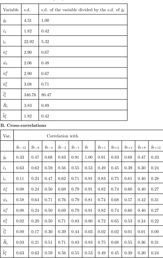
Table 1 reports the results of a stochastic simulation exercise where it was assumed that there are only shocks in the firms’ technological parameter (no shocks in the banks’ technological parameter). The results for the real variables ˆyt, ˆct, ˆıt, ˆnst, and ˆwt are very close to the results we obtained with a zero growth version of the model in King, Plosser and Rebelo (1988) calibrated with our parameters. The results for ˆnd

t are almost exactly the same as the results for ˆnst. This, of course, is a consequence of the market clearing condition in the labour market and of the fact that the weight of the demand for labour by firms is huge when compared with the weight of the demand for labour by banks (see calibration above).

In this stochastic simulation exercise (table 1), the results for bRt, bibtand ˆnbtwere not very good (when we compare them to what the empirical data show). Therefore, we do not discuss these results now. We shall make a detailed comment about the results for these 3 variables in section 9.2.2 (in the context of the stochastic simulation exercise reported in table 2 where the results were much better).

9.2

Technological innovations in the banking sector

We next examine the results of experiments that consider shocks to the banks’s technological parameter (Dt). In order to perform the experiments that follow, we assumed that the banks’ technological parameter evolves according to

b

Dt= 0.9 bDt−1+ ϕt

9.2.1 Impulse Response

Let us now see what happens when at t = 2 a 1% shock occurs in the banks’ technology (with no shock in the firms’ technology). As an example, we can think of shocks in the banks’ technology as the impact that new software has on the productivity of the banks’ employees and infrastructure. With a better designed software, the same amount of hours of work combined with the same infrastructure implies that a higher amount of credit in real terms is processed. This can be modelled as an increase in the parameter Dt. The results are plotted in figures 13 to 24. It is interesting to see that the economy uses the technological gift in the banking industry to improve the general welfare of the people that live in it. We can see that consumption and leisure, the variables that give utility to households, both increase slightly (figures 14 and 16). The total amount of “hours of work” in the banking industry falls by almost 4% (figure 17) and this reduction is used to increase slightly the “hours of work” in the physical output industry (figure 18) and to increase leisure also by a small amount (figure 16). We can see that a shock in Dt also implies a transfer of physical capital from banks to firms (figures 23 and 24). This happens because the more powerful technology in the banking sector means that banks are capable of performing their role using fewer resources. As a consequence, the economy transfers some capital from the banking sector into the sector that produces the goods that directly affect the household’s utility (the nonbank sector). An example from the real world could be internet banking which makes banks sell some branches and offices to other sectors because they have become redundant. In spite of the reduction in the total amount of hours of work in banks and of the fall in the banks’ capital stock, banks are still able to supply a slightly higher amount of credit in real terms (figure 19) because their technology has become more powerful. This slightly higher amount of credit in real terms is necessary to finance the slightly higher amount of consumption.

We can rationalize as follows. When a technological improvement occurs in banks, the amount of credit that the banks can supply with their existing resources increases automatically (through the banks’ production functions). However, bank credit in itself does not give utility to house-holds. Bank credit only becomes useful if used to finance consumption. Therefore, some capital and labour are transferred from banks to firms to allow an increase in output that will permit consumption to rise along with bank credit (the more powerful technology in banks enables them to supply more credit even with fewer resources).

The results we have quoted so far are robust to changes in the parameters. In other words, the qualitative nature of the results does not change when we make reasonable modifications in the

parameters. There is, however, one interesting feature of the model which may be described as follows. It is possible to show that, with the parameter values of section 8, the banking industry is the capital intensive industry. If we change the parameters in a way that makes the banking industry become the labour intensive industry (for example, by setting γ = 0.8), then the results we obtain are qualitatively the same but with two exceptions: the response of the real wage and of the labour supply to a technological improvement in banks. If we ignore period 2 (which is the period where the shock occurs and hence is different from the following periods because capital cannot adjust), then we can say that the effect of a technological innovation in banks is the opposite of the result we have in this paper: the real wage falls and the labour supply also falls. It becomes easy to understand this qualitative change if we take into account that the production structure of our model has the basic Heckscher-Ohlin features (two goods are produced using two factors of production which are perfectly mobile between sectors). We have seen that, when a technological improvement occurs in banks, there is a transfer of capital and labour from banks to firms. When the banking sector is the labour intensive sector, it will release relatively more labour than capital (when compared with the case where the banking sector is the capital intensive sector). This stronger release of work hours will exert downward pressure on the real wage and this will make the labour supply fall.

9.2.2 Stochastic Simulation

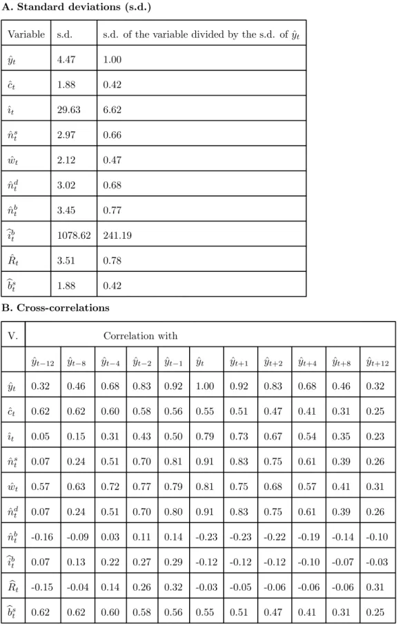
Table 2 reports the results of a stochastic simulation exercise performed assuming that there are shocks in both the firms’ technology (At) and the banks’ technology (Dt). We assume that At evolves according to the process given by 24 and we assume that in each period bDt= bAt.

The only results in table 2 that show a marked change when compared with the results in table 1 are the results for bRt, bibt, ˆnbt and bit. The reason why the other variables are not much affected is as follows. Since the banking industry is very small (see calibration above), the behaviour of the main real variables is determined by the technological shocks outside the banking industry and is not much affected by the technological shocks in the banking industry. The real wage, for example, is mainly determined by the demand for labour by nonbank firms and by the supply of labour by the households. The only important interaction between the two sectors that is caused by the technological shocks in banks is the transfer of physical capital between sectors. For this reason, the only variable outside the banking sector that is affected in an important way by the technological shocks in banks is firms’ investment (bit). On the other hand, the variables that relate directly to the banking industry ( bRt, bibt and ˆnbt) depend a lot on the technical conditions

prevailing in the banking industry itself (as we have seen in the impulse response exercise). Let us compare the results we obtained in table 2 for bRt, bibtand ˆnbt with the results we obtain from the data.

Let us first compare the results we obtained for bRtwith the results from the data. King and Watson (1996) report the following cross-correlations between the interest rate and real output

Variable correlation with

yt−4 yt−3 yt−2 yt−1 yt yt+1 yt+2 yt+3 yt+4 Rt 0.58 0.60 0.57 0.47 0.30 0.07 -0.19 -0.43 -0.61

We can see in table 2 that the correlation coefficients we obtained between bRt andybt,ybt+1, b

yt+2andybt+4are all slightly negative.

Let us now compare the results we obtained for bibt with the results we obtain from the data. Using annual data for the period 1960-1986 and using a Hodrick-Prescott filter to estimate the trends, we have obtained a contemporaneous correlation between “Percentage deviations from trend of real investment in U.S. commercial banks” and “Percentage deviations from trend of Real GDP in fixed 1992 dollars” equal to −0.17. The data were obtained from the BEA cd-rom and fcd-rom the FRED, respectively. With Real GDP in fixed 1992 dollars, the whole set of correlations we obtained for the period 1960-1986 was as follows

Variable Correlation with ˆ

yt−3 yˆt−2 yˆt−1 yˆt yˆt+1 yˆt+2 yˆt+3 bib

t -0.01 0.14 0.05 -0.17 -0.52 -0.56 -0.33 The ratio (standard deviation of bib

t / standard deviation of ˆyt) that we obtain from the data in the period 1960-1986 is 4.11.

After making the necessary adjustments in our model (in the calibration and in the way the shocks are generated) so that the periods in our model can be interpreted as years, we obtained the following correlations in the case of identical and perfectly correlated technological shocks in firms and banks

Variable Correlation with ˆ

yt−3 yˆt−2 yˆt−1 yˆt yˆt+1 yˆt+2 yˆt+3 bib

The ratio (standard deviation of bib

t/ standard deviation of ˆyt) that we obtained with our model was 78.51.

It is interesting to note that some of our simulation results are not very far from the values we obtain from the data. In particular, note that the contemporaneous correlation between bib t and ˆyt that we obtained with our model (−0.18) is close to the value we obtain from the data (−0.17). The two impulse response exercises we have examined make us know that the negative correlation between bibtand ˆytoccurs because both the positive shocks in the firms’ technology and the associated positive shocks in the banks’ technology cause a relocation of capital from banks to firms. On the other hand, with one exception, the correlations between banks’ investment and the past and future values of real output that we obtained with our model have the same sign that they have in the data. Along other dimensions our results are not as good. In particular, although banks’ investment in our model is more volatile than output (as in the data) it seems to be much more volatile in our model than in the real world. This is not surprising because in our model physical capital is homogeneous and there are no adjustment costs.

Let us now compare the results we obtained for ˆnb

t with the results we obtain from the data. Using quarterly data for the period 1972-1986 and using a Hodrick-Prescott filter to estimate the trends, we have obtained a correlation between “Percentage deviations from trend of total hours of work in U.S. commercial banks” and “Percentage deviations from trend of Real GDP in fixed 1992 dollars” equal to −0.158. The data were obtained from the BLSD and from the FRED, respectively. With Real GDP in fixed 1992 dollars, the whole set of correlations we obtained from the data was as follows

Variable Correlation with ˆ

yt−12 yˆt−8 yˆt−4 yˆt−2 yˆt−1 yˆt yˆt+1 yˆt+2 yˆt+4 yˆt+8 yˆt+12 ˆ

nbt 0.37 0.53 0.53 0.22 0.07 -0.16 -0.39 -0.59 -0.77 -0.51 -0.013 The ratio (standard deviation of ˆnb

t / standard deviation of ˆyt) that we obtain from the data is 0.64.

Note that the contemporaneous correlation between ˆnb

tand ˆytthat we obtained with our model in the case of identical and perfectly correlated shocks in banks and firms (which was −0.23 as can be seen in table 2B) is not far from the value we obtain from the data (-0.16). On the other hand, with two exceptions, the correlations between hours of work in banks and the past and future values of real output that we obtained with our model have the same sign that they have in the data. The negative correlations between ˆnb

that we obtained in our model in the case of identical and perfectly correlated shocks in banks and firms (table 2) can be explained as follows. When Atrises, the real income of each household rises which makes them wish to increase consumption. This causes an increase in the demand for credit in real terms. Since the rise in Atis accompanied by a rise in Dt, banks are able to reduce nb

t and still supply more credit in real terms. It is obvious from the impulse response exercises we have examined that this slightly negative correlation could only arise in our model if there are technological shocks in the banking industry. We can also see that the ratio (standard deviation of ˆnb

t / standard deviation of ˆyt) in our model (which is 0.77, as we can see in table 2A) is not far from the value we obtain from the data (0.64).

We can summarize by saying that the results in table 2 reproduce the usual results from RBC models and, at the same time, give us some interesting results in terms of bRt, bibt and ˆnbt.

It is also of interest to compare the correlations between bank credits and real output in our model with the correlations obtained from the data. In our model, the real supply of credit (denoted bs_t) is equal to the value of real money balances. King and Watson (1996) report the following cross-correlations between real money balances and real output

Variable correlation with

yt−4 yt−3 yt−2 yt−1 yt yt+1 yt+2 yt+3 yt+4 ¡_M

P ¢

t 0.07 0.20 0.35 0.49 0.61 0.69 0.71 0.68 0.58

We can see in the last row of table 2B that the correlations we obtain with our model are not far from the correlations that King and Watson obtain from the data. In particular, the contemporaneous correlation between real money and real output in our model (0.55) is quite close to the value obtained in their empirical study (0.61). Let us try to explain why this positive correlation appears in our model. In our model, a positive technological shock implies more physical output and hence higher wage and dividend payments in real terms. Knowing these payments (which will only be made at the end of the period) to be higher, households want to consume more and, therefore, borrow more at the beginning of the period. The banking industry responds to this increased demand for credit by supplying a higher amount of credit in real terms. As a consequence, real output and real credit appear positively correlated.

10

Conclusion

We have built a model which can be used to evaluate the impact of industry-specific technological shocks. As might have been expected, a positive shock in the firms’ technology causes a transfer

of capital from the banking industry to the physical output industry. Less predictable was the fact that a positive shock in the banks’ technology also causes a transfer of capital from the banking industry to the physical output industry. We have explained that this happens because the more powerful technology in the banking sector means that banks can perform their role of suppliers of credit using a lower stock of capital. As a consequence, it is in the interest of the economy as a whole to transfer some capital to the sector that produces the goods that give utility to households (the nonbank sector).

The simulation experiments we performed show the adjustments that are triggered by different combinations of technological shocks when we use a general equilibrium model to represent the economy. Some of the results we obtained were very close to the results we obtain from the data. In particular, in the case of identical and perfectly correlated technological shocks in banks and firms we were able to approximately replicate the contemporaneous correlation between banks’ investment and real output and the contemporaneous correlation between hours of work in banks and real output. On the other hand, with one exception, the cross-correlations between banks’ investment and the past and future values of real output that we obtained have the same sign that they have in the data. Also, with two exceptions, the cross-correlations between hours of work in banks and the past and future values of real output that we obtained have the same sign that they have in the data. Along other dimensions, the results were not as good. In particular, although banks’ investment in our model is more volatile than output (as in the data) it seems to be much more volatile in our model than in the data.

APPENDIX

In this appendix, we explain in detail how the credit-in-advance constraint appears in period 0 and how, under Rational Expectations, it is propagated into future periods. We start by showing that if we add our specific initial condition to the household’s period 0 budget constraint, in equilibrium we obtain a credit-in-advance constraint for period 0. In order to prove this, we start by writing the household’s budget constraint (equation 7) for period t = 0

W₋₁ns₋₁+ f =F_X f =1 z₀fΠf₋₁+ f =F_X f =1 z₀fQf₀+ l=L X l=1 z₀bank,lΠbank,l₋₁ + l=L X l=1 z₀bank,lQbank,l₀ + B1 1 + R0 = = B0+ P0c0+ f =F_X f =1 z₁fQf₀+ l=L X l=1 z₁bank,lQbank,l₀

Using the initial condition before normalization (equation 9) in this last equation yields B1 1 + R0 = P0c0+ f =F_X f =1 Qf₀(zf_{1− z0}f) + l=L X l=1

Qbank,l₀ (z₁bank,l_{− z0}bank,l)

Using the market clearing conditions in the firms’ shares market and in the banks’ shares market in periods (−1) and 0 (which are z0f =H1, z

f 1 =H1, z bank,l 0 = H1 and z bank,l 1 =H1) this last equation becomes B1 1 + R0 = P0c0 (25)

which means that, in equilibrium, the household will have to borrow at the beginning of period 0 an amount equal to the amount she wants to spend buying consumption goods during period 0 (i.e., in equilibrium, there is a credit-in-advance constraint in period 0). Dividing both sides of this equation by P0, we obtain equation 14 for period t = 0.

If we assume Rational Expectations, this credit-in-advance constraint is propagated to all future periods (periods 1,2,3,...). In order to show this, we proceed as follows. By assuming Rational Expectations, we introduce all future budget constraints of the household and all future market clearing conditions into the structure of the mathematical representation of this economy. Hence, we can reason starting from period 0 and going successively into every future period in the following way. We first write the following tautology

B1= B1 1 + R0 (1 + R0) ⇔ B1= B1 1 + R0 + B1 1 + R0 R0

This tautology simply says that the household’s debt at the beginning of period 1 is equal to the principal borrowed at the beginning of period 0 plus interest on it.

Using the credit-in-advance constraint for period 0 which we have just derived (equation 25), this last equation can be written as

B1= P0c0+ B1 1 + R0

R0

Using the market clearing condition in the goods market in period 0, we obtain

B1= F H £ P0A0 F (k0, nd0) − P0 [k1− (1 − δ)k0] ¤ − L H £ P0 [kb1− (1 − δB)k0b] ¤ + B1 1 + R0 R0 Using the definition of nominal profits of firm f in period 0 (equation 4), we obtain

B1= F H h Πf₀+ W0nd0 i −_HL £P0[k1b− (1 − δB)kb0] ¤ + B1 1 + R0 R0⇔ ⇔ B1= W0 F Hn d 0+ F HΠ f 0− L H £ P0 [kb1− (1 − δB)k0b] ¤ + B1 1 + R0 R0 With the market clearing condition in the labour market, this becomes

B1= W0(ns0− L Hn b 0) + F HΠ f 0− L H £ P0 [kb1− (1 − δB)k0b] ¤ + B1 1 + R0 R0 Using the market clearing condition from the bank loans market, we obtain

B1= W0(ns0− L Hn b 0) + F HΠ f 0− L H £ P0 [kb1− (1 − δB)k0b] ¤ + L HB s 0R0 Rearranging, we obtain B1= W0ns0+ F HΠ f 0+ L H £ R0Bs0− W0nb0− P0 [k1b− (1 − δB)kb0] ¤ Using the definition of nominal profits of bank l in period 0 (equation 2), we obtain

B1= W0ns0+ F HΠ f 0+ L HΠ bank,l 0

Finally, using the market clearing conditions in the shares market, this can be written as B1= W0ns0+ f =F_X f =1 z₁fΠf₀+ l=L X l=1 zbank,l₁ Πbank,l₀ (26)

Note that this equation is identical in form to the initial condition we propose using for period t = 0 (equation 9) but written one period ahead. In other words, it is an initial condition for period t = 1. This is an interesting property of the initial condition we propose using: if we assume it holds at the beginning of period 0, then (under Rational Expectations) the structure of the model will automatically reproduce it into the following periods. Combining equation 26 with the household’s budget constraint for period t = 1 and then using the market clearing conditions from the shares market, we obtain

B2 1 + R1

= P1c1

which is a credit-in-advance constraint identical in form to the credit-in-advance constraint for period 0 which we have already obtained (equation 25) but written one period ahead. In other words, it is a credit-in-advance constraint for period t = 1. Dividing both sides of this equation by P1, we obtain equation 14 for period t = 1.

If we repeat the whole reasoning we will also obtain a credit-in-advance constraint for period t = 2. And if we successively repeat the whole reasoning, we will obtain a credit-in-advance constraint for all future periods.

References

[1] Bak, P., Chen, K., Scheinkman, J. and Woodford, M. 1993. Aggregate fluctuations from independent sectoral shocks: self organized criticality in a model of production and inventory dynamics. Ricerche-Economiche 47: 3-30.

[2] Backus, D. and Kehoe, P. 1992. International evidence on the historical properties of business cycles. American Economic Review 82: 864-888.

[3] Barro, R. 1993. Macroeconomics, John Wiley & Sons, Inc.

[4] Blanchard, O. and Khan, M. 1980. The solution to linear difference models under rational expectations. Econometrica 48: 1305-1311.

[5] Burnside, C., Eichenbaum, M. and Rebelo, S. 1996. Sectoral Solow residuals. European Eco-nomic Review 40: 861-869.

[6] Chao, C.-C. and Yip, C. K. 2000. Urban unemployment and optimal trade policy in a cash-in-advance economy. Journal of Economics 71: 59-77.

[7] Horvath, M. 2000. Sectoral shocks and aggregate fluctuations. Journal of Monetary Economics 45: 69-106.

[8] Horvath, M. and Verbrugge, R. 1999. Shocks and sectoral interactions: an empirical investi-gation. Manuscript, Stanford University.

[9] King, R. and Plosser, C. 1984. Money, credit and prices in a real business cycle. American Economic Review 74: 363-80.

[10] King, R., Plosser, C. and Rebelo, S. 1988. Production, growth and business cycles: I. The basic neoclassical model. Journal of Monetary Economics 21: 195-232.

[11] King, R. and Watson, M. 1996. Money, prices, interest rates and the business cycle. Review of Economics and Statistics 78: 35-53.

[12] Kydland, F. and Prescott, E. 1990. Business cycles: real facts and a monetary myth. Quarterly Review. Federal Reserve Bank of Minneapolis, Spring.

[13] Lucas, R., Jr. 1982. Interest rates and currency prices in a two-country world. Journal of Monetary Economics 10: 335-359.

Table 1. Stochastic simulation. Shocks in the firms’ technological parameter. A. Standard deviations (s.d.)

Variable s.d. s.d. of the variable divided by the s.d. of ˆyt ˆ yt 4.31 1.00 ˆ ct 1.82 0.42 ˆıt 22.92 5.32 ˆ ns t 2.90 0.67 ˆ wt 2.06 0.48 ˆ nd t 2.90 0.67 ˆ nb t 3.08 0.71 bib t 346.76 80.47 ˆ Rt 3.83 0.89 bbs t 1.82 0.42 B. Cross-correlations

Var. Correlation with ˆ yt−12 yˆt−8 yˆt−4 yˆt−2 yˆt−1 yˆt yˆt+1 yˆt+2 yˆt+4 yˆt+8 yˆt+12 ˆ yt 0.33 0.47 0.68 0.83 0.91 1.00 0.91 0.83 0.68 0.47 0.33 ˆ ct 0.63 0.62 0.59 0.56 0.55 0.53 0.49 0.45 0.39 0.30 0.24 ˆıt 0.11 0.24 0.47 0.62 0.71 0.91 0.83 0.75 0.61 0.40 0.28 ˆ ns t 0.08 0.24 0.50 0.69 0.79 0.91 0.82 0.74 0.60 0.40 0.27 ˆ wt 0.58 0.64 0.71 0.76 0.79 0.81 0.74 0.68 0.57 0.42 0.31 ˆ nd t 0.08 0.24 0.50 0.69 0.79 0.91 0.82 0.74 0.60 0.40 0.27 ˆ nb_t 0.02 0.20 0.50 0.71 0.83 0.80 0.72 0.65 0.53 0.34 0.22 bib t 0.09 0.17 0.30 0.39 0.44 0.03 0.02 0.02 0.01 0.01 0.00 b Rt 0.03 0.21 0.51 0.71 0.83 0.83 0.75 0.68 0.55 0.36 0.31 bbs t 0.63 0.62 0.59 0.56 0.55 0.53 0.49 0.45 0.39 0.30 0.24

Table 2. Stochastic simulation. Identical and perfectly correlated shocks in the firms’ technological parameter and in the banks’ technological parameter.

A. Standard deviations (s.d.)

Variable s.d. s.d. of the variable divided by the s.d. of ˆyt ˆ yt 4.47 1.00 ˆ ct 1.88 0.42 ˆıt 29.63 6.62 ˆ ns t 2.97 0.66 ˆ wt 2.12 0.47 ˆ nd t 3.02 0.68 ˆ nb t 3.45 0.77 bib t 1078.62 241.19 ˆ Rt 3.51 0.78 bbs t 1.88 0.42 B. Cross-correlations V. Correlation with ˆ yt−12 yˆt−8 yˆt−4 yˆt−2 yˆt−1 yˆt yˆt+1 yˆt+2 yˆt+4 yˆt+8 yˆt+12 ˆ yt 0.32 0.46 0.68 0.83 0.92 1.00 0.92 0.83 0.68 0.46 0.32 ˆ ct 0.62 0.62 0.60 0.58 0.56 0.55 0.51 0.47 0.41 0.31 0.25 ˆıt 0.05 0.15 0.31 0.43 0.50 0.79 0.73 0.67 0.54 0.35 0.23 ˆ ns_t 0.07 0.24 0.51 0.70 0.81 0.91 0.83 0.75 0.61 0.39 0.26 ˆ wt 0.57 0.63 0.72 0.77 0.79 0.81 0.75 0.68 0.57 0.41 0.31 ˆ nd_t 0.07 0.24 0.51 0.70 0.80 0.91 0.83 0.75 0.61 0.39 0.26 ˆ nb t -0.16 -0.09 0.03 0.11 0.14 -0.23 -0.23 -0.22 -0.19 -0.14 -0.10 bib t 0.07 0.13 0.22 0.27 0.29 -0.12 -0.12 -0.12 -0.10 -0.07 -0.03 b Rt -0.15 -0.04 0.14 0.26 0.32 -0.03 -0.05 -0.06 -0.06 -0.06 0.31 bbs t 0.62 0.62 0.60 0.58 0.56 0.55 0.51 0.47 0.41 0.31 0.25