Effect of loan value and collateral on value of mortgage default

Int. J Latest Trends Fin. Eco. Sc. Vol‐3 No. 4 December, 2013

Effect of Loan Value and Collateral

on Value of Mortgage Default

Rais Ahmad Itoo #1_{, Selvarasu Appasamy Mutharasu}#2_{, José António Filipe}* #

Annamalai University, India

1_{raisitoophd@yahoo.com} 2_{aselvarasu@gmail.com}

*_{Instituto Universitário de Lisboa (ISCTE-IUL), BRU – IUL}

Lisbon, Portugal

jose.filipe@iscte.pt

Abstract

:

Keywords – Mortgage Default, Loan value contents, Collateral, LTV, LTI, Logistic regression.

1.

Introduction

First, in this study, it is necessary to consider some fundamental aspects of the core ideas to be presented. Mortgage system of financial service in general, the mortgage loan market in India and mortgage default will be considered next for the first insights.

Mortgage System of Financial Service - In the

beginning, a mortgage was just a conveyance of land for a fee. The buyer paid the seller a set rate, with no interest, and the seller would sign over the land to the buyer. There were usually conditions to be met before the land to become property of the buyer, just as happens today, but usually it was based upon the assumption that the land would produce the money to be paid back to the seller. So, a mortgage was written due to this fact. The mortgage was kept in effect no matter the land was producing or not. This old arrangement was very lopsided once the seller of the property - or the lender who was holding the deed to the land - had absolute power over it and could do whatever he liked, including selling it, not allowing payment, refusing payoff, among other possibilities which caused major problems to the buyer, who held no ground at all. With time, and blatant abuse of the mortgage system, the courts began to uphold more of the buyers' rights, so that they had more to stand on when they came to become owners of their land. Eventually, they were allowed to demand the deed to be free and clear upon the payoff of the property. There were still several steps to be taken to ensure that the seller still had enough rights to keep his interest safe and make sure that his money would be paid.

Although mortgages have changed from one form to another, but still the essentials of contract are same. Now, there are many more laws and regulations to help to protect the buyer, but also the seller and the creditor. There are also many different ways to lock in a low interest rate, borrower just need ____________________________________________________________________________________

International Journal of Latest Trends in Finance & Economic Sciences IJLTFES, E‐ISSN: 2047‐0916

Int. J Latest Trends Fin. Eco. Sc. Vol‐3 No. 4 December, 2013 to talk to mortgage broker about what the rates are

now and what kinds of programs they offer to keep those interest rates low throughout the life of borrower’s loan.

A mortgage is an agreement of security so that borrowers have to pay the debt. In many cases, the borrower will give up collateral security if he/she fails to repay the loan as agreed. Mortgage can be used as a verb, meaning “to pledge”. Mortgage and “home loan” are often used interchangeably. However, the mortgage is really the agreement that makes home loan to work. The bank would not lend the borrower hundreds of thousands of dollars unless the bank knew that it would be possible to claim collateral security in the event of mortgage default. A loan to finance the purchase of a real estate usually requires specified payment periods and interest rates. The borrower gives the lender (mortgagee) a lien on the property as collateral for the loan.

Mortgage financing is an essential decision for both, borrowers and lenders. Not only this decision is qualitatively important, it is quantitatively significant, as well. The aggregate outstanding mortgage balances, and thus the capitalization of various mortgage related securities, is in the trillions. No wonder that the various aspects of mortgage contracting have been one of the most extensively researched topics in real estate finance and economics, both theoretically and empirically. Amongst these aspects, mortgage default has been one of the leading topics. Understanding mortgage default is necessary for appropriately valuing mortgages and for borrowers and lenders optimization. In most countries, a mortgage is the primary way that prospective homeowners have of buying a house, flat or land on which to build a property, collectively called real estate. This type of mortgage is called a residential mortgage or home loan. They are most often taken up by individuals or couples.

A mortgage loan is a loan secured by real property through the use of a mortgage note which evidences the existence of the loan and the encumbrance of that realty through the granting of a mortgage which secures the loan. However, the word mortgage alone, in everyday usage, is most often used to mean mortgage loan. A home buyer or builder can obtain financing (a loan) either to

purchase or to secure against the property from a financial institution, such as a bank, either directly or indirectly through intermediaries. Features of mortgage loans such as the size of the loan, maturity of the loan, interest rate, method of paying off the loan, and other characteristics can vary considerably.

In many jurisdictions, though not all, it is normal for home purchases to be funded by a mortgage loan. Few individuals have enough savings or liquid funds to enable them to purchase property outright. In countries where the demand for home ownership is high, strong domestic markets have developed. The word mortgage is a French term meaning "dead pledge," apparently meaning that the pledge ends (dies) when either the obligation is fulfilled or the property is taken through foreclosure.

Mortgage Loan Market: the Indian Scenario

- Indian Mortgage Market is one of the largest divisions in the banking financial services and insurance sector. The India Mortgage Market was previously known as the Indian housing finance industry. At present the total worth of the India Mortgage Market is nearly US $ 18 billion. The gross domestic product to mortgage ratio in India is very low in comparison to other developed countries. The ratio in the foreign countries ranges from 25% to 60% whereas in India the ratio is 2.5%. The India Mortgage Market is showing fast growth in the past few years. The foremost players in this sector are the finance corporation but presently the commercial banks are also starting to play an important role in the development and growth of the India Mortgage Market. At present the market leader in the India mortgage market is the Housing Development Finance Corporation (HDFC), with the State Bank of India (SBI) following the leader.

Mortgage Default - The situation in which

borrower is not making payments on his or her mortgage loan is called mortgage default and the loan is considered to be “in default,” meaning that the agency which holds the note can choose to take over the property. In finance, default occurs when a debtor has not met his or her legal obligations according to the debt contract, e.g. has not made a scheduled payment, or has violated a condition of the debt contract. A default is the failure to pay back a loan. Default may occur if the debtor is either unwilling or unable to pay his or her debt. This can

Int. J Latest Trends Fin. Eco. Sc. Vol‐3 No. 4 December, 2013 occur with all debt obligations including bonds,

mortgages, loans, and promissory notes.

The term default must be distinguished from the terms insolvency and bankruptcy. Default essentially means a debtor is not repaying the debt which he or she is required to have to pay. Insolvency means that debtor does not have ability to repay the debt and Bankruptcy is a legal finding that imposes court supervision over the financial affairs of those who are insolvent or in default.

Default can be of three types: 1. Technical default, 2. Strategic default, 3. Debt services default.

Technical default occurs when an affirmative or a negative covenant is violated. Affirmative covenants are clauses in debt contracts that require firms to maintain certain levels of capital or financial ratios. The most commonly violated restrictions in affirmative covenants are tangible net worth, working capital /short term liquidity, and debt service coverage. Negative covenants are clauses in debt contracts that limit or prohibit corporate actions e.g. sale of assets, payment of dividends, that could impair the position of creditors. Negative covenants may be continuous or incurrence-based. Violations of negative covenants are rare compared to violations of affirmative covenants.

When a debtor chooses to default on a loan, despite being able to make payments, this is said to be a strategic default. This is most commonly done for non-recourse loans, where the creditor cannot make other claims on the debtor; a common example is a situation of negative equity on mortgage loan in common law jurisdictions such as in the United States, which is in general “non-recourse”. In this case, default is colloquially called “jingle mail”, the debtor stops making payments and mails the keys to the creditor, generally a bank.

When the borrower has not repaid the interest or principal which he/she was supposed to repay, it is called debt service default. Defaulting on a mortgage can result in the loss of a collateral security and accordingly it must be avoided. Even if the collateral security is not lost to the bank, a mortgage default will drag down a credit score significantly, making it

harder to negotiate with the bank or to secure credit for other loans in the future. When a mortgage loan is issued, a monthly due date for payments is usually specified. Many mortgages include a grace period of from one to two weeks, meaning that payments sent during the grace period will still be considered on time. After the grace period has elapsed, however, late fees will start to be levied. If more than 30 days after the due date go by, the mortgage is considered to be in default. Once the bank determines that the 30 days have elapsed, it sends a notice of mortgage default to a credit agency, impacting the credit score immediately. Within weeks, the bank will usually retain the services of a credit collection agency in an attempt to get the homeowner's past due payments. This adds to the fees associated with mortgage default. Many banks will also insist on a full payment including late fees and collection fees to bring the homeowner current, and they will not accept partial mortgage payments when the mortgage is in default. Within 60 to 90 days of the determination that the mortgage has defaulted, the bank will send a notice of mortgage default to the homeowner. This is the first step in foreclosure proceedings, giving the property owner a chance to make up the missed payments immediately and in full, or to risk having the collateral security taken over by the bank and sold at auction. The bank will also be obliged to post a public notice about the foreclosure, and the property owner will have a chance to buy the property back during the foreclosure auction, if he or she can muster up the funds in cash. Some people choose to default on their mortgages and simply walk away, deciding that the negative impact on their credit scores is better than sinking any more equity into the home. This is most common in areas where property values have declined radically, leaving people with loans which are larger than their homes are worth. Other people may try to sell their homes before their mortgages go into default so that they can wipe the slate and start over again.

For homeowners who think that they may be risking mortgage default, the best thing to do is to talk to the lender. Ignoring payment notices, phone calls, and legal notices is not advisable, because the bank will refuse to negotiate with property owners who have not been proactive. Immediately as a property owner, he thinks that a mortgage payment will be missed, he or she shall contact the lender to

Int. J Latest Trends Fin. Eco. Sc. Vol‐3 No. 4 December, 2013 negotiate. Many lenders are willing to offer a longer

grace period, or to permit reduced payments due to financial hardship to avoid mortgage default, as the bank would rather not deal with the hassle of a foreclosure auction. A history of paying on time and handling the mortgage responsibly will make the bank more likely to cooperate.

2.

Review of Literature

This section deals with the dependent and independent variables and deals with other category of mortgage outstanding amount and related parameters of the study. The variables in this section are age, marital status, gender, educational qualification, monthly income, value of collateral security, purpose of loan, loan amount, mortgage outstanding balance, interest rate, loan type, type of collateral security, unemployment, loan-to-value ratio (LTV) and loan-to-income ratio (LTI). The studies involving mortgage loan have been reviewed and description of all variables are presented.

2.1 The age of the borrower

Capozza et al. (1997) indicated that the borrower’s age was negatively correlated with the default probability. Hakim and Haddad (1999) studied the influences of the borrower’s attributes and the loan characteristics on the mortgage loan default using a failure-time model. Their results indicated that the age of the borrower is significantly negatively correlated with the default probability. Jacobson and Roszbach (2003) indicated the applicant’s age was significantly negatively correlated with the unsecured loan default. Cairney and Boyle (2004) showed that the age of the borrower was significantly negatively correlated with the default risk of credit loans. Von Furstenberg and Green (1974) and Avery et al. (2004) in their studies they have assessed local situational factors as factors of default risk. They found that inclusion of a situational factor like the age of the borrower improves the performance of the scoring models. Orla and Tudela (2005) found that persistence in mortgage payment problems was greater among households in which the head’s age was 35 years old , or over than it was among households headed by younger individuals. The younger households are more capable of getting out of problems than those aged 35 or over. Kumar (2010) found that there is no

significance between the age of the borrower and mortgage defaults.

2.2 Marital Status of borrower

Von Furstenberg and Green (1974), Avery et al. (2004) in their studies they have assessed local situational factors as factors of default risk. They found that inclusion of situational factor like marital status of borrower improves the performance of the scoring models. Cairney and Boyle (2004) showed that the marital status (single, widowed, or divorced) was significantly positively correlated with the default risk of credit loans.

2.3 Gender of borrower

Jacobson and Roszbach (2003) indicated that the applicant’s gender was significantly negatively correlated with the unsecured loan default.

2.4 Borrower’s Educational Qualification Liu and Lee (1997) presented that the borrower’s education degree was significantly negatively correlated with the mortgage loan default. Cairney and Boyle (2004) showed whether the education level was significantly negatively correlated with the default risk of credit loans.

2.5 Monthly Income of Borrower

Stansell and Millar (1976), Vandell (1978), Ingram and Frazier (1982) have found that payment-to-income ratio is positively correlated with the probability of default i.e. higher the payment to income ratio, greater is the default risk. Clauretie (1987) has also argued that other non-equity factor like sources of income play a larger role in affecting default levels. Capozza et al. (1997) indicated that the income was negatively correlated with the default probability. Hakim and Haddad (1999) studied that the disposable income was negatively correlated with the default probability. Jacobson and Roszbach (2003) indicated that the annual income from wages was significantly positively correlated with the unsecured loan default. Cairney and Boyle (2004) showed that the borrower’s income was significantly negatively correlated with the default risk of credit loans. Har and Eng (2004) also showed that the income was negatively correlated with the mortgage loan default. Teo and Ong (2005) indicated that the income was positively correlated with the mortgage loan default.

Int. J Latest Trends Fin. Eco. Sc. Vol‐3 No. 4 December, 2013 2.6 Value of Collateral Security

Vandell and Thibodeau (1985) used a simulation analysis to demonstrate several non-equity factors overshadowing the equity effect on default which explained about households with zero or negative equity did not default, while others with positive equity. Clauretie (1987) has also argued that other non-equity factor like property value played a large role in affecting default levels. The default imposes personal costs on borrowers that include limits on occupational and credit opportunities, social stigma and damage to reputation (Kau, Keenan and Kim, (1993) and Vandell and Thibodeau, (1985)). The costs exceed the absolute value of negative equity. The borrower will not default when Paul Bennett et al. (1997) found that the structural change in the mortgage market had increased homeowners’ propensity to refinance. Bajari et al. (2008) studied empirically the relative importance of the various drivers behind subprime borrower’s decision to default. They emphasize the role of the nationwide decrease in home prices as the main driver of default. Foote et al. (2008) examined homeowners in Massachusetts who had negative home equity during the early 1990s and found that fewer than 10% of these owners eventually lost their home to foreclosure.

2.7 Type of Collateral Security

Teo and Ong (2005) indicated that the collateral type was significantly positively correlated with the mortgage loan default. Yildiary Yildirium (2007) found that loans within the same geographical area and property type tend to exhibit correlation in default incidence.

2.8 Purpose of Loan

Lee (2002) has identified the ‘purpose of purchasing real estate property' is one of the key determinants of default risk. Therefore, when the market price of collateral falls sharply or economic performance becomes much worse, the property frequently is abandoned by the owners thereby limiting their loss. Har and Eng (2004) showed that the use purpose of collateral was negatively correlated with the mortgage loan default.

2.9 Loan Amount

Paul Bennett et al. (1997) found that loan size is negatively correlated with the mortgage defaults. Hakim and Haddad (1999) studied the influences of the borrower’s attributes and the loan characteristics on the mortgage loan default using failure-time model. Their results indicated that the loan amount was negatively correlated with the default probability.

2.10 Interest Rate of loan amount borrowed

Campbell and Dietrich (1983) showed that the interest rates significantly explain mortgage prepayment, delinquencies and defaults by using logit model. Har and Eng (2004) showed that the loan interest rate was significantly positively correlated with the mortgage loan default. Teo and Ong (2005) indicated that the interest rate was significantly negatively correlated with the mortgage loan default. Danny (2008) indicated that any empirical test of the relation between the LTV ratio and the default risk incorporated the interrelationship among the LTV ratio, credit score and interest rate.

2.11 Loan Type

Smith et al. (1996) found that the default probability was significantly affected by the loan type.

2.12 Loan-to-value ratio (LTV)

Campbell and Dietrich (1983) showed that the LTV ratio explain mortgage prepayment. Lawrence et al. (1992) stated that the default risk was positively correlated with the ratio of loan amount to collateral. Smith et al. (1996) found that the default probability was significantly affected by the loan-to-value (LTV) ratio. Liu and Lee (1997) presented that the LTV ratio were significantly positively correlated with the mortgage loan default. Capozza et al. (1997) indicated that the LTV ratio was an important factor affecting the mortgage loan default. Kau and Keenan (1998) treat the default as a rational decision and their research paper provides the entire distribution of defaults’ severity. The distributions of severity are both disperse and skewed. The severity distribution shifts more than in proportion to the rise in the loan to value (LTV) ratio. Further, the researchers have demonstrated that severity of default rises as the LTV ratio increases. According to empirical model, negative mortgage value motivates financial defaults.

Int. J Latest Trends Fin. Eco. Sc. Vol‐3 No. 4 December, 2013 The mortgage value is equity (the amount paid by the

borrower from his savings to the developer apart from bank loan and some more investments in the house for furniture & fittings, registration cost, etc.), house value less mortgage balance, and the value of prepayment and default options imbedded in mortgage contract. Archer et al. (1999) option-based models of mortgage default posit that the central measure of default risk is the loan-to-value (LTV) ratio. Results show that the mortgages with low and moderate LTVs may be as likely to default as those with high LTVs. Archer et al. (2001) argue that LTV at origination is an endogenous risk measure and therefore no empirical relationship between LTV and mortgage default should exist. Ambrose and Sanders (2001) use a competing risks model to examine default and prepayment behavior using 4,257 commercial loans underlying 33 CMBS deals. They also found no statistical relationship between original LTV and default. In their model, however, no measure of property cash flow is included.

Loan-to-income ratio (LTI)

Campbell and Cocco (2010) showed that mortgage default is triggered by negative home equity, which results from declining house prices in a low inflation environment with large mortgage balances outstanding. The level of negative home equity that triggers default depends on the extent to which households are borrowing constrained. High loan-to-value ratios at mortgage origination increase the probability of negative home equity. High loan-to-income (LTI) ratios also increase the probability of default by making borrowing constraints more severe. Interest-only mortgages trade of an increased probability of negative home equity against a relaxation of borrowing constraints.

3.

Research Methodology

This section includes the statement of the problem, presents arguments for the need for the study, the objectives, data collection, sampling, statistical tools; proposition and the limitations of the study. The description of all these aspects of methodology follows.

3.1 Statement of the Problem

In changing economic conditions customers are not able to foresee their income and value of their own property. It is because of the existence of limited

sources of information available to them. When the customer income and their property value decreases, it is likely to result in mortgage default. Companies try to maximize their returns in various means of charges on mortgage loan. The increased charges of banks lead to mortgage default. Mortgage default has an additional cost of transaction for both lender as well as borrower. The different factors which are responsible for mortgage default are payment records, the ratio of loan amount to collateral value and the ratio of the borrower’s income to expenditure (Lawrence et al. 1992), loan-to-value ratio, length of loan, the fluctuation rate of housing price, unemployment rate, divorce rate, and the borrower’ moving frequency (Capozza et al. 1997; Liu and Lee, 1997) percentage of first loan, the loan interest rate, the floor area, and the borrower’s credit risk (Har and Eng, 2004) and whether the borrower’s house is owned by himself or rented, the marital status (single, widowed, or divorced), the degree of living pressure, and the borrower’s credit risk ( Cairney and Boyle, 2004). In effect, the mortgage default is on the rise due to piling up of various reasons in personal risk, loan value and collateral security.

3.2 Need for the Study

In this study, researchers have attempted to evaluate three pronged approach of important dimensions which directly or indirectly affect mortgage default. The effect of borrowers’ profile, loan value and collateral security on mortgage default are studied. Therefore the present study is an effort to bring an understanding of the existing situation with respect to mortgage default. This study aims to evaluate the procedure that facilitates the existing mortgage loan borrowers and also in time with bank’s policy. Also the suggestions take care of customer in order to manage mortgage defaults. 3.3 Objectives of the Study

This work aims:

1. To study the impact of borrower’s profile on mortgage default.

2. To measure the association of borrower profile, loan value and realty of collateral security on mortgage defaulters’ outstanding balance.

Int. J Latest Trends Fin. Eco. Sc. Vol‐3 No. 4 December, 2013 3. To assess relationship of loan value,

collateral security and outstanding balance. 4. To find out the difference between the

present market value of collateral security against outstanding balance of mortgage defaulters.

5. To extrapolate the reason for mortgage default due to socio-economic variables, interest rate, loan schemes, use of loan, secondary finance, loan-to-value ratio and loan-to-income ratio.

3.4 Research Design

The study is a descriptive research about mortgage default. A mortgage default is a situation in which borrower is not making payment on his/her loan. The variables used in this study are categorized into three dimensions: borrower profile, loan value and collateral security. Borrower profile includes age, marital status, gender, educational qualification and income of borrower. Loan value includes loan amount, loan amount repaid, outstanding balance, interest rate, loan type, loan-to-value ratio (LTV), loan-to-income ratio (LTI) and purpose of loan. By its side collateral security includes value of security, type of security and secondary finance.

3.5 Data Collection Design

The whole study is based on extracted data collected from Jammu and Kashmir Bank ltd. from secondary sources maintained in bank but not published. The collected data is from those borrowers who have been declared as defaulters from April 2011 up to March 2012. One of the researchers has spent twenty days in the bank in order to understand the problem in depth and to understand suitability and reliability of data. This researcher has recorded the data from the default borrower’s file. Details about all the variables for the whole sample size are collected.

3.6 Sampling Design

The systematic sampling methods have been adopted to select sample defaulters. The total number of defaulters was 578, out of which 115 is taken as sample. Every fifth borrower was chosen. Due to more variation of data from average value 15 cases of

the sample were eliminated in order to maintain proper intervals. The study area is Jammu and Kashmir and sample unit is mortgage defaulters. The study period spread from September 2011 to August 2012. Sample size is calculated based upon the scale given by Aaker et al. (2009). Co-efficiency of variance for loan-to-value (LTV) has been computed for 30 cases as a pilot study. The computed value is 0.19 and based on this value sample of 99 was taken. 3.7 Statistical Design

The researchers have adopted relevant statistical tools for analysis of data describing mortgage loan defaulters. The following are the relevant tools used for analysis of data viz., chi-square, correlation, regression, ANOVA, paired ‘t’ test and logistic regression have been selected for the proper of analysis of data. SPSS 17.0 is used for the analysis of all the above statistical tools and tabulation of processed data.

3.8 Propositions

P1: Average amount of default loan is not varying with the loan value, property market value directly and the collateral security, secondary finance, socio-economic variables, marital status, gender and age of both commercial and residential borrowers indirectly.

P2: The amount of default loan is not significantly associated with the loan value, property market value directly and the collateral security, secondary finance, socio-economic variables, marital status, gender and age of both commercial and residential borrowers indirectly.

P3: The amount of default loan has no linear relationship with the loan value, property market value directly and the collateral security, secondary finance, socio-economic variables, marital status, gender and age of both commercial and residential borrowers indirectly.

3.9 Limitations of the Study

Bank kept some of borrower’s information confidential. The confidential data maintained by banks, especially contact details were not provided to the researchers. The area of borrower was not available for research and therefore it was difficult to denote the geographic location where there was loan default. Researchers want to study as much data as

Int. J Latest Trends Fin. Eco. Sc. Vol‐3 No. 4 December, 2013 possible in order to identify replication of results.

This was not supported for completion. Electronic softcopy of data was sought by researcher, but it was not permitted to him. The crosscheck of data collection was done by the researcher and not by the bank.

4.

Analysis and Interpretation

The dimensions viz. borrowers profile, loan value contents and characteristics of collateral security have been tested for relationship with borrowers outstanding loan balance by applying correlation test.

4.1 Correlation Analysis

Correlation test between borrower’s profile and outstanding balance

The borrower profile consists of five variables as age, gender, marital status, educational qualification and monthly income of borrower. Correlation method had been applied to find out the relationship between borrower’s profile variables and defaulters outstanding balance. The description of correlation results for each pair is given as follows.

The value of correlation co-efficient between outstanding balance and the age of the borrower “r”=0.308 indicates that 30.8% of the variation in outstanding balance is explained by the age of the borrower. And p value is <0.01 so, there exists a positive relationship between the outstanding balance and age at 99% level of confidence. The value of correlation co-efficient between outstanding balance and educational qualification of borrower “r”=-0.088 indicates that 8.8% of the variation in outstanding balance is explained by the age of the borrower. And p value is >0.05 so, there exists a very weak relationship between the outstanding balance and educational qualification at 95% level of confidence. The value of correlation co-efficient between outstanding balance and gender of borrower “r”=0.196 indicates that 19.6% of the variation in outstanding balance is explained by the age of the borrower. And p value is >0.05 so, there exists a very weak relationship between the outstanding balance and gender at 95% level of confidence. The value of correlation co-efficient between outstanding balance and marital status “r”=0.385 indicates that 38.5% of the variation in outstanding balance is explained by

the marital status of the borrower. And p value is <0.01 so, there exists a positive relationship between the outstanding balance and marital status of borrower at 99% level of confidence. The value of correlation co-efficient between outstanding balance and monthly income “r”=0.539 indicates that 53.9% of the variation in outstanding balance is explained by the monthly income of the borrower. And p value is <0.01 so, there exists a positive relationship between the outstanding balance and monthly income of borrower at 99% level of confidence. (Table 1)

Correlation test between loan contents and outstanding balance

The loan content dimension consists of four variables as loan amount, amount repaid, loan-to-value ratio and loan-to-income ratio. Correlation method had been applied to find out the relationship between loan content variables and defaulters outstanding balance. The description of correlation results for each pair is given as follows.

The value of correlation co-efficient between outstanding balance and interest rate “r”=0.424 indicates that 42.4% of the variation in outstanding balance is explained by interest rate. And p value is <0.01 so, there exists a positive relationship between the outstanding balance and interest rate at 99% level of confidence. The value of correlation co-efficient between outstanding balance and type of loan “r”=-0.155 indicates that 15.5% of the variation in outstanding balance is explained by the type of the loan. And p value is >0.05 so, there exists a very weak negative relationship between the outstanding balance and type of loan at 95% level of confidence. The value of correlation co-efficient between outstanding balance and loan amount “r”=0.847 indicates that 84.7% of the variation in outstanding balance is explained by the loan amount. And p value is <0.01 so, there exists a positive relationship between the outstanding balance and loan amount at 99% level of confidence. The value of correlation co-efficient between outstanding balance and loan amount repaid “r”=0.036 indicates that 3.6% of the variation in outstanding balance is explained by the loan amount repaid. And p value is >0.05 so, there exists very weak relationship between the outstanding balance and loan amount repaid at 95% level of confidence. The value of correlation co-efficient between outstanding balance and

loan-to-Int. J Latest Trends Fin. Eco. Sc. Vol‐3 No. 4 December, 2013 value ratio “r”=0.557 indicates that 55.7% of the

variation in outstanding balance is explained by loan-to-value ratio. And p value is <0.01 so, there exists a positive relationship between the outstanding balance and loan-to-value ratio at 99% level of confidence. The value of correlation co-efficient between outstanding balance and loan-to-income ratio “r”=0.371 indicates that 37.1% of the variation in outstanding balance is explained by loan-to-income ratio. And p value is <0.01 so, there exists a positive relationship between the outstanding balance and loan-to-income ratio at 99% level of confidence. (Table 2)

Correlation test between outstanding balance and collateral security characteristics

The collateral security characteristics consist of three variables as form of security, value of security and secondary finance. Correlation method had been applied to find out the relationship between collateral security variables and defaulters outstanding balance. The description of correlation results for each pair is given as follows.

The value of correlation co-efficient between outstanding balance and type of security “r”=0.209 indicates that 20.9% of the variation in outstanding balance is explained by type of security. And p value is <0.05 so, there exists a positive relationship between the outstanding balance and type of security at 95% level of confidence. The value of correlation co-efficient between outstanding balance and value of property “r”=0.602 indicates that 60.2% of the variation in outstanding balance is explained by value of property. And p value is <0.01 so, there exists a strong positive relationship between the outstanding balance and value of property at 99% level of confidence. The value of correlation co-efficient between outstanding balance and secondary finance “r”=0.099 indicates that 9.9% of the variation in outstanding balance is explained by secondary finance. And p value is >0.05 so, there exists a very weak relationship between the outstanding balance and secondary finance at 95% level of confidence. The value of correlation co-efficient between outstanding balance and use of loan “r”=0.048 indicates that 4.8% of the variation in outstanding balance is explained by use of loan. And p value is >0.05 so, there exists a very weak relationship between the outstanding balance and use of loan at 95% level of confidence. (Table 3)

4.2 ANOVA Analysis

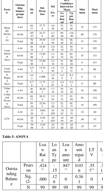
The variables viz. income, loan amount, LTV, value of collateral security and loan amount repaid has been tested for equality of mean with borrower’s outstanding balance by applying ANOVA.

Outstanding Loan Balance Based on Monthly Income

Mean and S.D. based on outstanding loan balance and monthly income have been studied. The results of ANOVA tabulation (table 4) consist of two categories of outstanding loan balance 4-44lacs and 44-84lacs. The result of the study shows that there is a significant difference in the mean score for outstanding loan balance for different categories of borrower based on monthly income. In order to test the group variation in mean scores, a null hypothesis was proposed.

HO: Means of outstanding loan balance is not

significantly influenced by monthly income.

HA: Means of outstanding loan balance is

significantly influenced by monthly income.

In order to test the hypothesis, ANOVA test has been applied (Table 5). It has been found that F value is 34.536 and the ‘p’ value for the level of significance is 0.000. As the ‘p’ value is less than 0.01, it indicates that alternative hypothesis is accepted as outstanding loan balance is significantly influenced by monthly income at 99% level of confidence.

Outstanding Loan Balance Based on Loan Amount

Mean and S.D based on outstanding loan balance and loan amount have been studied. The results of ANOVA tabulation (table 4) consist of two categories of outstanding loan balance 4-44lacs and 44-84lacs. The result of the study shows that there is a significant difference in the mean score for outstanding loan balance for different categories of borrower based on loan amount. In order to test the group variation in mean scores, a null hypothesis was proposed.

HO: Means of outstanding loan balance is not

significantly influenced by loan amount.

HA: Means of outstanding loan balance is

Int. J Latest Trends Fin. Eco. Sc. Vol‐3 No. 4 December, 2013 In order to test the hypothesis, ANOVA test has

been applied (Table 5). It has been found that F value is 65.503 and the ‘p’ value for the level of significance is 0.000. As the ‘p’ value is less than 0.01, it indicates that alternative hypothesis is accepted as outstanding loan balance is significantly influenced by loan amount at 99% level of confidence.

Outstanding Loan Balance Based on Loan Amount Repaid

Mean and S.D based on outstanding loan balance and loan amount repaid have been studied. The results of ANOVA tabulation (table 4) consist of two categories of outstanding loan balance 4-44lacs and 44-84lacs. The result of the study shows that there is a significant difference in the mean score for outstanding loan balance for different categories of borrower based on loan amount repaid. In order to test the group variation in mean scores, a null hypothesis was proposed.

HO: Means of outstanding loan balance is not

significantly influenced by loan amount repaid. HA: Means of outstanding loan balance is

significantly influenced by loan amount repaid. In order to test the hypothesis, ANOVA test has been applied (Table 5). It has been found that F value is 0.039 and the ‘p’ value for the level of significance is 0.844. As the ‘p’ value is greater than 0.05, it indicates that null hypothesis is accepted as outstanding loan balance is not significantly influenced by loan amount repaid at 95% level of confidence.

Outstanding Loan Balance Based on Value of Security

Mean and S.D based on outstanding loan balance and value of security have been studied. The results of ANOVA tabulation (table 4) consist of two categories of outstanding loan balance 4-44lacs and 44-84lacs. The result of the study shows that there is a significant difference in the mean score for outstanding loan balance for different categories of borrower based on value of security. In order to test the group variation in mean scores, a null hypothesis was proposed.

HO: Means of outstanding loan balance is not

significantly influenced by value of security.

HA: Means of outstanding loan balance is

significantly influenced by value of security.

In order to test the hypothesis, ANOVA test has been applied (Table 5). It has been found that F value is 41.374 and the ‘p’ value for the level of significance is 0.000. As the ‘p’ value is less than 0.01, it indicates that alternative hypothesis is accepted as outstanding loan balance is significantly influenced by value of security at 99% level of confidence.

Outstanding Loan Balance Based on Loan-to-Value Ratio (LTV)

Mean and S.D based on outstanding loan balance and LTV have been studied. The results of ANOVA tabulation (table 4) consist of two categories of outstanding loan balance 4-44lacs and 44-84lacs. The result of the study shows that there is a significant difference in the mean score for outstanding loan balance for different categories of borrower based on LTV. In order to test the group variation in mean scores, a null hypothesis was proposed.

HO: Means of outstanding loan balance is not

significantly influenced by LTV.

HA: Means of outstanding loan balance is

significantly influenced by LTV.

In order to test the hypothesis, ANOVA test has been applied (Table 5). It has been found that F value is 13.471 and the ‘p’ value for the level of significance is 0.000. As the ‘p’ value is less than 0.01, it indicates that alternative hypothesis is accepted as outstanding loan balance is significantly influenced by LTV at 99% level of confidence.

4.3 Logistic Regression

Strength of relationship between outstanding balance with age, income, educational qualification, LTV, interest rate, purpose of loan and secondary finance has been studied.

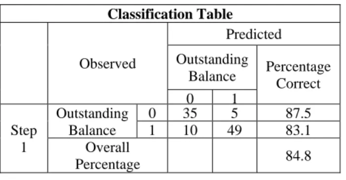
Accuracy is measured as correctly classified records in the holdout sample. There are four possible classifications:

1. Prediction of 0 when the holdout sample has a 0 (True Negative/TN)

2. Prediction of 0 when the holdout sample has a 1 (False Negative/FN)

Int. J Latest Trends Fin. Eco. Sc. Vol‐3 No. 4 December, 2013 3. Prediction of 1 when the holdout sample has

a 0 (False Positive/FP)

4. Prediction of 1 when the holdout sample has a 1 (True Positive/TP)

Precision and recall is calculated as (Table 7) Precision=tp/(tp+fp)

Precision=49/ (49+5) =0.908 Recall=tp/(tp+fn)

Recall=49/ (49+10) =0.830

The percent of correctly classified observations in the holdout sample is referred to the assessed model accuracy. Additional accuracy can be expressed as the model's ability to correctly classify 0, or the ability to correctly classify 1 in the holdout dataset.

The regression model is given as: (Table 8)

Outstanding balance= 0.258 - 0.91*age - 4.895*Income + 2.618*LTV + Edu*0.377 - 2.405*Interest Rate - 0.915*Loan Amount + 0.684*Purpose of loan + 3.601*Secondary Finance.

The R square value is 0.643, (Table 6(a)) which means that 64.3% of variation in outstanding balance is due to the variation of LTV, LTI, Income, Loan amount, Interest rate, age, educational qualification, purpose of loan and secondary finance. The precision of the model is 90.8% and its recall percentage is 83%. The level of significance from table 8 shows that Income (0.000), LTV (0.051) and Secondary finance (0.026) are mainly responsible for mortgage default.

The ROC curves (figure 1 & 2) have been drawn for the outstanding balance above and below the average with age, income, LTV, LTI, educational qualification, interest rate, loan amount, purpose of loan and secondary finance on collateral security. The results shows that the age of the borrower, income of borrower and interest rate are the main factors responsible for mortgage default (Table 8). Income has been main factor in both the cases.

5.

Findings

5.1 Impact of borrower profile on Mortgage Loan

Relationship between outstanding balance and borrower’s profile

The correlation result shows that outstanding balance has positive relationship with age, which is against the results of Jacobson and Roszbach (2003). The correlation result shows that outstanding balance has positive relationship with marital status which is supported by of Cairney and Boyle (2004). The correlation result shows that outstanding balance has positive relationship with income which is supported by Jacobson and Roszbach (2003). The correlation result shows that outstanding balance has positive relationship with gender which is against the results of Jacobson and Roszbach (2003). While as educational qualification is negatively correlated with outstanding balance which are in line with the results of Liu and Lee (1997), Cairney and Boyle (2004). 5.2 Impact of Loan Value Contents on

Mortgage Default

The interest rate shows that higher the interest rate more the defaults. The defaults according to loan scheme are dominated by those borrowers who have opted for term loan. Loan amount borrowed shows that higher loan amount have less defaults compared to the lower loan amounts. Loan amount repaid is dominated by 0-15lacs group.

Relationship between outstanding balance and loan value contents

Correlation between loan value contents and outstanding balance has been studied. The correlation result shows that outstanding balance has positive relationship with loan amount which is against the results of Hakim and Haddad (1999). The correlation result shows that outstanding balance has positive relationship with loan amount which is supported by the study made by Lawrence et al. (1992). The correlation result shows that outstanding balance has positive relationship with LTI which is supported by the results of Campbell and Cocco (2010). The correlation result shows that outstanding balance has positive relationship with loan amount repaid.

Int. J Latest Trends Fin. Eco. Sc. Vol‐3 No. 4 December, 2013

Influence of monthly income, loan amount, LTV, value of security and loan amount repaid on mean of outstanding balance amount-ANOVA

Mean and S.D based on outstanding balance and monthly income, loan amount, LTV, loan amount repaid and value of security has been studied. The results show that mean of outstanding balance is significantly influenced by monthly income, loan amount, LTV and Value of security. While as mean of outstanding balance is not significantly influenced by loan amount repaid.

5.3 Impact of characteristics of collateral security on mortgage default

The value of security shows lower the value of property higher the defaults and vice versa. LTV ratio shows that 78% of defaults have LTV value between 0.51-0.75. LTI ratio is dominated by 0.26-0.5 group. The form of security shows that those who has kept “land” as security defaults more. ‘Purpose of loan’ shows that 48% of defaulters have used loan for business investment. Secondary finance variable shows that 87% of defaulters have not opted for secondary finance.

Relationship between outstanding balance and characteristics of collateral security

Correlation between characteristics of collateral security and outstanding balance has been studied. The correlation result shows that outstanding balance has positive relationship with value of security which is supported by the results of Clauretie (1987). The correlation result shows that outstanding balance has positive relationship with form of collateral security which is supported by the results of Teo and Ong (2005). The correlation result shows that outstanding balance has positive relationship with secondary finance.

Logistic Regression findings

Logistic regression results shows that Income, LTV and secondary finance are mainly responsible for mortgage default. While as ROC curves show Age, Income and Interest rate are responsible for mortgage default. In both the cases Income has been the factor of loan default.

6.

Suggestions

The study is about mortgage default and the researcher is intending to propose the following suggestions in order to manage mortgage loan accounts in an effective way.

1. There is need for effective evaluation of borrowers profile especially age, marital status and monthly income. Lesser loan amount should be sanctioned to married people with age group of 37-47years and income level of 66-116k.

2. Loan value contents mainly LTV, LTI & interest rate and Characteristics of collateral security especially value of security and form of security land have direct effect on outstanding balance and should be taken care of, at the time of loan agreement. The LTV and LTI ratio should be kept below 0.5 and 0.25 respectively. The loans with interest rate of 9+4.25 should be given preference.

3. Revenue generating securities should be preferred over idle securities.

4. Borrowers whose property value lies in between 11-70lacs group should be sanctioned loan within 4-42lacs group.

5. Interest rate, secondary finance and income should be given more weightage while sanctioning the loan.

7.

Managerial Implications

The managerial implications of this study have been divided into three categories as borrower’s prospective, mortgage loan process and banker’s prospective.

7.1 Borrower’s Prospective

The borrower’s profile consists of age, marital status, gender education and income of borrower. This study has brought out clear picture of mortgage default and borrower’s profile. Gender of defaulters shows one sidedness towards male 94% which implies that female defaulters (only 6%) should be appreciated for loan as they don’t take more risk of defaulting compared to male borrowers. Income is another big factor which determines mortgage default. Banker and borrower should discuss the temporary problem and come up with a solution

Int. J Latest Trends Fin. Eco. Sc. Vol‐3 No. 4 December, 2013 which is acceptable to borrower. Banks should

reduce the EMI and increase the tenure so that borrowers outflow can be reduced. Married borrowers are more defaulting compared to unmarried, which brings in concern that less amount of loan should be issued to aged people. In case of collection process RBI has issued clear guidelines that the collection agent cannot harass borrower mentally or physically, cannot call him/her at odd times, and banks are responsible for any misdeeds of recovery agents. Even RBI accepts that delay can occur in order to make payments by a genuine borrower.

7.2 Mortgage loan process

In order to minimize risk, lender should try to keep the LTV value as low as possible. If in case borrower is not able to repay loan, lender is at minimum risk because of low LTV value. Type of security also determines the risk of lender, as negative home equity is risk for lender. Lender should take that type of security where there is less chance of negative equity e.g. land has less chance of negative equity as compared to building. Banker should have discussion with borrower before going for sale of security. Higher interest rates (9+4.75%) have more default compared to lower rates (9+4.25%). If borrower’s interest rate is high, he/she should look for other options such as refinancing the loan from other banks, negotiating with your banks to reduce the interest rate.

7.3 Banker’s Prospective

Non-performing loans that turn into bad debt or dead loans are a problem for banking industry. Before and during the execution of a loan agreement, the risk should be evaluated in order to reduce future defaults. These risks include the ability of the borrower to repay the loan, and the validity and enforceability of the guaranty. Based on the bank's analysis and evaluation of the potential risks, bank should decide whether to issue the loan. Here the amount repaid by borrower is dominated by 0-15lacs group. The value of mortgage shows that lower the mortgage value higher the defaults and vice versa. For the loans with guaranty such as mortgages and pledges, the mortgaged or pledged property may depreciate, so bank should maintain low LTV ratios. Low LTV ratios indicate minimum risk. Once there is a decision to issue the loan, the bank should

minimize its own risk in the loan agreement by asking borrower to buy insurance. Borrower shall not lease the mortgaged property without the bank's consent.

Bibliography

[1] Aaker, D. A., Kumar, V., Day, G. S. and Leone, R., Marketing Research, 6th edition John Wily & sons, Inc. New York

[2] Ambrose, B. and Sanders, A. B. (2001),

Commercial Mortgage-Backed Securities: Prepayment and Default, Working paper:

University of Kentucky.

[3] Ambrose, B. and Sanders, A. B. (2002), High LTV loans and credit risk. Georgetown University Credit Research Center. Subprime Lending Symposium.

[4] Archer, W. R., Elmer, P. J. and Harrison, D. M. (1999), Determinants of multifamily mortgage

default, working paper 99-2 (electronic copies

of fdic working papers are available at www.fdic.gov) Federal Deposit Insurance Corporation.

[5] Archer, W. R., Elmer, P. J., Harrison, D. M., and Ling, D.C. (2002), Determinants of multifamily mortgage default, Real Estate

Economics, Vol 30, No. 3, pp. 445–473.

[6] Archer, W.R., Elmer, P.J., Harrison, D. M. and Ling, D. C. (2002), Determinants of Multifamily Mortgage Default, Real Estate

Economics, Vol 30, No. 3, pp. 445–473.

[7] Bajari, P., Chenghuan Sean Chu and Minjung Park (2008), An empirical model of subprime

mortgage default from 2000 to 2007, NBER

working paper No14625.

[8] Bandyopadhyay, A. and Asish, S. (2009), Factors driving Demand and default risk in residential Housing Loans: Indian Evidence. Online at http://mpra.ub.uni muenche n.de/14352/ MPRA Paper No. 14352, posted 30. [9] Bennett, P., Peach, R. and Peristiani, S. (1997), Structural change in the mortgage market and the propensity to refinance, Federal Reserve Bank of network, research papers no. 9736. [10] Burrows, R. (1997), Who needs a safety-net?

The social distribution of mortgage arrears in England, Housing Finance Vol 34, pp. 17-24. [11] Cairney, J. and Boyle, M. H. (2004), Home

Int. J Latest Trends Fin. Eco. Sc. Vol‐3 No. 4 December, 2013 distress, Housing Studies, Vol 19, No. 2, pp.

161–174.

[12] Campbell J. Y. and Cocco, J. F. (2010), A model

of mortgage default, Department of Economics,

Harvard University, Littauer Center, Cambridge, MA 02138, US and NBER.

[13] Capozza, D. R., Kazarian, D. and Thomson, T. A. (1997), Mortgage default in local markets,

Real Estate Economics, Vol 25 No.4, pp. 631–

655.

[14] Ciochetti, B. A., Gao, B. and Yao, R. (2001),

The Termination of Lending Relationships through Prepayment and Default in the Commercial Mortgage Markets: A Proportional Hazard Approach with Competing Risks,

Working paper, University of North Carolina. [15] Clauretie, T. M. (1987), The impact of interstate

foreclosure cost differences and the value of mortgages on default rate, AREUEA Journal, Vol. 15, No.3, pp. 152-67.

[16] Coles, A. (1992), Causes and characteristics of arrears and possessions, Housing Finance, Vol. 13, pp. 10-12.

[17] Danny, B. S. (2008), Default, credit scoring, and loan-to-value: A theoretical analysis of competitive and non-competitive mortgage markets, The Journal of Real Estate Research, Vol. 30, No. 2, pp. 161–190.

[18] Dietrich, C. A. and Campbell (1983), The determinants of default on insured conventional residential mortgage loans, The Journal of

Finance, Vol. 38, No. 5, pp. 69-81.

[19] Ellis, L. (2008), The housing meltdown: why did

it happen in the United States? BIS Working

paper no. 259.

[20] Follian, J. W, Huang, V. and Ondrich, J. (1999).

Stay pay or walk away: A hazard rate analysis of FHA-insured mortgage terminations. Draft

paper, Freddie Mac and University of Syracuse. [21] Foote, C., Gerardi, K. and Willer, P. (2008),

Negative equity and foreclosure theory and evidence, Journal of urban economics, Vol. 6, No. 2, pp. 234-245.

[22] Furstenberg, G. V. and Green, R. (1974), Estimation of delinquency risk for home mortgage portfolios, AREUEA Journal, Vol. 2, pp. 5-19.

[23] Gerardi, K., Lehnert, A., Sherlund, S. and Willen, P. (2008), Making sense of the subprime crisis, Brooking papers on Economic

activity fall.

[24] Goldberg, L. and Capone, C.A. (1998), Multifamily Mortgage Credit Risk: Lessons from Recent History, Cityscape, Vol. 4, No. 1, pp. 93-113.

[25] Guiso, L., Sapienza, P. and Zingales, L. (2009), Moral and social constraints to strategic default on mortgage, Journal of international finance, preliminary

version, http://financialtrustindex.org/images/G uiso_Sapienza_Zingales_StrategicDefault.pdf. [26] Hakim, S. R. and Haddad, M. (1999), Borrower

attributes and the risk of default of conventional mortgage, Atlantic Economic Journal, Vol. 27, No. 2, pp. 210–220.

[27] Har, N. P. and Eng, O. S. (2004), Risk sharing in mortgage loan agreements, Review of Pacific

Basin Financial Markets and Policies, Vol. 7,

No. 2, pp. 233–258.

[28] Harrison, D., Noordewier, T. and Yavas A. (2004) , Do Riskier Borrowers Borrow More?”

Real Estate Economics Vol. 32, No. 3, pp.

385-411.

[29] Ingram, F. J; and Frazier, E. L. (1982), Alternative multivariate tests in limited dependent variable models: An empirical assessment, Journal of Financial and Quantitative Analysis, Vol. 17, No. 2, pp.

227-240.

[30] Jackson, R. J. and Kaserman, L. D. (1980), Default risk on Home mortgage loans: A test of competing Hypothesis. The Journal

of Risk and Insurance, Vol. 47, No. 4 (Dec.,

1980), pp. 678-690

[31] Jacobson, T. and Roszbach, K. (2003), Bank lending policy, credit scoring and value-at-risk.

Journal of Banking & Finance, Vol. 27, No. 4,

pp. 615–633.

[32] Kau J., Keenan, D. C. and Kim, T. (1993), Transaction costs, suboptimal Termination, and Default Probabilities, Journal of the American

Real Estate and Urban Economics Association,

Vol. 21, No. 3, pp.247-64.

[33] Kau, J. and Keenan, D. C. (1998), Patterns of

rational default, working paper, University of

Georgia.

[34] Kiff, J. and Mills, P. (2007), Money for nothing

and checks for free: recent development in the U.S. subprime mortgage markets, IMF working

papers no 07/188.

[35] Krainer, J., Stephen, F. L. and Munpyung, O. (2009), Mortagage default and mortgage

Int. J Latest Trends Fin. Eco. Sc. Vol‐3 No. 4 December, 2013

valuetion, working paper (1999-2000), Federal

Reserve Bank. http://www.frbsf.org/publications/economics/pa

pers/2009/wp09-20bk.pdf

[36] Kumar, M. (2010), Demographic Profile As a Determinant of Default Risk in Housing Loan Borrowers –Applicable to Indian Condition,

International Research Journal of Finance and Economics Vol. 58, ISSN 1450-2887.

[37] Lawrence E. C. and Arshadi, N. (1995), A multinomial logit analysis of problem loan resolution choices in banking, Journal of

Money, Credit and Banking, Vol. 27, No. 1, pp.

202-216.

[38] Lawrence, E. C., Smith, L. D. and Rhoades, M. (1992), An analysis of default risk in mobile home credit, Journal of Banking & Finance, Vol. 16, No. 2, pp. 299–312.

[39] Lee, S. P. (2002), Determinants of default in residential mortgage payments: A statistical analysis, International Journal of Management, June, Vol. 19, No. 2.

[40] Lee, S. P., and Liu, D. Y. (2001), An analysis of default risk on residential mortgage loans, International Journal of Management, Vol. 18, No. 4, pp. 421–431.

[41] Liu, D. Y. and Lee, S. P. (1997), An analysis of risk classifications for residential mortgage loans, Journal of Property Finance, Vol. 8, No. 3, pp. 207–225.

[42] Liu, Day-Yang and Lee Shin-ping (1997), An analysis of risk classifications for residential mortgage loans, Journal of property Finance, Vol. 8, No. 3, pp. 207-225.

[43] Luigi Guiso, Paola Sapienza and Luigi Zingales, (2009). Moral and social constraints to strategic degault on mortagage. Jouranal of international

finance, preliminary version, http://financialtrustindex.org/images/Guiso_Sap

ienza_Zingales_StrategicDefault.pdf.

[44] May, O. and Merxe, T. (2005), When is

mortgage indebtness a financial burden to British households? A dynamic probit approach, Working Paper no.277. ISSN

1368-5562.

[45] Riddiough, T. J. (1991), Equilibrium Mortgage

default pricing with Non-Optimal Borrower Behavior, Ph.D. Thesis, University of

Wisconsin.

[46] Smith, L. D., Sanchez, S. M. and Lawrence, E. C. (1996), A comprehensive model for

managing credit risk on home mortgage portfolios, Decision Sciences, Vol. 27, No. 2, pp. 291–317.

[47] Stansell, S. R and Millar, J. A. (1976), An empirical study of mortgage payment to income ratios in a variable rate mortgage program, The

journal of Finance, Vol. 31, No. 2, pp. 415-425.

[48] Teo, A. H. L., and Ong, S. E. (2005),

Conditional default risk in housing arms: A bivariate probit approach, Paper presented at

the 13th American Real Estate Society Conference, Santa Fe, USA.

[49] Tsai, S. L. L. C. (2009), How to Gauge the Default Risk? An empirical application of Structural-form Model, International Research

Journal of Finance and Economics, Vol. 29,

No. 11.

[50] Vandell, K. D and Thibodeau, T. (1985), Estimation of mortgage defaults using disaggregate loan history data, AREUEA Journal, Vol.5, No. 3, pp. 292-317.

[51] Vandell, K. D. (1978), Default risk under alternative mortgage instruments, The Journal

of Finance, Vol. 33, No. 5, pp.1279-1296.

[52] Wiliams, A. O., Beranek W. and Kenkel, J. (1974), Default risk in urban mortgages: A pittsburg prototype analysis, American Real

Estate and Urban Economics Association Journal, Vol. 2, pp. 101-112.

Int. J Latest Trends Fin. Eco. Sc. Vol‐3 No. 4 December, 2013

Table 1: Correlation test between borrower’s profile and outstanding balance

Educati on Qualifi cation Gen der Ag e Mar ital Stat us Inco me of Borro wer Outsta nding Balanc e Pearso n -.088 .196 .30 8** .385 ** .539* * Sig. (2- .385 .052 .00 2 .000 .000 N 99 99 99 99 99

**correlation is significant at the 0.01 level (2-tailed) *correlation is significant at the 0.05 level (2-tailed)

Table 2: Correlation test between Loan value contents and outstanding balance

**correlation is significant at the 0.01 level (2-tailed) *correlation is significant at the 0.05 level (2-tailed)

Table 3: Correlation test between collateral security and outstanding balance

Collate ral Securit y Prope rty Value Second ary finance Use of loa n Outstand ing Balance Pearson Correlat .209 * _.602** _{0.099 .04} 8 Sig (2-tailed) 0.038 0 0.328 .63 6 N 99 99 99 99

**correlation is significant at the 0.01 level (2-tailed) *correlation is significant at the 0.05 level (2-tailed)

Table 4: Descriptive based on outstanding balance

Facto rs Outstan ding balance groups (lacs) Me an Std. Devia tion Std . Err or 95% Confidence Interval for Mean Mini mum Maxi mum Lo wer Bou nd Up per Bou nd Mont hly Incom e (k) 4-44 64. 77 37.77 4 4.6 50 55. 49 74. 06 15 175 44-84 107 .97 24.77 8 4.3 80 99. 04 116 .90 80 178 Total 78. 88 39.58 4 3.9 99 70. 94 86. 81 15 178 Loan Amou nt (lacs) 4-44 26. 24 16.49 3 2.0 30 22. 18 30. 29 8 102 44-84 55. 80 17.89 5 3.1 63 49. 35 62. 26 35 115 Total 35. 89 21.88 2 2.2 10 31. 51 40. 28 8 115 Loan Amou nt Repai d (lacs) 4-44 6.9 2 13.76 2 1.6 94 3.5 4 10. 31 0 80 44-84 6.4 2 5.908 1.0 44 4.2 9 8.5 5 0 31 Total 6.7 6 11.75 3 1.1 87 4.4 0 9.1 2 0 80 Value of Collat eral Securi ty (lacs) 4-44 46. 86 30.20 3 3.7 18 39. 43 54. 28 16 190 44-84 84. 77 20.15 4 3.5 63 77. 51 92. 04 56 134 Total 59. 24 32.56 5 3.2 90 52. 71 65. 77 16 190 LTV 4-44 .57 20 .1044 0 .01 285 .54 63 .59 76 .22 .84 44-84 .65 72 .1145 6 .02 025 .61 59 .69 85 .49 .97 Total .59 98 .1145 0 .01 157 .57 68 .62 28 .22 .97 Table 5: ANOVA

Table 6(a): Model Summary Model Summary Step -2 Log likelihood Cox & Snell R Square Nagelkerke R Square 1 69.620a _{.476 .643} Factors Sources of variatio n Sum of Squares d f Mean Square F Sig. Monthl y Income (k) Betwee 40211.97 1 40211.9 34.53 6 .000 Within 111778.5 9 1164.36 Total 151990.5 31 9 7 Loan Amount (lacs) Betwee 18838.45 1 18838.4 65.50 3 .000 Within 27609.25 9 287.596 Total 46447.71 9 Amount Repaid (lacs) Betwee 5.461 1 5.461 .039 .844 * Within 13393.05 9 139.511 Total 13398.51 9 Value of Collater al Betwee 30981.53 1 30981.5 41.37 4 .000 Within 71886.82 9 748.821 Total 102868.3 9 LTV Betwee .157 1 .157 13.47 1 .000 Within 1.115 9 .012 Total 1.272 9 Loa n Rat e Lo an Ty pe Loa n amo unt Amo unt repai d LT V LT I Outsta nding Balanc e Pears on .424 ** -.15 .847 ** 0.03 6 .55 7** .37 1** Sig. (2- .000 .12 6 0 0.36 1 0 0 N 99 99 99 99 99 99

Int. J Latest Trends Fin. Eco. Sc. Vol‐3 No. 4 December, 2013

Table 7: Classification table Classification Table Observed Predicted Outstanding

Balance Percentage _Correct 0 1 Step 1 Outstanding Balance 0 35 5 87.5 1 10 49 83.1 Overall Percentage 84.8

Table 8: Variables in the Equation Variables in the Equation B S.E . Wal d D f Si g. Exp( B) S t e p 1 Age -.091 .63 5 .020 1 .887 .913 Income _4.89 -5 1.2 67 14.9 28 1 .0 00 .007 LTV 2.61 1.3 3.81 1 .0 13.7 EDU .377 .64 .341 1 .5 1.45 Interest - 1.5 2.50 1 .1 .090 Loan -.915 .61 2.21 1 .1 .401 Purpose .684 .87 .608 1 .4 1.98 Second 3.60 1.6 4.98 1 .0 36.6 Constant .258 1.5 70 .027 1 .8 70 1.29 4

Figure 1: ROC Curve for values above average of Outstanding Balance

Figure 2: ROC Curve for values below average of Outstanding Balance