Benchmarking
fl
exible job-shop scheduling and control systems
Damien Trentesaux
a,b, Cyrille Pach
a,b,n, Abdelghani Bekrar
a,b, Yves Sallez
a,b,
Thierry Berger
a,b, Thérèse Bonte
a,b, Paulo Leitão
c,d, José Barbosa
a,b,caUniversity Lille Nord de France, F-59000 Lille, France bUVHC, TEMPO Research Center, F-59313 Valenciennes, France
cPolytechnic Institute of Bragança, Campus Sta Apolonia, Apartado 1134, 5301-857 Bragança, Portugal dLIACC—Artificial Intelligence and Computer Science Laboratory, R. Campo Alegre 102, 4169-007 Porto, Portugal
a r t i c l e
i n f o
Article history:
Received 13 July 2012 Accepted 10 May 2013
Keywords:
Benchmarking Flexible job-shop Scheduling Optimization Simulation Control
a b s t r a c t
Benchmarking is comparing the output of different systems for a given set of input data in order to improve the system’s performance. Faced with the lack of realistic and operational benchmarks that can be used for testing optimization methods and control systems inflexible systems, this paper proposes a benchmark system based on a real production cell. A three-step method is presented: data preparation, experimentation, and reporting. This benchmark allows the evaluation of static optimization perfor-mances using traditional operation research tools and the evaluation of control system's robustness faced with unexpected events.
&2013 Elsevier Ltd. All rights reserved.
1. Introduction
Research activities in manufacturing and production control are constantly growing, leading to an increasing variety of
sche-duling and control solutions, each of them with specific
assump-tions and possible advantages. Despite this, a very small number attain the stage of industrial implementation or even tests in real conditions for several reasons. One of these reasons is the
difficulty to provide robust, reliable performance evaluation of
the control systems proposed that would convince industrials
to take the risk to implement it. A first step towards a robust,
reliable performance evaluation was made several years ago by the operational research (OR) community, which has proposed several benchmarks allowing the algorithms that try to solve static NP-hard optimization problems for production (e.g., routing, scheduling) to be compared.
Benchmarking is comparing the output of different systems for
a given set of input data in order to improve the system's
performance. In the OR literature, several benchmarks are often
cited and widely used: Taillard (1993), Beasley (1990), Reinelt
(1991),Kolisch and Sprecher (1996),Demirkol, Mehta, and Uzsoy (1998) and Bixby, Ceria, McZeal, and Savelsbergh (1998). The advantages of all these benchmarks are well known: very large
databases using instance generators, and/or updating mechanisms for the community for improved bounds or optimal solutions. The problems are related to traditional OR problems (e.g., traveling salesman) and formalized problems (e.g., MILP); a large number of these benchmarks deal with scheduling problems (e.g., Hybrid Flow Shop Scheduling, Job Shop Scheduling, Hoist Scheduling Problem, Resource Constrained Project Scheduling). Thus, these benchmarks are useful to evaluate the quality of a scheduling
method with a structured set of data– with all the data being
complete, exact and available at the initial date–with no use of
feedback control. As a result, the data handled in these bench-marks are quantitative and static, which allows a clear comparison of performances, in terms of makespan or the number of late jobs, for example.
From a control point of view, these benchmarks respond to part of the problem: the design of a scheduling plan in a static
environment sometimes with a priori robustness analysis of
results. However, it does not allow the dynamic behavior to be evaluated from a control perspective (i.e., a control feedback approach), updating real-time decisions based on observations of real-time events and unstructured data. Furthermore, these OR benchmarks were designed mainly from a theoretical point of view, with little attention paid neither to several constraints imposed by the reality of production systems such as limited
production/storage/transport capacity, maintenance/inventory/
tool/spacing constraints nor to dynamic events or data such as breakdowns or urgent/canceled orders. Moreover, these bench-marks cannot be adapted to emerging control architectures (e.g.,
Contents lists available atSciVerse ScienceDirect
journal homepage:www.elsevier.com/locate/conengprac
Control Engineering Practice
0967-0661/$ - see front matter&2013 Elsevier Ltd. All rights reserved. http://dx.doi.org/10.1016/j.conengprac.2013.05.004
n
Corresponding author at: UVHC, TEMPO Research Center, F-59313 Valenciennes, France. Tel.:+33 327511322.
distributed or coordinated control architectures), other than cen-tralized in which all information is gathered and used by a unique central controller, which leads to incoherent comparisons or results if applied in these emerging architectures.
Despite this, an increasing production control activity is pre-sently being led, focusing on alternative control architectures and their ability to behave in a dynamic environment, such as the
proposal byFattahi and Fallahi (2010). This is mainly due to the
evolving industrial need, which can be summed up as follows: from traditional static optimized scheduling towards more reac-tive, sustainable or agile control. This evolving need leads to the need for more complex performance evaluation, not only expressed traditionally in terms of production delays for a given set of tasks, but also in terms of sustainability or the ability to evolve in a constantly changing world (e.g., energy consumption, carbon footprints).
The OR community has changed to consider this evolution. For example, one interesting action, directed by the French Opera-tional Research and Decision Support Society (ROADEF), has led to the organization of several challenges since 1999. A challenge is a set of complex problems to be solved by the community, and the
research team that proposed the best results is rewarded.1In our
opinion, these challenges can be considered as benchmarks that were proposed to the whole community. In the beginning of these challenges, problems were purely static. However, more recently,
the problem definition may contain some dynamic data, leading to
re-assignment decisions to be made within fixed time window
(e.g., the 2009 challenge). Meanwhile, even though production and scheduling were sometimes studied in these challenges,
flexible production system's manufacturing and scheduling, and
their specific constraints, have never been addressed.
The production control community has also proposed bench-marks intending to allow the coherent comparison of production control architectures and systems, taking the dynamics of the
environment into account. For example,Valckenaers et al. (2006)
proposed a benchmark that is methodologically oriented, dealing with the way to construct a benchmark for control evaluation.
Brennan and O.W. (2002) proposed a benchmark designed to
integrate dynamic data.Cavalieri, Macchi, and Valckenaers (2003)
proposed a web simulation testbed for the manufacturing control
community.Pannequin, Morel, and Thomas (2009) proposed an
emulation-based benchmark case study devoted to a
product-driven system, andMönch (2007)proposed a simulation
bench-marking system.
These benchmarks are interesting since they try to deal with the dynamic behavior of the system to be controlled, which is harder to formalize in a simple and exclusively quantitative way, like benchmarks from the OR community. If dynamic data, real-time considerations and unpredictable events must be managed and their impact evaluated, this drastically increases the complex-ity to develop a usable, clearly designed benchmark. In our opinion, this increasing complexity forces the production control
benchmarks to focus on specific aspects of benchmarking (e.g.,
methodological or simulation aspects), restrict the control archi-tecture too much (e.g., product-driven, distributed), or compel the
researchers to use specific tools (e.g., simulators). In addition, none
of these benchmarks offers operational, fully informed data sets for coherent tests and comparisons. Therefore, despite some very interesting trials and the huge effort, these benchmarks are not often used as the OR community benchmarks.
In the constantly evolving research environment, with a unceas-ingly increasing importance paid to quality of results, researchers from the production control community, and a growing number of
researchers from the OR community, are still seeking for a bench-mark that can help them to characterize the static and dynamic behaviors of their control system, taking realistic production con-straints into account.
Drawn from the experience of the authors, the conclusion of
this literature review is that it is interesting to define a benchmark,
allying the advantages of the benchmarks proposed by both communities, usable by both communities, and based upon a physical, real-world system to stimulate benchmarking activities to be grounded in reality. To propose such a benchmark to researchers is the aim of this paper. This conclusion is also consistent with the current determination of the IFAC TC 5.1, which tries to design, use and disseminate of manufacturing control benchmarks.
The rest of the paper is organized as follows. First,Section 2
introduces the proposed benchmark process.Sections 3,4, and5
detail the three steps of this benchmarking process: data
prepara-tion, experimentaprepara-tion, and reporting. Section 6 presents three
applications of the benchmark for illustration purpose. Finally,
Section 7draws the conclusions and presents the prospective for future research.
2. The benchmarking process
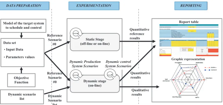
Three consecutive steps compose the proposed benchmarking
process, which are presented inFig. 1.
Thefirst step, calleddata preparation, concerns the sizing and
the parameterization of the case study. Given a generic model of
the target system to schedule and control, thefirst benchmarking
decisionis to choose the“data set”. A data set includes usually an instance of a model of the target system on which the benchmark is applied, accompanied with the input data needed to make this
model work. Once this data set is chosen, the second decision
concerns the definition of the objective function. The couple (data
set, objective function) defines the reference scenario, called
scenario #0. The third decisionto make in this step is to decide
whether or not dynamic behavior should be tested. If yes, then the
fourth and last decisionis that the researchers must decide which dynamic scenarios they are willing to test in a list of dynamic scenarios.
Once defined, scenario #0 contains only static data (i.e., all the
data is known at the initial date), which allows researchers to test deterministic optimization mechanisms for a given set of inputs (e.g., OR approaches, simulation or emergent approaches, multi-agents approaches), especially if only few constraints are relaxed. In this stage, performance measures are purely quantitative. Scenario #0 can be used to test different optimization approaches,
to evaluate the improvement of certain criteria (e.g.,Cmaxvalues),
or to check the basic behavior of a control system in real time where all data are known initially.
The second step, called experimentation, is composed of two
kinds of experiments:
1. Thestatic stage, which concerns the treatment of the reference
scenario (i.e., scenario #0), and
2. The dynamic stage, which concerns the treatment of the
dynamic scenarios.
If the researchers had selected the second option in the previous step, they will execute two types of dynamic scenarios, introducing perturbations (1) on the target system and (2) on the control system itself. In this stage, researchers can test control approaches and algorithms, using the scenario #0 into which some
dynamic events are inserted, which defines several other scenarios
with increasing complexity.
The output of the static stage concerns only quantitative data, while performance measures can be both quantitative (e.g., relative degradation of performance indicators) or qualitative (e.g., robust-ness level) in the dynamic stage. It is important to note that only the static stage is compulsory in the research; the dynamic stage is optional. However, if researchers need to quantify certain dynamic features of their control system, it is necessary for the static stage to be performed before the dynamic stage. Researchers could then design solutions that dissociate or integrate both static and dynamic stages, leading to designing coupling static optimization with
dynamic behavior (e.g, proactive, reactive, predictive–reactive
sche-duling methods, the interested reader can consult Davenport and
Beck (2000), who did a widespread literature survey for scheduling under uncertainty.)
The third step, calledreporting, concerns the reporting of the
experimental results in a standardized way:
– The parameters and the quantitative results from the static and
dynamic stages are summarized in a report table, which facilitates future comparisons and characterization of the approaches, and
– The qualitative results obtained using the dynamic scenarios
are presented via graphic representations.
This benchmark has been generically designed: it can be applied to different target systems, typically production systems, but not only (e.g., healthcare systems). In this paper, this
bench-mark is applied on the flexible job-shop scheduling problem,
whose model is inspired from an existing flexible cell. The
remaining of the paper deals with such an application and is organized according the three introduced steps: data preparation, experimentations and reporting.
3. First step: data preparation
The output of the data preparation step is the reference scenario #0, and if used, the dynamic scenario list to be tested. During this
step, the target system must be defined. According to the method,
this step is decomposed into three stages: the elaboration of the
formal model of the target system, the definition of the data set and
the objective function, all this defining the static scenario #0, and if
used, the elaboration of the dynamic scenario list.
3.1. The formal model of the target system: aflexible job shop system
Since our desire is to ground the benchmark into reality, we propose to get inspiration from a real assembly cell: the AIP-PRIMECA cell at the University of Valenciennes. From an OR perspective, this system can be viewed as Flexible Job Shop, leading to the formulation of a Flexible Job-Shop Scheduling Problem (FJSP). This section presents then the corresponding generic model and a static instantiation of this model to the AIP-PRIMECA cell. The idea is
tofirst formalize a generic FJSP. This formal, highly parameterized
model guarantees a certain level of genericity for future studies or for the development of a parameterized linear program. In a second sub-section, an instantiation of this model is proposed according to the
staticparameters of the AIP-PRIMECA production cell, in other words, all the parameters of the FJSP that will be assumed constant all along this benchmark (e.g., transportation system and its topology, location of machines, standard production times).
3.1.1. Generic model of theflexible job shop scheduling problem
In OR literature, FJSP is considered as a generalization of the traditional job shop problem (JSP). The underlined terms are important to understand the formalization for this benchmark:
Let consider njobs to be processed on different mmachines.
Each jobj has its own production sequence composed of some
elementary manufacturing operations. Those operations or tasks can be executed on one or more machines.
The main difference between FJSP and the JSP is that a machine can perform different types of operations in FJSP. The assignment
of operations to the machines is not a priori fixed like in the
traditional job shop problem. For this reason, many papers used two-phase methods to deal with the FJSP. The assignment problem
is solved in thefirst step, while the second step aims to solve the
sequencing of the assigned operations on machines.
Reference Scenario
#0 Reference
Scenario #0
Static Stage (off-line or on-line)
Dynamic stage (on-line)
Quantitative reference results
Qualitative results Dynamic control System Scenarios Dynamic Production
System Scenarios
Quantitative results
EXPERIMENTATION REPORTING
Report table DATA PREPARATION
Dynamic scenario list Parameters values Data set
Dynamic Scenario
list Objective
Function Input Data
Model of the target system to schedule and control
Most of theflexible job shop problems are proved to be
NP-hard (Conway, Maxwell, & Miller 1967). Theflexibility increase the
complexity of the problem greatly because it requires an addi-tional level of decisions (i.e., the selection of machines on which
job should be proceed) (Brandimarte, 1993). In addition to the
basic constraints (e.g., precedence constraints, disjunctive con-straints), we take into account in our study realistic constraints that are generally omitted. This concerns the transportation between two machines in the production system, the queue
capacity of machines, and jobs limitation in the shopfloor.
In the following, we present a mixed integer linear program (MILP) of the FJSP problem. However, we assume that the behavior is ideal for the best execution of this method (e.g., no machine breakdown is considered; no maintenance tasks are planned).
In order to formulate the FJSP, we introducefirst some
para-meters, variables and the constraints.
Notations for parameters
P set of jobs,P¼{1,2,…,n}
R set of machines,R¼{1,2,…,r}
Ij set of operations of the jobj,Ij¼{1,2,…,|Ij|},j∈P
Oij operationiof the jobj
Rij set of machines that can perform operationOij,Rij∈R
pij processing time of operationi(i∈Ij)
ttr1r2 transportation time from machiner1tor2
MJ maximum simultaneous jobs in the shopfloor
cir input queue capacity of machiner
dj due date of jobj, j¼1,…,n
αj tardiness penalties associated to the jobj, j¼1,…,n
βj earliness penalties associated to the jobj, j¼1,…,n
Notations for variables
tij completion time of operationOij(i∈Ij),tij∈N
μijr a binary variable set to 1 if operationOijis performed on
machiner; 0, otherwise.
bijkl a binary variable set to 1 if operationOij is performed
before operationOkl; 0, otherwise.
trijr1r2 a binary variable set to 1 if job j is transported to
machiner2after performing operationOij; 0, otherwise.
wijr waiting time of operationOijin the queue of machiner
wvijklr a binary variable set to 1 if operationOijis waiting for
operationOklin the queue of machiner; 0, otherwise.
zlj a binary variable set to 1 if jobland jobjare in the shop
floor in the same time; 0, otherwise.
3.1.2. Detail of the constraints
Disjunctive constraints: A machine can process one operation at time, and an operation is performed by only one machine.
tijþpklμklrþBMbijkl≤tklþBM; ∀i;k∈I;∀j;l∈P;∀r∈Rij ð1Þ
whereBMis a large number.
bijklþbklij≤1 ∀i∈Ij;k∈Il;∀j;l∈P ð2Þ
∑ r∈Rij
μijr¼1 ∀i∈Ij;∀j∈P ð3Þ
Precedence constraints:These constraints insure job's produc-tion sequence. The compleproduc-tion time of the next operaproduc-tion con-siders the completion time of the previous one, the waiting time and the transportation time if the two operations are not performed in the same machine.
tðiþ1Þj≥tijþpðiþ1Þjþwðiþ1Þjr2
þ ∑
r1;r2∈R
ttr1r2trijr1r2 ∀i∈Ij;∀j∈P;∀r1;r2∈Rij ð4Þ
∑ r1;r2∈R r1≠r2
trijr1r2≤1; ∀i∈Ij;∀j∈P ð5Þ
Allocation and transportation relationship:If successive opera-tions of a job are performed on different machines, there is a transportation operation between those two machines. Transpor-tation delays are set to zero, and the transporTranspor-tation system has unlimited capacity.
μijr1þμðiþ1Þjr2−1≤trijr1r2 ∀i∈Ij;∀j∈P;∀r1;r2∈Rij;r1≠r2 ð6Þ
μijr1þμðiþ1Þjr2≥ð1þεÞtrijr1r2 ∀i∈Ij;∀j∈P;∀r1;r2∈Rij;r1≠r2 ð7Þ
whereεis a small number.
Queue capacity of the machine input and FIFO rule:Each machine has a limited queue capacity. No more operations than this queue
capacity can wait in the queue. Thefirst job arriving in the queue is
thefirst treated.
bijklþwvijklr≤1 ∀i;k∈I;∀j;l∈P; ∀r∈Rij∩Rkl ð8Þ
bijkl−wvklijr≥0 ∀i∈Ij;∀k∈Il;∀j;l∈P;∀r∈Rij∩Rkl ð9Þ
wvijklrþwvklijr≤1 ∀i∈Ij;∀k∈Il;∀j;l∈P;∀r∈Rij∩Rkl ð10Þ
tij−pijþBMbijklþBMwvklijr≤
tkl−pkl−wklrþ2BM ∀i∈Ij;∀k∈Il;∀j;l∈P;j≠l;∀r∈Rij∩Rkl ð11Þ
wklr≤ ∑ i∈Ij j∈P;j≠l
pijwvklijr ∀k∈Il;∀l∈P;∀r∈Rkl ð12Þ
μijrþμklr≥2ðwvijklrþ wvklijrÞ ∀i∈Ij;∀k∈Ik∀j;l∈P;∀r∈Rij∩Rkl ð13Þ
tijþBMbijkl≤tklþBM ∀i∈Ij;∀k∈Ik;∀j;l∈P ð14Þ
tij−pijμijrþBMbijkl≤tkl−pklμklrþBM ∀i∈Ij;∀k∈Ik;∀j;l∈P;∀r∈R ð15Þ
tij−pijμijr−wijrþBMbijkl≤tkl−pklμklr−wklrþBM ∀i∈Ij;∀k∈Ik;∀j;l∈P;∀r∈R
ð16Þ
∑ l∈P;k∈Il l≠j
wvijklr≤cir−1; ∀i∈Ij;∀j∈P;∀r∈Rij∩Rkl ð17Þ
Limitation of the number of jobs in the system:The number of
simultaneous jobs in the shop floor can be limited by MJ. O0j
defines thefirst operation the jobj(i.e., loading), andOujdefines
the last one (i.e., unloading).
∑ l∈P l≠j
zlj≤MJ−1 ∀j∈P ð18Þ
zjl≥b0lujþb0j0l−1 ∀j;l∈P ð19Þ
zjl≤1−b0l0jþbujul ∀j;l∈P ð20Þ
zjl≥b0l0jþbujul−1 ∀j;l∈P ð21Þ
Variables and constraints in the case of due-date based production
Some constraints and variables must be added only in the case of due-date-based production.
Variables:
Ej: Earliness of job j
Tj: Tardiness of jobj
Constraints:
Ej¼maxfdj−tij;0g ∀i∈Ij;j∈P ð22Þ
Tj¼maxftij–dj;0g ∀i∈Ij;j∈P ð23Þ
Constraints for the type of each variable
tij≥pij ∀i∈Ij;j∈P ð24Þ
bijkl∈f0;1g ∀i∈Ij;j∈P;∀k∈Il;l∈P ð25Þ
trijrr’∈f0;1g ∀i∈Ij;j∈P;∀r;r′∈Rij; ð26Þ
mijr∈f0;1g ∀i∈Ij;j∈P;∀r∈Rij; ð27Þ
3.1.3. Quantitative performance
Different criteria are used in the measurement of the quanti-tative performance. The well-known criteria are cited below, according to the variables and parameters presented above.
Makespanis the time at which the last job is completed. In
general, the makespan is denoted asCmax. Its value is calculated by
the formula
Cmax¼max∀i∈Ij∀j∈Ptij ð28Þ
Flow timeis the time spent by the job in the shop which is equal to the sum of the processing time on each machine, including the process plan for the considered part and the waiting
time in queues. LetCjbe the completion time of the last operation
of the job j. The flow time of the job j is then Cj.
In this case, the objective is to minimize the total completion time:Σ∀j∈PCj
Earliness and tardiness of jobs is the comparison of the actual completion time of jobs with the desired completion time.
The earliness of a jobi isEi¼max(0, di−Ci). In the same way, the
tardiness Ti of a job i is the positive difference between the
completion time and the due date: Ti¼max(0, Ci−di). Different
criteria can be optimized. The goal is to minimize the amount of
earliness (Σ∀i∈PEi), the amount of tardiness (Σ∀i∈PTi) or both criteria
(Σ∀i∈PðαiTiþβiEiÞ or its quadratic form), where αi and βi are
respectively delay cost and handling cost.
Machine utilizationdepends on the shop rather than the jobs. It is a fraction of the machine capacity used in the processing. The
average utilization ofmmachines andnjobs is proportional to the
maximumflow time, as expressed this formula:
U¼Σ∀i∈Ij∀j∈Ppij mCmax
ð29Þ
This criterion is rather a behavioral performance indicator than a production performance indicator, but it is used when bottleneck analysis are performed.
Work in processis the time spend by jobs in the queue before a machine. The objective is to minimize the total waiting time in the
machine inputsW.
W¼ ∑
∀r∈R ∑
∀j∈P ∑
∀i∈Ij
wijr ð30Þ
Multi-objective optimization: The different criteria cited above can be mixed to optimize more than one objective. In the literature, many papers used multi-objective optimization for FJSP (Azardoost & Imanipour, 2011; Ho and Tay, 2008; Taboun and Ulger, 1992), but to the best of our knowledge, no one has taken into account the additional constraints presented in this paper.
3.1.4. Instantiation of the model: application to the AIP-PRIMECA cell
The previous formalization of a FJSP is generic enough to consider its application to the AIP-PRIMECA cell. A short instantia-tion of this model applied to the AIP cell and relevant static parameters are given below. These data are not assumed to change during the static or the dynamic stages.
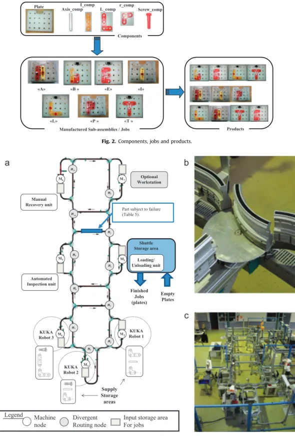
The following data are relative to products.
Components
Six components are available (“Plate”, “Axis_comp”, “I_comp”,
“L_comp”, “r_comp” and “screw_comp”). Purchase orders are
assumed to insure sufficient quantities of these components as
desired. In future research, a limited supply will be considered as a new constraint.
Jobs (Sub-assemblies)
In this paper, seven types of jobs (sub-assemblies) can be manufactured. They are denoted“B”, “E”,“L”, “T”,“A”, “I”and “P”. Components are used to manufacture these types of job.
Production sequence (Ordered manufacturing operations list)
A manufacturing operation is an elementary action carried out on sub-assemblies, which is not a transportation task. There are
eight manufacturing operation types (“Plate loading”,“Axis
mount-ing”,“r_comp mounting”,“I_comp mounting”,“L_comp mounting”,
Screw_comp mounting”,“Inspection”, and “Plate unloading”). For
example,“I_comp mounting”means that the I component must be
mounted on the plate. The inspection is completed by an auto-matic inspection unit (i.e., vision system).
A production sequence (ordered manufacturing operation list) is associated to each type of job. The operation lists have the same structure: a single load, a series of component mountings, a single inspection and a single unloading. Between two successive manufacturing operations, it may be required a transportation operation if the two operations are not done at the same place.
Constraints(6)and(7)ensure this relationship in the MILP.Table 1
shows the different production sequences.
In static scenario, there is no quality issue. In dynamic scenarios, after an inspection, when the job has a quality problem, an extra
manufacturing operation, called “recovery”, must be inserted just
before the plate unloading operation. This is a manual operation that
tries tofix the quality problem. This operation is assumed tofix 100%
of the quality problems.
Table 1
Production sequence for each type of job.
“B” “E” “L” “T” “A” “I” “P”
#1 Plate loading Plate loading Plate loading Plate loading Plate loading Plate loading Plate loading #2 Axis mounting Axis mounting Axis mounting Axis mounting Axis mounting Axis mounting Axis mounting #3 Axis mounting Axis mounting Axis mounting Axis mounting Axis mounting Axis mounting Axis mounting #4 Axis mounting Axis mounting Axis mounting r_comp mounting Axis mounting I_comp mounting r_comp mounting #5 r_comp mounting r_comp mounting I_comp mounting L_comp mounting r_comp mounting Screw_comp monting L_comp mounting #6 r_comp mounting r_comp mounting I_comp mounting Inspection L_comp mounting Inspection Inspection #7 I_comp mounting L_comp mounting Screw_comp mounting Plate unloading I_comp mounting Plate unloading Plate unloading #8 Screw_comp mounting Inspection Screw_comp mounting Screw_comp mounting
#9 Inspection Plate unloading Inspection Inspection
3.1.5. Products, client order
Three kinds of products are proposed to clients. They are called
“BELT” “AIP”and“LATE”. A product is thus a subset of jobs, or
sub-assemblies, among the seven possible job types, corresponding to different arrangements of letters. The jobs that compose these products can be manufactured in any order.
Fig. 2shows pictures of components, jobs and products. The relationships between these elements are highlighted.
A set of different products to complete for a client, possibly with an associated global due date, is called a client order. A product is
consideredfinished when its latest job isfinished and leaves the
cell. In the MILP, this is handled by considering that a client order is as a set of products, and each of these products considered as a set of jobs. Thus, the due date of the client order can be assigned to this whole set of jobs. In other words, each job in the set is
assigned this due date in the MILP (constraints(22)and(23)).
Screw_comp Axis_comp L_comp
I_comp r_comp Plate
Components
Manufactured Sub-assemblies / Jobs
«A» «B » «E» «I»
«L» «P » «T »
Products
Fig. 2.Components, jobs and products.
The following data are relative to machines.
Machines:
The cell is composed of seven machines (Fig. 3a):
– a loading/unloading unit (M1),
– three assembly workstations (M2, M3and M4),
– an automatic inspection unit (M5),
– a recovery unit (M6), which is the only manual workstation in
the cell, and
– an optional workstation (M7), only used for a given dynamic
scenario.
Machines are responsible for the completion of manufacturing operations to do the jobs. Some machines are able to complete the
same manufacturing operation (flexibility, variable μijr, decides
which machine performs which operation in the MILP), while some manufacturing operations can be completed on a single machine.
Supply storage area:
Each assembly workstation has also its own supply storage
area, which is used for supply purpose in components (Fig. 3).
Since, in this benchmark, this supply is assumed infinite, this
supply storage area is not used in the scenarios described in the previous mathematical model.
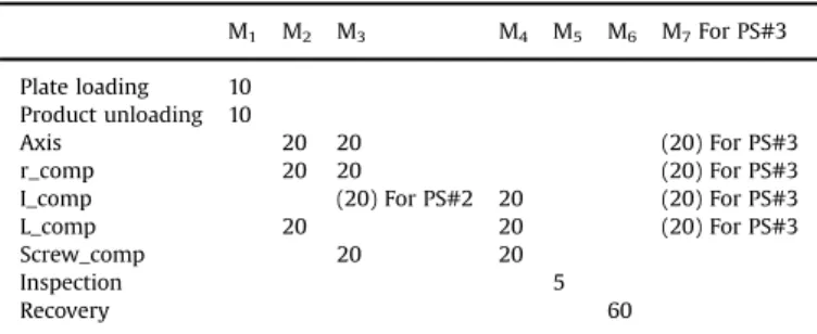
Manufacturing operation processing times:
Table 2 provides the manufacturing operations feasible on the different machines by providing the corresponding manufacturing operation processing times. Otherwise, these machines cannot carry out the manufacturing operations.
The following data are relative to the transportation system.
Topology of the transportation system:
The machines are connected using a transportation system. The transportation system is a one-direction monorail system with
rotating transfer gates at routing nodes (Montech Technology
2009). Thus, this transportation system can be considered as a
directed, strongly-connected graph, composed of the following
nodes (Fig. 3a):
– M1, M2, M3, M4, M5, M6, M7 (white nodes inFig. 3a) are the
machine nodes, and
– n1,n2,n3,n4,n5,n6,n7,n8,n9, n10, n11(gray nodes inFig. 3a) are divergent routing nodes in which routing decisions must be
made (e.g., from n11, it is possible to reach the adjacent nodes
n1or M7).
Fig. 3 gives the whole topology of the cell, including nodes, highlighting the transportation system, the exact machine loca-tion, and the types of components available in its supply storage area.
3.1.6. Shuttles and shuttle storage area
Shuttles are self-propelled transportation resources that
trans-port a job from node to node (Fig. 4a). A maximum of 10 shuttles
are available. At each moment, a maximum of 10 jobs can be
manufactured at the same time (constraints(18)–(21)in the MILP).
Each shuttle embeds a basic behavior to avoid colliding with other shuttles, detect a transfer gate (i.e., stop-and-go system), manage speed in curves and in strait lines, and dock in front of the machines. Because of the technological solution adopted for conveyance, shuttles are governed according to a FIFO rule.
For simplification purposes, it is assumed that empty shuttles
are stored in a specific area near the machine M1, with unlimited
storage capacity. They enter and leave the cell there. Empty shuttles are loaded with the plates (operation #1) when desired
on M1before entering the cell, go to production and then return to
M1where they are unloaded for delivery. Next, they return in this
empty shuttle storage area near M1 until their next use. Thus,
there is no possible empty trip in the cell; in the cell, a shuttle has always a job embedded on it.
3.1.7. Job input storage areas
Before each machine stands a job input storage area with limited capacity, excluding the operating area in front of the
machines (Fig. 4b). This capacity is set in the cell for one shuttle
for all machines (constraint (17) in the MILP). More than one
shuttle in the input storage area is risky since it may lock the transportation system for other products and block transfer gates
by parking on them. Specific rules must be designed to handle this
situation (e.g., shuttles must keep moving in the central loop until a place is free). Despite this, this value can be increased for simulation or theoretical studies, but not for real experimental studies. The transfer time between the job input storage area and the machine corresponds to the time the shuttle has to move from the storage area and to dock in front of the machine. This time is neglected for all the machines.
Table 2
Manufacturing operations processing times (in seconds).
M1 M2 M3 M4 M5 M6 M7For PS#3
Plate loading 10 Product unloading 10
Axis 20 20 (20) For PS#3
r_comp 20 20 (20) For PS#3
I_comp (20) For PS#2 20 (20) For PS#3
L_comp 20 20 (20) For PS#3
Screw_comp 20 20
Inspection 5
Recovery 60
Note: Some values in this table have been modified recently in dynamic scenarios that focus on perturbations applied to the production system (i.e., dynamic scenarios PS#2 and PS#3). The corresponding cells are light gray with data between parentheses.
3.1.8. Theoretical transportation times
Table 3 shows the theoretical transportation time that is associated to each couple of adjacent nodes. This time is called theoretical since it depends on the actual speed of shuttles. In fact,
in reality, a transportation process may last longer that this time due to unexpected events or jamming phenomena.
3.2. The data set and the objective function
Given a formal generic model of the targetflexible job-shop
system, this section tries to define the reference scenario #0 to be
chosen by the researchers for the whole benchmark. In this scenario, all the data is known initially. In other words, there are no perturbations. In scenario #0, there is no quality problem, and
100% of the jobs pass inspection. Thus, machine M6(i.e., recovery)
must never be used in the static scenarios.
To design the scenario #0, the researchers must choose a data
set,fixing two parameters: (1) the set of client orders, eventually
with due dates, and (2) the constraints to be handled. In addition to this data set, the objective function, or performance function,
must be determined.Table 4presents the proposed different data
sets. Data sets, in which the constraints are relaxed (e.g., infinite
number of shuttles and/or infinite storage capacity and/or
neglected transportation times), can be used to obtain bounds or to test basic optimization mechanisms. If the number of shuttles is
assumed infinite, then constraints (18)–(21) in MILP should be
relaxed. If the input storage capacity is assumed infinite, then it is
constraint(17)that needs to be relaxed. Finally, if transportation
times are neglected, then constraints (6) and (7) need to be
relaxed. If a due-date-based strategy is chosen, the objective function will be different from the makespan; thus, constraints
(22)and(23)should be considered in this case.
For researchers who pay attention to due-date based produc-tion, desired due dates for client orders are provided in the last
column ofTable 4. These dates have beenfine-tuned according to
the possible constraint relaxation that may lead to shorten production delays. The problem to be solved has to provide an
accurate value for these due dates. As Gordon, Proth, and Chu
(2002) noted, there are quite few results on flow and job shop with due-date assignment, and most of the papers are on single and parallel machine shops. Most studies on due-date based scheduling assume uniform distribution of due dates. However, in real production system, this assumption does not always hold true(Thiagarajan and Rajendran, 2005).Sourd (2005)presented a
different method for generating due dates that defines the interval
bounds in which due dates belong. Those bounds, or range factors, try to control the tightness and variance of due dates. This
Table 3
Theoretical transportation times between adjacent nodes (in seconds).
Destination nodes
Source nodes N1 N2 N3 N4 N5 N6 N7 N8 N9 N10 N11 M1 M2 M3 M4 M5 M6 M7
N1 4 – – – – – – – 5 – – – – – – – –
N2 – 4 – – – – – – – – 5 – – – – –– –
N3 – – 4 – – – 5 – – – – – – – – – –
N4 – – – 4 – – – – – – – 5 – – – – –
N5 – – – – 3 – – – – – – – 11 – – – –
N6 – – – – – 4 – – – – – – – 5 – – –
N7 – – – 5 – – 4 – – – – – – – – – –
N8 – – – – – – – 4 – – – – – – 5 – –
N9 – 5 – – – – – – 4 – – – – – – – –
N10 – – – – – – – – – 4 – – – – – 7 –
N11 9 – – – – – – – – – – – – – –– – 10
M1 – – – 6 – – – 7 – – – – – – – – –
M2 – – – – – 5 – – – – – – 13 – – – –
M3 – – – – – – 6 – – – – – – 7 – – –
M4 – – – 7 – – – 6 – – – – – – – – –
M5 – 7 – – – – – – – 6 – – – – – – –
M6 12 – – – – – – – – – – – – – – – 13
M7 – 6 – – – – – – – 7 – – – – – – –
Table 4
Description of the possible data sets to design scenario #0.
Client order
Number of shuttles
Input storage capacity
Transportation times
Order #
Products Due date (s) (if pull/JIT mode, else not used) BELT AIP LATE
A0 Infinite Infinite Zero #1 1 – – 325
#2 – 1 – 209
B0 10 1 Table 3 #1 – 2 – 327
C0 4 1 Table 3 #1 1 – – 382
#2 – 1 – 238
D0 Infinite 1 Zero #1 1 – – 321
#2 2 1 – 863
E0 Infinite Infinite Table 3 #1 2 1 – 947
#2 – 2 1 786
#3 – – 2 637
F0 Infinite 1 Table 3 #1 – 1 3 961
#2 2 1 – 880
#3 1 1 1 919
G0 8 Infinite Zero #1 1 2 1 1032
#2 2 3 1 1409
#3 3 2 3 2480
H0 10 Infinite Table 3 #1 1 2 1 992
#2 2 3 1 1676
#3 3 2 3 1801
I0 10 1 Zero #1 2 2 3 1709
#2 2 4 – 1356
#3 3 2 3 2276
J0 10 1 Table 3 #1 4 4 4 2793
#2 6 5 1 3175
#3 – 8 3 2266
K0 10 1 Table 3 #1 8 10 12 9067
#2 10 8 10 7342
#3 12 10 8 6841
L0 10 1 Table 3 #1 15 20 25 17122
technique was used by many other authors, for example,Cho and Lazaro (2010).
For instance, let consider two parameters: the average
tardi-ness factorτand the range factorρ. Due dates are thus generated
from the uniform distribution:
max 0;ð1−τ−ρ=2Þðddoþ ∑
j∈J;i∈Ij pijÞ
!
;ð1−τþρ=2Þðddoþ ∑ j∈J;i∈Ij
pijÞ
" #
ð31Þ
where ddo is the minimum transportation time to perform the
client-ordero. When the transportation time is neglected,ddois
set to 0.τandρcan take different values in the sets:τ∈{0,2; 0,4;
0,6; 0,8}, ρ∈{0; 0,2; 0,4; 0,6;0,8}. The due dates in Table 4 are
generated for τ¼0.2 and ρ¼0.5, and values are rounded to the
nearest integer.
Obviously, the model's objective function that takes into
account due dates must logically take into consideration tardiness or earliness of products. For researchers who do not pay attention to due dates, these dates can be ignored, and other traditional
criteria (e.g.,Cmax) can be used. At the designer's discretion, new
scenario can be designed, and a combination of these quantitative indicators or a multicriteria analysis can be performed.
3.3. The dynamic scenario list
If testing the dynamic scenarios, several dynamic scenarios must be chosen to evaluate the control system in case of
unexpected events.Tables 5and6give a list of dynamic scenarios,
numbered according to the increasing complexity level. InTable 5,
dynamic scenarios concern the perturbation of the production
system; Table 6 provides the dynamic scenarios related to the
perturbation of the control system itself. Obviously, researchers can introduce new scenarios or use these scenarios with different parameters. Otherwise, this list can be considered as a reference list for future comparisons.
For all these scenarios, when a resource (i.e., machine or
conveyor) becomes unavailable, the jobs that are in the resource's
waiting queue are able to leave, if desired. Thus, they do not stay blocked at this resource and can be reallocated elsewhere.
4. Second step: experimentation
In the experimentation step, the production control system or
model is tested under the conditions defined in the reference
scenario, possibly with a list of dynamic scenarios.
4.1. Static stage
In the static stage, the control system is running under the
reference scenario #0, and the experimental results, reflecting
the system performance, are collected. These results describe the observed performance level (e.g., throughput rate or machine utilization rate) that make it possible to analyze the system performance and to compare the performance of different sys-tems; however, they do not tell why the performance is as it is. These results cannot reveal which factors account for differences in different measured performance levels.
In this stage, the experiment considers static data (i.e., perturba-tions are not considered) that lead to quantitative performance indicators, which are based on statistical theory. These quantitative
performance indicators defined in the benchmarking framework
have been previously introduced (e.g., makespan, throughput).
The static stage can be performedoff-line, allowing, for
exam-ple, optimization mechanisms before the real or simulated on-line
applications. Usually, real-time constraints are not considered in
such off-line approaches, and very efficient optimization tools,
typically metaheuristics, can be designed. This stage can also be
performedon-line–in other words,“on thefly”or in real time–
applied to the real cell or a real-time simulator/emulator of the cell. The difference between the off-line and on-line experimenta-tion is that the time to construct the scheduling plan may impact the results if the experimentation are on-line. However, this remains a static stage in that all the input data used to construct the scheduling plan are deterministically known at the initial date.
4.2. Dynamic stage
In the dynamic stage, certain data are not known at the initial
time, usually perturbations. If the benchmark's dynamic feature is
dealt with, for each dynamic scenario to be tested, the researchers always compare scenario #0: the reference scenario. Thus, the same conditions (i.e., data set and objective function) chosen for scenario #0 must be applied to allow a coherent relative compar-ison. In addition, the same models and algorithms as the ones proposed by the researchers for the static stage must be used for a coherent analysis.
These scenarios must be logically considered on-line: the real or simulated production system continues to evolve, and faced with unpredicted events, the control system must react. If the control system takes too much time (simulated or real time) to react, it must affect the production and degrade the performance. Dynamic algorithms and simulation must be extensively used by researchers. Obviously, the control system must not know about the perturbations before they occur.
In dynamic environments, performance is harder to evaluate than in static environments. We can identify two ways to perform this performance evaluation:
Quantitative: Since scenario #1 and the following scenarios (Tables 5and6) are all based upon scenario #0, it is possible to evaluate the performance deterioration by comparing the evolution of quantitative indicators (e.g., percentage increaseof theCmaxvalues faced with a breakdown).
Qualitative: Quantitative indicators may not be sufficient from a control perspective, whereas other more qualitative criteria should be analyzed: robustness and/or reactivity. These quali-tative indicators are more subjective. They cannot be directly obtained from the experimental data, but they can be esti-mated. Since several different scenarios in dynamic situationshave been proposed, it would be possible to define a
lexico-graphical notations based upon the class of dynamic scenario effectively supported by the candidate control system.
In terms of qualitative performance indicators, this benchmark focuses on the robustness parameter, which is the ability of a control system to remain working correctly and relatively stable, even in presence of perturbations. Ideally, measuring robustness requires analyzing the system with all possible natural errors that
can occur, which is not possible in reality. Verifying the system's
operation and waiting for the occurrence of errors that occur infrequently is too time consuming. Until now, there has been no effective approach to quantitatively measure the robustness of a manufacturing control system. This benchmark considers the set
of dynamic scenario tests, defined inTables 5 and6, to verify if
the control system remains working correctly after the perturba-tion occurs. The evaluaperturba-tion of the qualitative aspect is based on
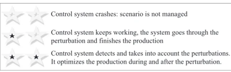
notation using stars (Fig. 5). A number of stars (0, 1 or 2) is
Table 5
Dynamic production system scenarios.
Scenario Description Highlighted control behavior Parameters
#PS1 All orders are canceled before production. This scenario simulates a capacity to cancel orders and wait for a full restart
Machines: all Start time: date 0
#PS2 At a given time, one of the machines was improved and is now able to perform a new kind of manufacturing operation, which increases the
flexibility level of the cell.
This scenario simulates a technological evolution forwarded in a production system.
The evaluated control capacity is the capacity of the control system to adapt to evolution of machines.
Machine: M3 Operation: I_comp
Start time: just after the departure of the second shuttle from M3
Updated processing time: 20 s.
(seeTable 2, Manufacturing Processing Times)
#PS3 At a given time, a new machine is added to the manufacturing cell and is immediately available for production.
This scenario simulates that machines are sometimes under maintenance for a long time and cannot be available.
The evaluated control capacity is the capacity of the control system to adapt to evolution of the cell topology.
Machine: M7
Operations available: Axis_comp, R_comp, I_comp and L_comp
Start Time: just after the departure of thefirst shuttle from M2.
New processing times: seeTable 2, last column, Manufacturing Processing Times.
#PS4 At a given time, the machine processing time increases for all its operations in a given time window.
This scenario simulates the wear of a tool that is replaced (i.e., maintenance).
The evaluated control capacity is the capacity of the control system to adapt to evolution of the machine processing time.
Machine: M2
New processing time: 40 s
Start Time: just after the departure of the second shuttle from M2.
Duration (seconds): 25Total number of jobs
If a job is processed by M2, when the processing time returns to 20 s, the 40-s processing time is used for the current operation.
#PS5 At a given time, a rush order appear. This scenario simulates the fact that client desires may evolve over time.
The evaluated control capacity is the capacity of the control system to manage the introduction of a rush order.
Type of order: AIP
Arrival Time: just after the end of the production of the fourth job in the cell. Due date: ASAP
#PS6 After a quality control, a product is canceled. This scenario simulates the fact that product may not satisfy the client.
The evaluated control capacity is the capacity of the control system to manage product cancellation.
Product canceled: BELT
Date: just after the inspection of thefirst job of a BELT product.
#PS7 At a given time, a part of the conveyor system is due for maintenance in a given time window.
This scenario simulates that the conveying system has a limited reliability.
The evaluated control capacity is the capacity of the control system to manage a routing change.
Start time: just after the fourth job is unloaded. The conveyor must no longer accept shuttles, and as soon as it is empty, the maintenance starts.
Location of the part: part between nodes n9 and n2located onFig. 3a
Duration (seconds): 25Total number of jobs
#PS8 After a number of components mounted with a certain machine, the component is lacking in a given time window.
This scenario simulates that supplies are always limited and must be adjusted.The evaluated control capacity is the capacity of the control system to manage stock re-provisioning.
Type of Component: Axis_comp Machine: M3
Number of mounted components before being lacking: 10
Duration (seconds): 25Total number of jobs.
#PS9 At a given time, one of the redundant machines will go down in a given time window.
This scenario simulates that the machines have a limited reliability.
The evaluated control capacity is the capacity of the control system to manage a redundant machine's breakdown.
Machine: M2
Start time: just after the departure of thefirst shuttle from M2.
Duration (seconds): 25Total number of jobs
#PS10 At a given time, one of the critical machines (i.e., the only one that can perform a given task) will go down in a given time window.
This scenario simulates that a critical machine may result in the breakdown of the whole production system.
The evaluated control capacity is the capacity of the control system to manage a critical machine's breakdown.
Machine: M4
Start time: just after the departure of the second shuttle from M4.
Duration (seconds): 25Total number of jobs.
#PS11 A quality problem is added to the production system, and the recovery M6workstation must be used each time the inspection detects a quality problem.
This scenario simulates that quality issues are sometimes discovered during the production and must be solved on-line.
The evaluated control capacity is the capacity of the control system to manage products that have defects.
Three steps are defined: (1) star awarding system, (2) qualitative scoring of robustness, and (3) quantitative scoring of robustness.
4.2.1. Star awarding system
Fig. 5 proposes the star awarding system, which is given for each dynamic scenario tested.
Table 7summarizes the overall criteria for the 0 and 2 star rates for each of the dynamic scenarios. The one between these two limits would be rated with 1 star, since they could have displayed better behavior.
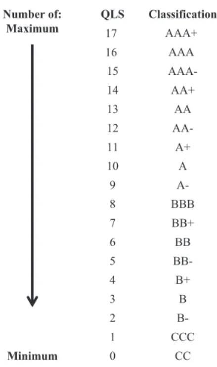
4.2.2. Qualitative scoring of robustness
The final qualitative classification depends of the number of
stars that each approach obtains. To generalize this classification
method, balancing the number of 2-star and 1-star ratings, researchers are invited to use the QuaLitative Score (QLS) formula:
Q LS¼max 2n ;1
21
n
ð32Þ
This means that the researchers must select the row that maximizes the number of 2-star ratings and half of the 1-star
ratings. This choice is justified by the maximum number of higher
classification must be ranked better. For example, an approach that
obtains 5 times a 2-star rating and 6 times a 1-star rating, the
researchers must select the row 5, sinceQLS¼max(5, 0.56)¼5.
Thus, to obtain the maximum rating, the approach gives all the
Table 6
Dynamic control system scenarios.
Scenario Description Highlighted control behavior Parameters
#CS1 At a given time, a decisional entity breaks down for a pre-determined amount of time.
This scenario simulates that hardware supporting decisional functions have a limited reliability in a centralized or distributed architecture.
The evaluated control capacity is the capacity of the control system to manage the loss of one of its decisional entities.
Targeted decisional entity: in centralized architecture, the computer supports the whole control process. In distributed architecture, the entity is selected randomly among the set of decisional entities (e.g., jobs, machines). Start Time: : just after the end of the third job Duration (seconds): 25Total number of jobs
#CS2 At a given time, the network supporting the communication among decisional entities breaks down for a pre-determined amount of time.
This scenario simulates that network communication may be a constraint in a distributed architecture.
The evaluated control capacity is the capacity of the control system to manage the loss of the decisional network.
Start Time: just after the end of the third job Duration (seconds): 25Total number of jobs Table 5(continued)
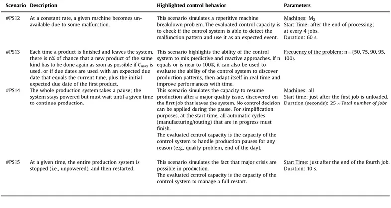
Scenario Description Highlighted control behavior Parameters
#PS12 At a constant rate, a given machine becomes un-available due to some malfunction.
This scenario simulates a repetitive machine breakdown problem. The evaluated control capacity is to check if the control system is able to detect the malfunction pattern and use it as an expected event.
Machines: M2
Start Time: after the end of processing; at every 4 jobs.
Duration: 60 s.
#PS13 Each time a product isfinished and leaves the system, there is n% of chance that a new product of the same kind has to be done again as soon as possible ifCmaxis used, or if due dates are used, with an expected due date that equals the current time, plus the initial expected due date of thefirst product.
This scenario highlights the ability of the control system to mix predictive and reactive approaches. If n equals or is near to 100%, it can also be used to evaluate the ability of the control system to discover production patterns, then adapt itself in real time and improve performances with time.
Frequency of the problem: n¼{50, 75, 90, 95, 100}.
#PS14 The whole production system takes a pause; the system stays powered but must wait until a given time to continue production.
This scenario simulates the capacity to resume production after a major quality issue, discovered on thefirst job that leaves the system. No control decision can be applied during the pause. For simplification purposes, at the start time, all automatic cycles (manufacturing/routing) that are in progress must
finish.
The evaluated control capacity is the capacity of the control system to handle production pauses for any reason (e.g., quality problem, end of the day).
Machines: all
Start time: just after thefirst job is unloaded. Duration (seconds): 25Total number of jobs
#PS15 At a given time, the entire production system is stopped (i.e., unpowered), and then restarted.
This scenario simulates the fact that major crisis are possible in production.
The evaluated control capacity is the capacity of the control system to manage a full restart.
dynamic scenarios with the maximum 2-star score, as given by:
QLS¼max(17, 0.50)¼17. Fig. 6 presents the different ratings
obtained and the name of each classification.
Of course, this rating should be only used if at least one dynamic scenario is performed.
4.2.3. Quantitative scoring of robustness
The qualitative scoring does not allow researchers to compare the quality of the control system. It only states how well the control system handles the dynamic scenario (i.e., well: 2 stars, average: 1 star, or poorly: 0 star). This study can be completed to quantify to what degree the handling is effective. For example, if two control systems faced with the same dynamic scenario are rated with 2 stars, the resulting deteriorated makespan can be higher for one than the other. The degree of robustness is
quantified in this step. This quantification is based on the results
obtained with the dynamic scenarios weighted by the perfor-mance deterioration and evaluated with the reference scenario #0.
This quantification also takes into account whether or not the
objective function minimized or maximized.
If a minimized objective function is the goal, the QuanTitative Score (QTS) formula must be used:
Q TS¼ ∑ 0oi≤15
gi
eðOpref−Opi=OprefÞ;ifOp i4Opref 1;otherwise
( !
eðOpbest−Opi=OpbestÞ;ifOp i4Opbest 1;otherwise
( !
ð33Þ
If a maximized objective function is the goal, the following formula must be used:
Q TS¼ ∑
0oi≤15
gi
ðOpi=OprefÞ;ifOpioOpref
1;otherwise
( !
n
ðOpi=OpbestÞ;ifOpioOpbest
1;otherwise
( !
ð34Þ
wheregiis the grade of scenarioi(0, 1 or 2 stars);Oprefis the value
obtained in the optimization criteria in the reference scenario;
Opi is the value obtained in the optimization criteria in the
dynamic scenarioi; andOpbestis the overall best result obtained
for the reference scenario #0. With this formula, the best overall score is 30 but is unreachable. It corresponds to the situation in which the control system is awarded with 2 stars for each dynamic scenario, no performance deterioration occurs in all these scenar-ios, and the result for the reference scenario #0 is the best one.
Evaluating the robustness of a control system in the dynamic stage is not simple and is a hard research problem in itself. Our evaluation method can be discussed and improved, especially if the quantitative score requires the best solution (i.e., the optimal
one). It has the advantage to be a first evaluation method for
robustness, and researchers are encouraged to use it and improve it. This can open up new interesting research areas. Of course, this evaluation can be skipped by researchers using this benchmark or can be stopped at the second step.
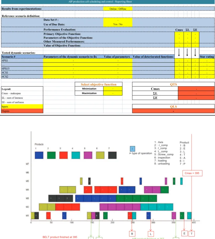
5. Third step: reporting
When the experimental results are available, it is important to present them explicitly. First of all, for each scenario (scenario #0
and dynamic scenarios), a Gantt diagram (e.g., Gantt machine) can be provided for graphic representation and intuitive behavioral analysis of our approach. However, this is not enough. A clear reporting of the results would help the researchers to understand the inputs and outputs of the benchmark when designing their models, forcing them to use a common method to summarize and standardize their results. This would facilitate the objectives for future comparisons between different approaches when other researchers publish their results. In that direction, we propose a reporting sheet to summarize the information related to the selected static and dynamic scenarios, design choices and
perfor-mance indicators.Table 8gives an example of such a sheet.
Finally, a conclusion must be proposed to point out the main features of the proposed approach, the lessons learned and the
proposal's limits.
6. Three illustrative applications
To facilitate the appropriation of this benchmark, three
differ-ent applications are presdiffer-ented consecutively. The first uses the
benchmark through a mixed-integer linear program. In the two
other applications, the same potential fields control approach is
the focus, in simulation (second application) and in real experi-ments (third application). For each application, the benchmarking process is strictly applied, and the three steps (i.e., data prepara-tion, experimentation and reporting) are given in detail.
These applications do not consider complex data sets since they are provided just for illustration purpose. Designing complete, exhaustive studies using the benchmark is beyond the scope of this paper. Meanwhile, the variety from the three proposed applica-tions enable to show how this benchmark can be used with an OR
approach (first application) or a control approach (second and third
applications), and for the control approach, both in simulation (second application) and in a real system (third application). Of course, full, in-depth studies will be led in the near future, featuring
innovative scientific approaches.
6.1. Using the benchmark through a linear program
The benchmark's formal model of the Mixed-Integer Linear
Program (MILP) was implemented using Cplex.2. The Cplex
solu-tion is based on branch-and-cut algorithm and other OR techni-ques implemented by IBM ILOG. The main idea of these technitechni-ques
is to subdivide the whole problem into sub-problems by fixing
variables at each iteration. A search tree is built and explored to meet the optimal solution. At each node of the tree, a lower bound and an upper bound is computed. If Cplex is stopped before
finding an optimal solution, the best feasible solution is considered
as an upper bound.
Solving the MILP leads to an off-line solution that takes into account the whole list of constraints. The complexity of the model depends on the number of constraints and variables, especially the integer ones. In our case, the number of constraints and variables are very important, and some of them are binary, which make solving the problem very hard.
6.1.1. Data preparation
The chosen data set is C0 (seeTable 4). It is composed of two
client orders: (1) one product, BELT and (2) one product, AIP. The
objective function chosen is the makespan (i.e., Cmax), thus due
dates are not considered. Using a linear program or another OR
Control system crashes: scenario is not managed
Control system keeps working, the system goes through the perturbation and finishes the production
Control system detects and takes into account the perturbations. It optimizes the production during and after the perturbation.
Fig. 5.Star awarding system.
approach requiresa prioriknowledge of the whole system beha-vior. However, if a dynamic scenario is chosen, these approaches are hardly suitable if unexpected events occur.
Thus, no dynamic stage is tested in our study,Liu, Ong, and Ng
(2005), Fattahi and Fallahi (2010) and Adibi, Zandieh, and Amiri (2010)can be cited to justify this choice. These authors'approaches are based on pure adaption of the OR methods to the dynamic
behavior or on hybridization with artificial intelligence, such as agent
systems. The picture of the solution can be taken when the
unexpected event occurs and then the non-finished tasks can be
rescheduled, taking into account the new behavior (Huang, Lau, Mak,
& Liang 2005).
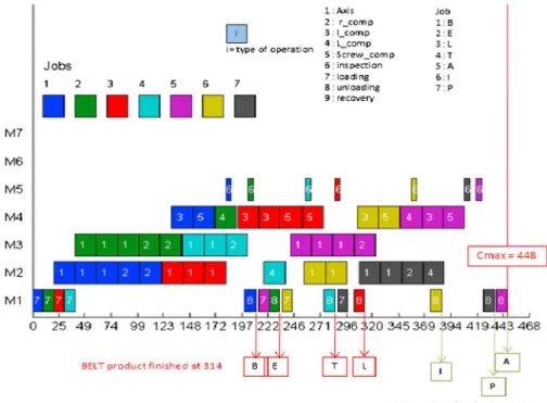
6.1.2. Experimentation
The linear programming technique used in Cplex gives an
off-line solution for the static stage.Fig. 7presents a GANTT diagram
for scenario #0.
The allocation of operations is well-balanced on different
machines, with a little overloading of the machine M3. This
overload is due to the decision of allocating the jobs B, E and P that require many operations of type 1 (Axis) and type 2 (r_comp). Successive Axis and r_comp operations are performed in the same
machine when possible. Choosing machine M3 instead of M2 in
some cases can be explained by the fact that the machine M2is not
able to perform the L_comp operations, so it is discharged. The makespan obtained with Cplex is the optimal one. It will be used for the robustness evaluation of both simulations and experiments proposed in the rest of this paper.
As previously written in the preparation step, the dynamic stage is not dealt with the MILP program presented above. The resolution time of the MILP for this simple case is long (i.e., more than 1 h). If a perturbation occurs the model has to be re-parameterized and solved again by the MILP. Thus, in a dynamic context, this kind of approach cannot be considered without releasing some constraints, which must be carefully studied otherwise. In a dynamic context, this clearly militates to design for example effective meta-heuristics approaches or more reactive control systems, which is currently under development in our team.
6.1.3. Reporting
Table 9 presents the reporting sheet that summarizes this experiment; it only considers the static scenario.
6.2. Using the benchmark through simulation
In this section, a simulation tool based on potential fields is
proposed for the scheduling and the control of the applied
AIP-PRIMECA flexible job-shop. According to the potential field
approach, the machines emit attractive fields to attract the
shuttles (i.e., jobs) depending on the services they provide, their
Table 7
Star rating of the dynamic scenarios.
#PS1 Scenario is not managed or orders cannot be canceled or restarted.
Orders are canceled. The control system checks the orders to detect possible changes and restarts them.
#PS2 Scenario is not managed or the control system crashes. The control system detects the new operation and re-optimizes its production with it. #PS3 Scenario is not managed or the control system crashes. The control system detects the new machine and re-optimizes its production with it. #PS4 Scenario is not managed or the control system crashes. The control system detects the new time and re-optimizes its production with it. #PS5 Scenario is not managed or the control system crashes. The control system detects the rush order and minimizes its completion time. #PS6 Scenario is not managed or the control system crashes. The control system detects the faulty products and makes them rapidly quit the cell. #PS7 Scenario is not managed or the control system crashes. The control system detects maintenance and products are rerouted.
#PS8 Scenario is not managed or the control system crashes. The control system detects the component out of stock and reallocates the products. #PS9 Scenario is not managed or the control system crashes. The control system detects the breakdown and reallocates products to other machines. #PS10 Scenario is not managed or the control system crashes. The control system detects the breakdown and products are changed or are in a waiting
zone.
#PS11 Scenario is not managed or the control system crashes. The control system detects the defect and re-optimizes the products at the manual station. #PS12 Scenario is not managed or the control system crashes. The control system detects the pattern and uses it at expected event.
#PS13 Scenario is not managed or the control system crashes. The control system detects the pattern and uses it at expected event.
#PS14 Scenario is not managed or the control system crashes. The control system checks the state of all the entities and restarts them in their previous state.
#PS15 Scenario is not managed or the control system crashes. The control system checks the state of all the entities and restarts them in their previous state.
#CS1 The control system is totally crashed and is not able to recover. The control system is able to see the missing entity, adapts itself by re-optimizing the plan, recovers and can fulfill all of its plans
#CS2 The control system is not able to start over when the communication network becomes available.
The system continues the normal functioning and adjusts its plans, when the communication network becomes available.
Number of: Maximum
QLS Classification 17 AAA+
16 AAA
15
AAA-14 AA+
13 AA
12
AA-11 A+
10 A
9
A-8 BBB
7 BB+
6 BB
5
BB-4 B+
3 B
2
B-1 CCC
Minimum 0 CC
queue and their real-time availability. To take transportation
times into account, these fields are modified for the distance in
which they are sensitive. Shuttles sense thefields through the cell
at each node and move to the most attractive one until they reach a service node, and the decisions are made on routing divergent node. Thus, if several machines emit concurrent
fields, the shuttle's choice is reduced to the comparison between
the differentfields, which is a very simple‘max’operation. (For
more details on the conceptual and application components,
interested readers can consultZbib, Pach, Sallez, and Trentesaux
(2012).
Since the potentialfield approach is naturally distributed, with
no centralized information storage or information processing, the
NetLogo multi-agent environment (Wilensky, 1999) was used for
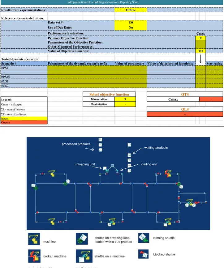
Table 8
Example of a reporting sheet.
Results from experimentations:
Reference scenario definition:
Tested dynamic scenarios:
Scenario # Value of parameters Value of deteriorated functions: Star rating
Legend:
Select objective function
Data Set # : Use of Due Date:
Performance Evaluation: Primary Objective Function: Parameters of the Objective Function: Other Measured Performances: Value of Objective Function:
Parameters of the dynamic scenario to fix
Cmax
Cmax
-QTS
QLS
1 : Axis 2 : r_comp 3 : I_comp 4 : L_comp 5 : Screw_comp 6 : inspection 7 : loading 8 : unloading i
i= type of operation
Product 1 : B 2 : E 3 : L 4 : T 5 : A 6 : I 7 : P
B L E T
I P A
BELT product finished at 395
AIP product finished at 357
Cmax = 395