M
ASTER OF
S
CIENCE IN
A
CTUARIAL
S
CIENCE
M
ASTERS
F
INAL
W
ORK
I
NTERSHIP
R
EPORT
T
AYLOR
F
RY
C
ONSULTING
A
CTUARIES
B
RAM
K
IERKELS
M
ASTER OF
S
CIENCE IN
A
CTUARIAL
S
CIENCE
M
ASTERS
F
INAL
W
ORK
I
NTERNSHIP
R
EPORT
T
AYLOR
F
RY
C
ONSULTING
A
CTUARIES
B
RAM
K
IERKELS
SUPERVISOR(S):
Contents
1 Introduction 3
2 Properties of workers’ compensation self-insurers 5
3 Economic Assumptions 7
3.1 Inflation Rate . . . 7
3.2 Discount rates . . . 13
3.3 Superimposed Inflation . . . 23
3.4 Expense Rate . . . 23
4 Grossing up the Data 24 5 Projected Number of claims 26 6 Valuation Methods 28 6.1 Chain Ladder Method . . . 28
6.2 PPCI Method . . . 29
6.3 PPCF method . . . 30
6.4 ICD method . . . 31
6.5 PCE method . . . 33
6.6 BF method . . . 35
6.7 Results . . . 39
1
Introduction
As the final part of the master degree, I started my internship on 25
Febru-ary 2013 at Taylor Fry Consulting Actuaries. During the internship my work
mainly involved analyzing the outstanding workers’ compensation liabilities
for self-insured clients. In this report I will describe the process of this
anal-ysis.
Workers’ compensation insurance covers employees’ medical expenses, a part
of their lost wages in case of injury or disease and legal costs made to pursue
a claim. A benefit can also be paid to relatives of a worker who’s killed on
the job. The employer is mandated to have workers’ compensation insurance.
The employer can either rely on an insurer or he may opt to self-insure. The
latter means the company is responsible for their own claims management. In
order for a company to be able to manage their own risk, predict the number
and severity of future claims, a company needs a large historical data set with
a significant number of claims. This is the reason small companies rely on an
insurer whereas larger companies, with say 5000 employees or more choose
to self-insure. A company choosing to self-insure envisages that the overall
cost of retaining their financial risk is cheaper than to purchase insurance
from a commercial insurance company. Another reason that self-insuring, to
the utmost extent, only works for larger companies is that claims have to be
paid as they are received, meaning the company requires to have a cash-flow
elects to self-insure it has to decide whether to manage their risk internally
or to outsource the job to a third party.
Throughout this report I will explain the procedures I used to value
out-standing claims. I will use examples based on one particular client, referred
to as ”ABC”. ABC has chosen to outsource the job to Taylor Fry and has
provided us with data containing all claims and transactions between the 1st
of January 2000 and 31st of April 2013. The valuation is to be undertaken
2
Properties of workers’ compensation
self-insurers
Workers’ compensation is a typical long-tailed line of insurance. This means
the majority of claims incurred in a year remain open after, say 3-5 years.
Workers’ compensation claims are further characterized by a large delay
(sev-eral years) between the event leading to an insured loss and the notification
of the claim. Another feature is the long handling period (open claim) in
which payments to cover, for example, medical expenses, legal costs, and
loss of wages are made. Also, workers’ compensation claims have a
signifi-cant frequency of reopened claims; this happens for instance when the health
of the claimant has deteriorated beyond the stage that was the basis of the
original compensation.
ABC provides us with a dataset containing all claims and transactions. If
we denote accident quarters by i then for accident quarter i the number of claims reported with delay d is Nid, for i = 1, . . . , I and d = 0, . . . , I −1,
whereI is the current period. The total payment for the corresponding acci-dent quarter with delay d is denoted by Yid. This payment Yid is the sum of
individual claim amounts or severities {Yid(k) : k = 1, . . . , Nid}. Every claim
that occur at different times t = 0, . . . , T. So a single claim
Yid(k) =
T
X
t=0
Uidt(k). (1)
The last transaction will occur at timeT, as long as the claim remains open we don’t know which future point in time corresponds to T.
Together with the dataset containing all claims and transactions ABC
pro-vides us with a file containing all open claims and their case estimates. The
case estimate Vid(k), determined by the claim handler, reflects his estimation of what the ultimate cost of the claim will be. For an open claim the
to-tal estimated claim costs or the incurred cost Wid(k) is the sum of the past transactions and the case estimate. If T0 is the current time then
Wid(k) = X
tT0
Uidt(k)+Vid(k). (2)
The case estimate can change over time due to new information on the
indi-vidual claim or other similar claims.
An appointed analyst will use the received data and an analytical software
program (SAS) to output triangles containing the number of claims reported,
gross payments and case estimates for each accident and development month,
quarter or year. It is customary to separate the data into large and non-large
removing them ensures that they don’t bias the assessment of the remaining
bulk of the claims. Aside from a few large claims, there may be other causes
that have the potential to distort the analysis undertaken. A large number
of small claims could in fact be related to the same common event and
there-fore their outcomes are not independent. For example asbestos and other
potential claims, where individual claims are not large but instead all relate
to the same source of underlying exposure.
If the accident dates go far back in time it is customary to group the data
be-fore a predetermined date. In our example of ABC we will group the results
prior to 1995.
3
Economic Assumptions
Throughout the analysis we use four economic variables namely; the inflation
rate, the discount rate, superimposed inflation and the expense rate.
3.1
Inflation Rate
The inflation assumption is based on the Access Economics March 2013
fore-casts for the Consumer Price Index (CPI), the Labour Price Index (LPI) or
the average weekly earnings (AWE). The Consumer Price Index (CPI)
mea-sures quarterly changes in the price of a ’basket’ of goods and services which
account for a high proportion of expenditure by the CPI population group.
ser-vices resulting from market forces. The LPI is unaffected by changes in the
quality or quantity of work performed, that is, it is unaffected by changes in
the composition of the labour force, hours worked, or changes in
characteris-tics of employees (e.g. work performance). Average Weekly Earnings (AWE)
statistics represent average gross (before tax) earnings of employees. In the
case of ABC the inflation assumption is based on the forecast for AWE.
The inflation forecast is the combination of a short term economic forecast
from Access Economics combined with a long term constant forecast. The
long term constant r is determined by the following formula:
r=r0+θ(Y −Y0) +sstate, (3)
where r0 is the historical average of the long term constant, Y is the long term bond yield andY0 is the historical average of the long term bond yield. The factor θ represents the level of response to a change in the bond yield.
This response can be explained by the fact that periods of low interest rates
result in high economic growth. A low interest rate puts more borrowing
power in the hands of the consumer. As the consumers spend more, the
economy grows, creating inflation. However, central banks around the world
are instructed to closely monitor inflation indicators. Thus, periods of high
inflation are usually characterized by a rising interest rate as the central banks
order to forecast our inflation we adopt a correlation (θ) of 0.5. This means that in general a change in bond yields will be partly reflected in the forecasts.
The factor sstate is the state modifier. The inflation rate in a certain state
can (slightly) differ from the inflation rate of the whole country. Company
ABC is located in Victoria and hence we use the Victoria state modifier
sV IC = −0.25%. Further, we set Y0 = 6% and r0 = 4.1%. These numbers come from the 2010 Intergenerational report. This is a report released every
few years by the Australian Treasury containing assumptions for inflation
and wage growth suitable for long term periods. The long-term bond rate Y
is 5.08% (this is calculated in section 3.2 (see Figure 2)). These results give us the following long-term constant forecast:
r= 4.1% + 0.5(5.08%−6%)−0.25% = 3.39%.
For short terms (less than 2 years) our inflation forecasts are taken from the
Access Economics forecasts. They are generally able to predict the economic
cycle within the short-term time frame but have limited ability to correctly
predict cycles or settle on a credible long term average. As the AWEs
pub-lished by Access Economics relate to the midpoint of each quarter we first
want to adjust them so that they relate to the end of each quarter (since our
cash flows are projected in values related to the last day of each quarter).
the second quarter of 2013 ending on the 30th of June. Because we project
future cashflows in values of the last day of each quarter and as the AW Eis
relate to the midpoint of each quarter we take a geometric average i.e.,
AW E0
k =
p
AW Ek×AW Ek+1, (4)
fork = 1, . . . ,80 that correspond to the last day of each quarter. We are going to forecast the inflation rates for the next 20 years, hence the 80 quarters.
The following formula to calculate the Average weekly earning we use to
calculate the inflation rate reflects the short-coming of Access Economics to
predict inflation rates in the long-term:
AW E00
k =AW E
00
k 1×
wk×
AW E0
k
AW E0
k 1
+ (1−wk)×(1 +r) 1
4 , (5)
for 2 ≤ k ≤ 80 and where wk is the weight given to the change in AWE in
two consecutive quarters. We set AW E00
k = 2,3, . . . ,80. Set
wk =
8 > > > > > > > > > > > > > > < > > > > > > > > > > > > > > :
100% for k = 2, . . . ,9 80% for k= 10 60% for k= 11 40% for k= 12 20% for k= 13
0% for k= 14, . . . ,80.
(6)
This means that for the the first 10 quarters we fully rely on the Access
Economics forecasts, for the successive 4 quarters we use a combination of a
short term economic forecast from Access Economics combined and the long
term constant forecast r. After that, we use the constant raterto reflect the future inflation rate. So formula (5) gives us the predicted average weekly
earning for Victoria for each quarter. From here we calculate the quarterly
change QC between two consecutive quarters:
QCk =
AW E00
k
AW E00
k 1
. (7)
If we assume payments are, on average, made on the midpoint of each quarter,
then the predicted compound inflation rate for the first quarter i1 = QC
1 2
1.
For successive quarters k = 2, . . . ,80 the inflation rate
ik=ik 1×QC
1 2
k 1×QC
1 2
Table 1 shows the results for the first 15 periods.
Period End date AW E AW E0 AW E00 Quarterly Inflation k Period k in $ in $ in $ Change rate ik
0 30-Jun-13 1051.8 1057.0 1057.0
1 30-Sep-13 1062.2 1066.9 1066.9 1.0094 1.005 2 31-Dec-13 1071.7 1075.9 1075.9 1.0084 1.014 3 31-Mar-14 1080.2 1084.8 1084.8 1.0083 1.022 4 30-Jun-14 1089.5 1094.5 1094.5 1.0089 1.031 5 30-Sep-14 1099.5 1104.5 1104.5 1.0091 1.040 6 31-Dec-14 1109.5 1114.4 1114.4 1.0090 1.050 7 31-Mar-15 1119.3 1124.3 1124.3 1.0089 1.059 8 30-Jun-15 1129.4 1134.4 1134.4 1.0090 1.068 9 30-Sep-15 1139.5 1144.4 1144.3 1.0087 1.078 10 31-Dec-15 1149.3 1154.3 1154.1 1.0085 1.087 11 31-Mar-16 1159.3 1164.4 1163.9 1.0085 1.096 12 30-Jun-16 1169.6 1174.8 1173.8 1.0085 1.106 13 30-Sep-16 1180.1 1185.2 1183.6 1.0084 1.115 14 31-Dec-16 1190.3 1195.5 1193.5 1.0084 1.124 15 31-Mar-17 1200.7 1206.0 1203.5 1.0084 1.134
... ... ... ... ... ... ...
Table 1: Results for the first 15 periods
After the 13th quarter the change between two consecutive quarters becomes
constant. That is because from this period we choose our factorswk in (6) to
be 0%. Hence the compound interest rate will grow at a constant rate from
here.
analysis to inflate cash flows. To do so we solve the following equation:
80 X
k=1
(1 +ik)×CFk=
80 X
k=1
(1 +i)k×CFk, (9)
where CFk is the total cash flow in payment quarter k. In our example
i= 3,503%. The following 5 steps summarize the procedure:
1. Use (4) to calculate the geometric averages AW E0.
2. Adjust the AW E0s for the long term constant interest rate using (5).
3. Calculate the quarterly changes with (7).
4. Calculate the inflation rate with (8).
5. Solve (9) to find the single inflation rate.
For company ABC, a major part of the benefits paid correspond to weekly
payments for lost wages or medical expenses. That is the reason we chose
to determine the inflation based on the Average Weekly Earnings. When
choosing the CPI or LPI a similar approach can be used to calculate the
single inflation rate, replacing AWE by the CPI or the LPI.
3.2
Discount rates
To discount future cash flows we need the zero-coupon interest rate. The
price of a zero-coupon bond, or pure discount bond, represents the present
Ifd(t) denotes the price of a pure discount bond at time 0, maturing at time
t then
d(t) = (1 +z(t)) t, (10)
where z(t) denotes the zero coupon bond interest rate. Pure discount bond prices are often only available with a one-year term to maturity in the form
of treasury bills, so that the zero-coupon rates for longer terms are not
di-rectly observable. Hence, we need to extract the zero-coupon interest rates
from other available risk-free instruments. The discount rate in our example
for ABC is based on the yield curve at 21 June 2013 for Commonwealth
government securities. These ”risk-free” securities pay semi-annual coupons
and have different terms to maturity. Table 2 shows a list of the 18 securities
used to fit the yield curve. Working back from the maturity date, every half
year 50% of the coupons is paid. At the redemption date the initial capital
is paid back together with a 50% coupon payment.
Now let Pi be the price of bond i from Table 2. Let cij be thejth payment
of the ith bond, occurring at time tij. If Ni is the remaining number of
payments of the ith bond then with (10) we get
Pi = Ni X
j=1
Coupon rate Maturity Published Yield
(% p.a.) (% p.a.)
1 5.50 15-Dec-13 2.590
2 6.25 15-Jun-14 2.545
3 4.50 21-Oct-14 2.600
4 6.25 15-Apr-15 2.690
5 4.75 21-Oct-15 2.760
6 4.75 15-Jun-16 2.825
7 6.00 15-Feb-17 2.890
8 4.25 21-Jul-17 2.975
9 5.50 21-Jan-18 3.085
10 5.25 15-Mar-19 3.245
11 4.50 15-Apr-20 3.435
12 5.75 15-May-21 3.595
13 5.75 15-Jul-22 3.705
14 5.50 21-Apr-23 3.750
15 2.75 21-Apr-24 3.855
16 3.25 21-Apr-25 3.940
17 4.75 21-Apr-27 4.090
18 3.25 21-Apr-29 4.255
Table 2: List of 18 Commonwealth Government Bonds
However, as previously mentioned, we are unable to directly obtain the zero
coupon rates z(t) from the market. Instead we use the published yields yH i ,
for i= 1, . . . ,18 from Table 2. These yields denote the average interest rate of half a year which we can use to calculate the price Pi of bond i. We first
annualise these rate,
yA
i = (1 +
yH i
2 )
Subsequently we can calculate the price of bond i as follows:
Pi = Ni X
j=1
cij(1 +yiA)
tij. (13)
Figure 1 displays the 18 published yieldsyA
i with different time to maturity.
Figure 1: Actual Yields for the 18 Commonwealth Government Bonds.
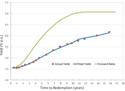
Our ultimate goal is to derive a single discount rate d which we can use to discount future cash flows. The first step is to model a forward rate curve
from which we derive the discount rate curve. To check if our model is
the data best.
To model to forward curve we will use a cubic spline. A cubic spline is a
piece-wise polynomial function. It consist of different segments joined together at
different points or knots. The knots are chosen by the user before modeling.
If there are two knots {k1, k2}, then the piecewise cubic polynomialS(t) has the following form
S(t) = 8 > > > > <
> > > > :
a0 +a1t+a2t2+a3t3 for t≤k1
b0 +b1(t−k1) +b2(t−k1)2+b3(t−k1)3 for t∈[k1, k2]
c0+c1(t−k2) +c2(t−k2)2+c3(t−k2)3 for t≥k2.
(14)
Naturally, the first two equations should be equal at k1 in order to produce a smooth curve. Additionally, at k1, the first and second derivative should be equal as well. This is essential for pricing debt securities and hence one
of the reasons why cubic spline methodology is appropriate to model interest
rates. Similarly the latter two equations should be equal at point k2. We want to find the set of parameters that provide the best fit to the observed
bond prices.
In our list of government bonds the maximum time to maturity is 16 years.
We will run through every possible combination of knots, in increments of 0.5, to find the best fit. To measure the goodness of fit we will define a ”loss”. The
best fit is then a set of parameters {a0, . . . , a3, b0, . . . , b3, c0, . . . , c3} together with two knots {k1, k2} that minimizes the loss.
the forward curve then we define the loss L as L= 18 X i=1 ✓
fi(S(t))−Pi
DM Ti
◆2
, (15)
that is the loss is defined as the squared difference between the market price
and the fitted price weighted by the inverse square of the discounted mean
term (DMT). The discounted mean term is defined as
DM Ti =
P
jtijcijvtij
P
jcijvtij
. (16)
Recall that cij is the the jth cash flow of bondi made at time tij. The last
term vtij is the discount factor. If we have modeled our forward curve by the cubic spline S(t) then the price of bond i according to the spline is
fi(S(t)) =
X
j
cije
Rtij
0 S(t)dt. (17)
As mentioned before we will consider every possible combination of knots in
increments of 0.5 to minimize the loss L. For the two knots {k0
1, k02} with the smallest loss we again run through every possible combination of knots
of increments 0.1 in the intervals (k0
1−0.5, k10+ 0.5) and (k02−0.5, k02+ 0.5) to determine the optimal knots {k1, k2}. The following graph shows the cubic spline representing the forward curve and the corresponding yield curve with
Figure 2: Forward rates, actual and fitted yields.
ft,t+1 for the next 20 years that is for t = 0, . . . ,19. Subsequently we can derive the discount rates:
dt+1 =
t
Y
t0=0
(1 +ft0,t0+1) 1, (18)
for t = 0, . . . ,19. The cash flows for ABC are projected quarterly, hence we want quarterly discount rates. Assuming that payments on average occur at
the midpoint of each quarter, the discount rate for the first quarter d0.25 is approximately (1 +f0,1)
1
8. The discount rates for the following quarters are
then recursively defined as
d0.25(T+1)=d0.25T ×(1 +ft,t+1)
1
for T = 1, . . . ,80 and t = 1, . . . ,19 and where d0.25T is the discount rate for
the quarter ending at time 0.25T. Finally, we want to select a single discount
rate d which we use for discounting future cash flows :
80 X
T=1
CF0.25T
1 +d0.25T
= 80 X
T=1
CF0.25T
1 +d , (20)
where CF0.25T is the cash flow in the quarter ending at time 0.25T. In our
example for ABC the solution of (20) isd = 3.14%, we adopt a discount rate of d= 3.15%.
Note that in this example for ABC we have to make a small adjustment when
calculating the one-year forward rates ft,t+1 and the discount rates dt as the
list of 18 government bonds is from 21 June 2013 and our valuation is due
at 30 June 2013. Time t = 0 corresponds to 21 June 2013, but we actually want t to start 9 days later at 30 June 2013. Since 3659 ≈ 0.025 we could approximate dt+0.025 by
dt+0.025 =dt×(1 +ft,t+1) 0.025, (21)
for t= 0, . . . ,19 and setting d0 = 1. Then
ft+0.025,t+1.025 =
dt+0.025
dt+1.025
From here we can calculate the quarterly discount rates and eventually the
single discount rate d.
Since the future value of a cash flow CF m years from now is
CF
✓ 1 +i
1 +d
◆m
, (23)
we are particularly interested in the difference between the adopted single
interest rate and the adopted single discount rate. The difference in our
example is 3.50%−3.15% = 0.35%. As we had an inflation rate of 3.45% and a discount rate of 2.80% last year the gap decreased by 30 basic point, resulting in a decrease in the outstanding claim provision.
Now, one might wonder why we use a cubic spline and not (segments of) a
second, fourth or higher order spline to model the forward rate curve. This is
because when creating a spline passing trough a number of predefined knots
one wants to minimize the curvature. For a function f(x) on an interval [x0, xn] going through n + 1 points (in our model we have 18 points, so
n = 17) that (approximately) corresponds to minimizing
I[y(x)] = Z b
a
[f00
(x)]2dx. (24)
There exists a general procedure (see L. Elsgolc (1962) for a derivation) to
f(x),f0(x) and its successive derivatives i.e.,
v[y(x)] = Z b
a
G[f(x), f0
(x), . . . , f(n)(x)]dx. (25)
Note that expression (24) is a simple form of (25) whereG(·) = (·)2and where all arguments f(n)(x) are missing except f00(x). Now a general solution for
(25) is given in the form of the Euler-Poisson equation. If y(x) minimizes
v[y(x)], it has to be the solution of the following Euler-Poisson equation:
d dyG−
d2
dxdy0G+ d3
dx2y00G+. . .+ (−1)
n dn+1
dxndy(n)G= 0. (26)
Now in our case only the term y00 = f00(x) exists, so formula (26) simplifies
to
d3
dx2dy00G= 0.
Since G= [f00(x)]2, we have d
dy00G= 2f
00(x). Then
d dx22f
00
(x) = 2f(4)(x) = 0. (27)
So f(4)(x) = 0. Integrating this term 4 times we obtain f(x) = a
0 +a1x+
3.3
Superimposed Inflation
Benefits for personal injury tend to increase faster than the normal inflation
rate. This additional increase is called superimposed inflation. Superimposed
inflation can have various causes, for example; a legal decision increases the
average benefit for a certain injury or allows a larger group of claimants access
to a particular head of damage. Or a claimant can get access to a particular
head of damage due to better preparation by their lawyers. Another cause
can be the change in the treatment for a particular injury, which can imply
an increase or decrease in costs. To detect superimposed inflation from the
data one can examine whether the average claim payments in current values
show a trend. If the average claim payments tend to increase over time one
might introduce superimposed inflation. In the analysis for ABC we do not
adopt any superimposed inflation rate.
3.4
Expense Rate
When calculating the outstanding claims liability we allow for claims
hand-ling expenses. This expense rate is often provided by the client.
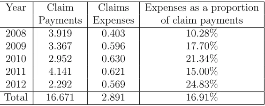
Unfortu-nately, ABC does not provide us with an estimate of the claims handling
expense, but instead provides us with the following table containing the
to-tal expenses over the last five years.
To decide what proportion relates to the claims handling we look at results
Year Claim Claims Expenses as a proportion Payments Expenses of claim payments
2008 3.919 0.403 10.28%
2009 3.367 0.596 17.70%
2010 2.952 0.630 21.34%
2011 4.141 0.621 15.00%
2012 2.292 0.569 24.83%
Total 16.671 2.891 16.91%
Table 3: Total expenses for ABC in millions
that the total expenses paid were $548.904 million. That is about 35% of the $1,562.396 million claim payments. The total allowance for claims
handling expenses reported is 11.8%, which represents about one third of
the total expenses. An obvious approach to calculate the claims handling
expenses from the above table would be to use a similar proportion, that
would result in a claim handling expense rate somewhere between 3.4% and 8.3%. We adopt a conservative claim handling expense rate of 8%. This is considering the possibility that the proportion of the claim handling expense
rate for self-insurers is higher than the considered similar self-insurer.
4
Grossing up the Data
The review of the outstanding Victorian workers’ compensation liabilities of
ABC as at 30 June 2013 has been prepared based on transaction data to 30
need to gross up the number of claims reported, the gross claim payments
and the gross case estimates. For this we use the the chain ladder factor
and incurred cost development factor which we discuss more extensively in
section 6.1 and 6.4.
To approximate the grossed-up payments for each accident quarter we can
multiply the projections from last year’s valuation by 2/3 and add them to
the payments made in April 2013.
In order to determine the grossed up case estimates we first estimate the
grossed up incurred costs. The incurred costs are the sum of the gross claim
payments and the case estimates. Let Wid denote the incurred cost for
ac-cident quarter i and development quarter d and let ςj be the corresponding
incurred cost development factor (see section 6.4 and (42) how to select ςj).
The grossed up incurred cost is simply Wid×ςd. Subsequently the grossed
up case estimate is equal to the grossed up incurred cost minus the grossed
up claim payments.
If the ultimate number of claims expected from last times valuation for the
second quarter of 2013 was N, then the number of expected claims reported in this quarter is the result of
N
Q
d 2δd
, (28)
where δd is the chain ladder factor for the projected number of claims (see
claims reported in the second quarter of 2013 from the first quarter of 2013
is N ×(δ2 −1). For earlier accident quarters we have a table with adopted future number of claims in our previous valuation. Now that we have all
expected numbers for the second quarter of 2013 and every accident quarter
we can calculate the grossed up number of claims reported by adding 2/3 of the expected number of claims reported to the actual number of claims
reported in the month April.
5
Projected Number of claims
In the first part we outputted a triangle containing the number of claims
reported for each accident and development period. In our example the
period is a quarter. Let I be the current accident quarter and Nid is the
number of claims reported in accident quarter i, for i = 1, . . . , I with delay
d, whered= 0, . . . I−i. This will give us an upper triangle with observations
{Nid :i+d ≤I}. Our goal is to predict the number of claims reported Nid
where i+d > I. In order to do so we first calculate the ratios between the number of claims reported in successive development quarters;
ρid=
Pd
j=0Nij
Pd 1
j=0Nij
(29)
quarter d this expression simplifies to
ρid=
Ni,d
Ni,d 1
. (30)
This will produce an upper triangle that provides us an overview containing
all ratios between the number of claims reported in successive development
quarters from the past. To project the number of claims reported into the
future we determine one factor for each development quarter. In our example
for ABC we calculate these factors with respect to the last 4, the last 8, the
last 12 and all accident quarters. For all accident quarters this is defined as
δdALL=
PI d
i=1 Ni,d
PI d
i=1 Ni,d 1
. (31)
That is, the chain ladder factor δALL
d represents the average relative increase
in the reported proportion from development period d−1 to development period d. Based on these chain ladder factors calculated with respect to different time periods (last 4, 8 and 12 quarters) the appointed actuary will
choose the factors δd he thinks predicts the data best. Subsequently we
can project the number of claims reported Nid for accident quarter i and
development quarterd, wherei+d > I, with the following recursive formula:
Nid=
8 > <
> :
Ni,d 1×(δd−1) if i+d=I+ 1
Ni,d 1×(δd−1) if i+d > I + 1.
6
Valuation Methods
In order to predict the future cash flows and liabilities we use several valuation
methods. Here follows a discussion of the different methods used:
6.1
Chain Ladder Method
In the same way as we projected the number of claims reported we can
project the gross claim payments. We use formula (30), where we replace
the number of claims reported Nid in accident quarter i and development
quarter d by the gross claim payments Yid to create an upper triangle
con-taining all ratios between gross claim payments in consecutive development
quarters. Subsequently we calculate the chain ladder factors using formula
(31), replacing the number of claims reported Ni,dand Ni,d 1 byYi,d and
Yi,d 1 respectively. Again, based on his experience, the appointed actuary will select a chain ladder factor he believes reflect the data best. With the
selected chain ladder factors we predict the inflated future claim payments
Yid, for i+d > I, as we did with the numbers of claims reported:
Yid=
8 > <
> :
Yi,d 1 ×(δd−1) if i+d=I+ 1
Yi,d 1×(δd−1) if i+d > I + 1.
(33)
Subsequently we inflate and discount the projected claim payments to, in this
6.2
PPCI Method
In the payment per claim incurred (PPCI) method we look at the
devel-opment of the payment per claim Yid(k) instead of the total claim payments
Yid as we did in the previous method. From the gross claim payments we
first calculate the average gross payments per claim incurred ˆYid by simply
dividing the gross claim paymentsYidfor accident quarteriand development
quarter d by the estimated ultimate number of claims reported in accident year i i.e.,
ˆ
Yid =
Yid
Ni,I 1
, (34)
where i+d ≤ I. This will produce an upper triangle with gross payments per claim incurred for each accident and development quarter. We would
like to select one value for each development quarter that we use to project
the PPCIs into the future. Therefor we calculate the average gross payment
per claim incurred over all accident quarters:
ˆ
Yd ALL
=
PI d
i=1 Yˆid
PI d
i=1 Ni,I 1
(35)
for each development quarter d ≥ 1. In our case of the valuation of ABC we also calculate an average for the last 4, 8 and 12 accident years. The
appointed actuary will then select one ˆYd for each development quarter d
project the inflated gross claim payments into the future we use the projected
number of claims from part 5:
Yid = ˆYd×Ni,I 1, (36)
for i +d > I. Finally we inflate and discount the projected gross claim payments to June 2013 values.
6.3
PPCF method
In the PPCI method we projected the claim payments per claim incurred, in
the PPCF method we project the claim payments per claim finalized. From
the data received by our client we can extract the number of open claimsOid
and finalized claimsFidfor every accident quarteriand development quarter
d, wherei+d≤I. The first step is to estimate the probabilityωdthat a claim
is finalized with delay d. Therefor we produce a triangle containing ratios
ωij of finalized claims to the total number of claims reported for i+d ≤I,
ωid=
8 > > > > <
> > > > :
Fid
Nid if d= 0
Fid
Nid+Oi(d 1) if d ≥1,
(37)
will select a ωd for every development quarter d, that is the probability of
a claim being finalized in development quarter d. Using this probability we can estimate the number of finalized claims Fid for i+d > I:
Fid =ωd×Nid×P[claim finalized]. (38)
In our example the probability that a claim is finalized is set at 100%. We can
then calculate the average gross payment per claim finalized ˆYidf by dividing the gross claim payments Yid by the ultimate number of claims finalized in
the corresponding accident and development quarter:
ˆ
Yidf = Yid
Fid
. (39)
Based on this triangle we select one payment per claim finalized ˆYdf for every development quarter d that we use to project the future cash flows Yid:
Yid = ˆY f
d ×Fid, (40)
for every i+d > I.
6.4
ICD method
In the incurred cost development (ICD) method we look at the incurred
costs instead of just the gross claim payments. The total incurred costs Wid
Wid =Yi,d+Vid, where Vid is the case estimate andYi,d is the cumulative
payment for accident year i up to development quarter d. As for the chain ladder method we want to select a development factor which in this case
we use to project the future incurred costs. To do so, we first create a
corresponding triangle to the triangle of inflated incurred costs containing
all ratios between consecutive development quarters:
ςid=
Wid
Wi(d 1)
, (41)
where i+d ≤ I. To select one development factor for each development quarter we calculate an average incurred cost development factor over all
accident years:
ςdALL=
PI d
i=1 Wid
PI d
i=1 Wi(d 1)
, (42)
for every 1≤d < I. For ABC we calculate a similar average over the last 4, 8 and 12 years and the actuary will select an incurred development factorςd
for each development period based on his experience. The projected incurred
costs Wid for i+d > I are calculated as follows:
Wid =
8 > <
> :
Wi(d 1)×ςd if i+d =I+ 1
Wi(d 1)×ςd if i+d > I + 1
Subsequently we produce the tables containing the inflated and discounted
to June 2013 incurred costs.
6.5
PCE method
In the projected case estimate (PCE) method we first project the case
esti-mates into the future and use these to project the gross claim payments.
The first step in the PCE method is to compute the payment to outstanding
factors νid, for i+d ≤I. The payment to outstanding factor is the ratio of
inflated gross payment of this quarter to the inflated gross case estimates of
last quarter i.e.,
νid =
Yid
Vi(d 1)
. (44)
We want to select one payment to outstanding factorνdfor each development
period d. To give us an indication of what value to select we calculate the average payment to outstanding factors over the last 4, 8, 12 and all accident
quarters. The average over all accident quarters is calculated as follows:
νdALL =
PI d
i=1 Yid
PI d
i=1 Vi(d 1)
, (45)
follows
ξid =
Yid+Vid
Vi(d 1)
. (46)
That is, the case estimate development factor measures how the previous
case estimate has progressed since last quarter. Some part of last years case
estimate will have been actualized into payments. If case estimates were
constant over time then Vid =Vi(d 1)−Yid, however, in reality case estimates
tend to vary over time due to new available information. That is why we
calculated the payment to outstanding factors; these factors will help us
identify what part of the change in case estimates comes from payments made
and what change comes from revision of the case estimate and\or new claims. To help us select an appropriate case estimate development factorξdfor every
development quarter d we again calculate four averages over different time periods. The average over all accident quarters for development quarter d is the result of
ξdALL = PI d
i=1 Yid+
PI d
i=1 Vid
PI d
i=1 Vi(d 1)
, (47)
for 1≤d < I. The appointed actuary will then select a payment to outstand-ing factorνdand a case estimate development factorξdfor each development
after which the factors νd will approach 1 or equal 1. Now, the difference
between the case estimate development factor and the payment to
outstand-ing factor i.e., ξd−νd, will reflect the change in case estimate due to new
available information and/or new claims. So to project our case estimates in the future, that is calculating Vid for all i+d > I we use the recursively
defined formula
Vid=
8 > <
> :
Vi(d 1)×(ξd−νd) if i+d=I + 1
Vi(d 1)×(ξd−νd) if i+d > I + 1.
(48)
To project the inflated gross claim payments into the future we use the
(projected) case estimates and the payment to outstanding factors:
Yid =
8 > <
> :
Vi(d 1)×νd if i+d =I+ 1
Vi(d 1)×νd if i+d > I + 1.
(49)
6.6
BF method
One significant difference in the Bornhuetter-Ferguson (BF) spread-sheet
model used in our valuation from the models previous discussed is that we
include the exposure in the analysis. The exposure in this case is defined as
the earned premium. In this method we will calculate the total amount of
outstanding claims for each accident quarteri. Subsequently we will identify a payment pattern using delay probabilities which we will use to project to
Our first step is to calculate the ultimate incurred costs for each accident
quarter i. To do so we first compute the cumulative incurred cost develop-ment factors γi from the incremental incurred development factors ςd
calcu-lated in section 6.4;
γi = I 1 Y
d=I i
ςd, (50)
for every accident quarter i ≥ 1. From (43) we can calculate the IBNR factors IBN Ri :
IBN Ri =
1 1−γi
. (51)
Now, let pi be the earned premium in accident quarter i. The ultimate
incurred costs µi for accident quarter i can be calculated with the following
formula:
µi = I i
X
d=1
Wid+ρi×γi×LRi, (52)
where LRi is the selected loss ratio for accident quarter i. The appointed
actuary will then select a loss ratio based on prior experience. To assist in the
loss ratios
LRid =
Wid
pi
, (53)
for i+d ≤ I, that is for accident quarter i and development quarter d the loss ratio is defined as the incurred costs divided by the premium earned in
accident year i.
With the ultimate incurred costs, we can calculate the outstanding claims
OSCi for each accident quarter i by simply subtracting the gross claim
pay-ments:
OSCi =µi− I i
X
d=1
Yid. (54)
The next step is to identify a payment pattern. One of the possibilities is to
calculate the incremental delay probabilities from the chain ladder
develop-ment factors calculated in section 6.1.
We first calculate the cumulative development factors
∆d =
d
Y
j=1
δj (55)
for 1 ≤ d < I. The second step is to calculate the cumulative delay proba-bilities
Λd= ∆
d
∆I
The incremental delay probabilityλd=Λd−Λd 1. All delay probabilities λd,
with P
dλd = 1, form a payment pattern. Instead of using the chain ladder
development factors, we could also use the selected PPCIs ˆYd from section
6.2 to calculate the delay probabilities:
λd=
ˆ
Yd
PK
d=1Yˆd
. (57)
Then the projected number of claims can be calculated as follows
Yid =λd×OSCi, (58)
for i+d > I.
Having calculated the future cash flows and liabilities according to the several
methods we have to choose which method, or combination of methods, we
use in our report to the client. We do this by allocating weights wik to each
accident quarter i and every method k. In general we give more weight to methods based on case estimates in early years, like the ICD method and
more weight to a method based on averages in more recent years, like the
PPCI method. Case estimates tend to be more accurate in earlier years as
future claims reports are not anticipated whereas in more recent years there
6.7
Results
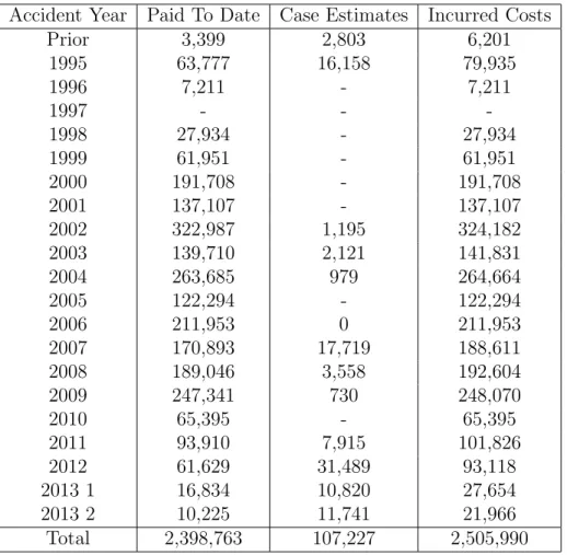
For ABC we used the Chain Ladder, PPCI and the ICD method to value
out-standing claims. Table 4 shows the actuarial statistics with the amounts paid
to date, case estimates and the incurred costs. Table 5 shows the ultimate
claim payments according to the different methods.
Accident Year Paid To Date Case Estimates Incurred Costs
Prior 3,399 2,803 6,201
1995 63,777 16,158 79,935
1996 7,211 - 7,211
1997 - -
-1998 27,934 - 27,934
1999 61,951 - 61,951
2000 191,708 - 191,708
2001 137,107 - 137,107
2002 322,987 1,195 324,182
2003 139,710 2,121 141,831
2004 263,685 979 264,664
2005 122,294 - 122,294
2006 211,953 0 211,953
2007 170,893 17,719 188,611
2008 189,046 3,558 192,604
2009 247,341 730 248,070
2010 65,395 - 65,395
2011 93,910 7,915 101,826
2012 61,629 31,489 93,118
2013 1 16,834 10,820 27,654
2013 2 10,225 11,741 21,966
Total 2,398,763 107,227 2,505,990
Table 4: Actuarial Statistics.
sev-Accident Year Chain Ladder PPCI ICD Selected
Prior 3,416 3,411 6,201 6,201
1995 64,298 63,805 79,935 79,935
1996 7,293 7,279 7,211 7,211
1997 - 124 -
-1998 28,411 28,113 27,934 27,934
1999 63,087 62,186 61,951 61,951
2000 195,678 192,036 191,708 191,708 2001 140,551 137,411 137,107 137,107 2002 332,334 323,407 324,182 324,182 2003 144,292 140,355 141,831 141,831 2004 273,421 265,724 264,664 264,664 2005 127,318 124,163 122,294 122,294 2006 221,566 215,041 211,953 211,953 2007 180,291 174,285 188,611 188,611 2008 202,746 196,466 192,604 192,604 2009 270,690 257,145 248,070 248,070
2010 73,017 72,728 65,395 65,395
2011 108,138 104,714 101,826 101,826
2012 90,172 72,434 93,118 93,118
2013 1 23,089 14,132 21,045 21,045
2013 2 49,246 28,617 24,773 28,617
Total 2,599,054 2,483,577 2,512,412 2,516,256
Table 5: Ultimate claim payments according to the three different methods.
eral methods we have to choose which method, or combination of methods,
we use in our final valuation. We do this by allocating weights wik to each
accident quarter i and every method k. In general we give more weight to methods based on case estimates in early years, like the ICD method and
may be a significant number of IBNR claims.
ABC still has open claims from accident quarters before 1995 1 (grouped as
”prior”) and 1995 3. The ICD method, based on case estimates, projects
sig-nificant payments relating to these accident quarters, whereas the payments
according to the CL and PPCI methods are negligible. These methods ignore
the number of open claims and their case estimates. Hence we allocate 0%
to the CL and PPCI method to early accident quarters, in fact, for ABC
we allocate 0% to all quarters except for the last quarter 2013 2. For the
last quarter we allocate 100% to the PPCI method. The projected claim
payments in the last quarter according to the PPCI method are higher then
projected by the ICD method. The amount in the last quarter according to
the ICD method may not be sufficient as a number of claims are incurred,
but not yet reported, and hence they are not included in the case estimates.
The high amount predicted by the CL method seems unreasonably high when
comparing to previous results. The ultimate claim payments projected by
the chain ladder method (2,599,054) are much higher than projected by the
PPCI method (2,483,577) and the ICD method (2,512,412). The chain
lad-der method, only depending on amounts to date, gives volatile forecasts,
7
Risk Margin
The risk margin according to APRA should give 75% adequacy. To calculate
the risk margin for ABC we use a Bayesian model for the PPCI method.
In Bayesian statistics the selected PPCIs ˆYd for each development quarter d
from section 6.2 become distributions themselves, making allowance for the
volatility in the data. Each column of PPCIs becomes the data points for
the distribution for the selected PPCIs. So for development quarter d the data points (from (34)) are ˆY1d, . . . ,Yˆ(I d)d. We use an uninformative prior,
i.e. the prior information does not influence the result of the model. So the
model is completely driven by the observed experience ˆYid, wherei+d≤I.
(This in contrast to an informative prior which could be something like ”The
average PPCI for the first development quarter is about $5,000”.)
For every development quarter d we have to fit a distribution to the data points. In case of ABC the best fit is a normal distribution. The optimal
parameters can be found by minimizing the log-likelihood function. In case of
the normal distribution the optimal parameter for the mean for development
quarter d is the simple average of the PPCIs with delay d. Using the simple average and the standard deviation we simulate the outstanding claims 1000
times. This Bayesian model gives us the full distribution of the outstanding
8
Reinsurance
In case of ABC the entire portfolio of business is reinsured on an excess of loss
basis. ABC may recover losses on an individual risk in excess of $750.000. ABC estimated recoveries in respect to two large claims. As the number
of large claims reported are very small and the average payments per large
claim incurred is about $280.000, no further allowance is made. If recoveries are more frequent, a valuation method such as the PPCI could be used to
References
Bolder, D Gubsa, S (2002): ”Exponentials, Polynomials and Fourier Series:
More Yield Curve Modelling at the Bank of Canada.” Working Paper of the
Bank of Canada.
Cutter, K (2009, November): ”Measuring and Understanding Superimposed
Inflation in CTP Schemes.” Paper presented at the 12th Accident
Compen-sation Seminar of the Institute of Actuaries (Australia), Melbourne, Victoria.
De la Grandville (2001): ”Title of work: Bond pricing and portfolio
anal-ysis.” Place of publication: The MIT Press.
L. Elsgolc (1962): ”Title of work: Calculus of Variations.” Place of
publica-tion: Dover Publications.
Miller, H (2010): ”Towards a better inflation forecast.” Paper presented at
the 17th General Insurance Seminar of the Institute of Actuaries (Australia),
Gold Coast, Queensland.
Neuhaus, W. (2013): ”Outstanding Claims in General Insurance.”
Pienaar, R Choudry, M : ”Fitting the term structure of interest rates: the
practical implementation of cubic spline methodology.” Paper of the Deutsche