Electronic Appendix (Introduction to R)
Ken Aho
Foundational and Applied Statistics for Biologists Using R (electronic appendix)
INTRODUCTION TO R
Ken Aho
CRC Press
Taylor & Francis Group
6000 Broken Sound Parkway NW, Suite 300 Boca Raton, FL 33487-2742
© 2014 Taylor & Francis Group, LLC
Contents
1 Introduction to R ������������������������������������������������������������������������������������������������������������������ 1
1.1 A very brief history ...1
1.2 The
R
language ...2
1.3
R
copyrights and licenses ...2
1.4
R
and reliability ...2
1.5 Installation ...3
2 Basics ��������������������������������������������������������������������������������������������������������������������������������������� 4
2.1 First operations ...4
2.2 Use your scroll keys ...5
2.3 Note to self:
#
...5
2.4 Unfinished commands ...6
2.5 Basic options ...6
2.6 Saving and loading your work ...7
3
Geting help in R
����������������������������������������������������������������������������������������������������������������� 10
3.1
help
...10
3.2 Manuals and additional information ...11
4
Expressions and assignments
������������������������������������������������������������������������������������������� 13
4.1 Naming objects ...13
4.2 Combining objects with
c
...14
5
R objects and R classes
������������������������������������������������������������������������������������������������������� 15
5.1 Listing objects ...16
6
Mathematical operations
��������������������������������������������������������������������������������������������������� 17
6.1 Mathematical operators and functions ...17
6.2 Statistical operators ...21
7
R packages
��������������������������������������������������������������������������������������������������������������������������� 23
7.1 Datasets in packages ...25
8
R and spreadsheets
������������������������������������������������������������������������������������������������������������� 28
8.1
attach
and
detach
...28
8.2
with
...29
8.3
remove
and
rm
...29
8.4 Cleaning up ...29
9
R graphics
����������������������������������������������������������������������������������������������������������������������������� 30
9.1
plot
...30
9.2 Scatterplots ...35
9.3 Graphical devices ...36
9.5 Exporting graphics ...38
9.6 Typeface families ...39
9.7
text, lines, points, paste
...41
9.8
plotmath
...42
9.9
axis
...42
9.10
mtext
...43
9.11 Histograms ...46
9.12 Subsetting scatterplot arguments using a categorical variable ...48
9.13 Plotting variables using additional axes ...50
9.14 Barplots ...51
9.15 Multivariate line and scatterplots ...55
9.16 Boxplots ...57
9.17 Interval plots ...58
9.18 Three dimensional plots ...59
9.19 Auxiliary graphics packages ...62
10 Data structures ��������������������������������������������������������������������������������������������������������������������68
10.1 Vectors ...68
10.2 Matrices ...69
10.3 Arrays ...69
10.4 Dataframes ...70
10.5 Lists ...71
11
Data entry at the command line
�������������������������������������������������������������������������������������74
11.1
scan
,
cbind
,
rbind
...74
11.2 Facilitating command line entry:
seq
and
rep
...75
12
Importing data into R
��������������������������������������������������������������������������������������������������������76
12.1
read.table
...76
12.2
read.csv
...77
12.3
scan
...77
12.4 Easy imports: use of
file.choose()
...77
12.5 Additional comments ...77
13
Exporting data from R
�������������������������������������������������������������������������������������������������������79
14
Subseting matrix, dataframe and array components
�������������������������������������������������80
15
Operations on matrices and dataframes
����������������������������������������������������������������������82
15.1
apply
...83
15.2
tapply
...84
15.3
outer
...84
15.4
lower.tri
,
upper.tri
and
diag
...85
16
Logical commands
�������������������������������������������������������������������������������������������������������������87
16.1
ifelse
...88
16.2
if
,
else
,
any
, and
all
...88
17
Simple functions for data management
�����������������������������������������������������������������������89
17.1
replace
...89
17.2
which
...89
17.3
sort
...90
17.4
rank
...90
17.5
order
...90
17.6
unique
...91
17.7 match
...92
17.8
which
and
%in%
...93
17.9
strsplit
and
strtrim
...93
17.10 Complex pattern matching:
gsub
,
grep,
and metacharacters ...94
18
Testing and coercing
����������������������������������������������������������������������������������������������������������96
19
NA
,
NaN
, and
NULL
��������������������������������������������������������������������������������������������������������98
20
Binary numbers, bits and bytes
�������������������������������������������������������������������������������������101
20.1 Floating point arithmetic ...102
20.2 Binary characters ...104
21
Writing functions
�������������������������������������������������������������������������������������������������������������105
21.1 An introductory example ...106
21.2 Global variables versus local variables ...107
21.3
uniroot
...110
21.4
switch
...110
21.5 Triple dot
...
argument ...111
21.6 Looping ...117
21.7 Looping without
for
...121
21.8 Calling and receiving code from other languages ...121
21.9 Functions with animation ...124
21.10 Building GUIs ...128
21.11 Functions with
class
and
method
...131
21.12 Documenting functions and workflow ...132
22 Exercises �����������������������������������������������������������������������������������������������������������������������������137
I believe that R currently represents the best medium for quality software in support of data analysis.
John Chambers, a developer of S
R is a real demonstration of the power of collaboration, and I don’t think you could construct something like this any other way.
Ross Ihaka, original co-developer of R
1 Introduction to R
R is a computer language and an open source seting for statistics, data management, computation, and graph -ics. The outward mien of the R-environment is minimalistic, with only low-level interactive facilities. This is in contrast to conventional statistical software consisting of extensive, high-level, often inlexible tools. The simplicity of R allows one to easily evaluate, edit, and build procedures for data analysis.
R is useful to biologists for two major reasons. First, it provides access to a large number of existing statisti-cal, graphistatisti-cal, and organizational procedures, many of which have been designed speciically for biological research. Second, it allows one to “get under the hood”, look at the code, and check to see what algorithms are doing. If, after examining an R-algorithm we are unsatisied, we can generally modify its code or create new
code to meet our speciic needs.
1�1
A very brief history
R was created in the early 1990s by Australian computational statisticians Ross Ihaka and Robert Gentleman to address scoping and memory use deiciencies in the language S (Ihaka and Gentleman 1996). At the insistence of Swiss statistician Martin Maechler, Ihaka and Gentleman made the R source code available via the internet in 1995. Because of its relatively easy-to-learn language, R was quickly extended with code and packages devel-oped by its users (§ 7). The rapid growth of R gave rise to the need for a group to guide its progress. This led, in 1997, to the establishment of the R-development core team, an international panel that modiies, troubleshoots,
and manages source code.
Because of its freeware status, the overall number of R-users is diicult to determine. Nonetheless, experts in
the computer industry estimated that between 1 and 2 million individuals were actively using R in 20091. This number has undoubtedly increased as the number of R-packages has continued to increase exponentially (Fox 2009). Other reports indicate that the internet traic for R topics exceeds discussions for all other types of sta-tistical software2. In addition, recent searches using Google scholar® (htp://scholar.google.com/) show that the number of citations of R and its packages in scientiic articles has increased dramatically since 2005 while
citations for software giants SAS® and SPPS® have declined3,4. R is currently the most popular programming language in the world among data scientists5, and is ranked 6th in world by the Institute of Electrical and
Elec-1htp://bits.blogs.nytimes.com/2009/01/08/r-you-ready-for-r/ accessed 9/1/2017 2htp://r4stats.com/articles/popularity/ accessed 9/1/2017.
3htp://www.r-bloggers.com/rs-continued-growth-in-academia/ accessed 9/1/2017
4For additional information on the historical and technical development of R see Hornick (2009) and Venebles et al.
(2008).
tronics Engineers (IEEE) for general programming use6.
1�2
The R language
The R language is based on the older languages S, developed at Bell Laboratories (Becker and Chambers 1978, Becker and Chambers 1981, Becker et al. 1988), Scheme, developed initially at MIT (Sussman and Steele 1975, Steele 1978), and Lisp, also developed at MIT (McCarthy et al. 1960). Ihaka and Gentleman (1996) used the name
R both to acknowledge the inluence of S (because R and S are juxtaposed in the alphabet), and to celebrate their
personal eforts (because R was the irst leter of their irst names). S has since been adapted to run the commer -cial software S-Plus®. The R and S languages remain very similar, and code writen for S can generally be run
unaltered in R. The method of function implementation in R, however, remains more similar to Scheme.
R difers from S in two important ways (Ihaka and Gentelmen 1996). First, the R-environment is given a ixed
amount of memory at startup. This is in contrast to S-engines which adjust available memory to session needs. Among other things, this diference means more available pre-reserved computer memory, and fewer virtual pagination7 problems in R (Ihaka and Gentelmen 1996). It also makes R faster than S-Plus for many applications (Hornik 2009). Second, R variable locations are lexically scoped. In computer science, variables are storage
areas with identiiers, and scope deines the context in which a variable name is recognized. So-called global variables are accessible in every scope (for instance, both inside and outside functions). In contrast, local vari
-ables exist only within the scope of a function. Formal parameters deined in R functions, including arguments, are (generally) local variables, whereas variables created outside of functions are global variables. Lexical scop-ing allows functions in R access to variables that were in efect when the function was deined in a session. S,
however, does not allow such free variables. The characteristics of R functions and details concerning lexical scoping are further addressed in § 21.
1�3 R
copyrights and licenses
R is free, and as a result there are no warranties on its environment or packages. As its copyright framework R
uses the GNU (a recursive acronym for GNU is not Unix) General Public License (GPL). This allows users to share and change R and its functions. The associated legalese can read by typing RShowDoc("COPYING")in the R-console. Because its functions can be legally (and easily) recycled and altered we should always give credit to developers, package maintainers, or whoever wrote the R functions we are using.
1�4 R and
reliability
The lack of an R warranty has frightened away some scientists. But be assured, with few exceptions R works as well or beter than “top of the line” analytical commercial software. Indeed, SAS® and SPSS® have recently made R applicationsaccessible from within their products (Fox 2009). For specialized or advanced statistical techniques R often outperforms other alternatives because of its diverse array of continually updated applica-tions.
The computing engine and packages that come with a conventional R download (see § 1.5) meet or exceed U.S.
6htp://spectrum.ieee.org/computing/software/the-2017-top-ten-programming-languages accessed 9/1/2017 (currently, the big ive are, from irst to last, Python, C, Java, C++, and C#)
7 Virtual pagination is a memory management scheme that allows a computer to store and retrieve data from secondary
federal analytical standards for clinical trial research (R Foundation for Statistical Computing 2008). In addition, core algorithms used in R are based on seminal and trusted functions. For instance, R random number genera-tors include some of the most venerated and thoroughly tested functions in computer history (Chambers 2008). Similarly, the LAPACK algorithms (Anderson et al. 1999), used by R for linear algebra, are among the world’s most stable and best-tested software (Chambers 2008).
1�5
Installation
To install R, irst go to the website htp://www.r-project.org/. On this page specify which platform you are using (Figure 1, step 1). R can currently be used on Unix-like, Windows and Mac operating systems. This appendix has been created speciically for Windows users of R. In almost every case, however, it will also be applicable to other platforms. Once an operating system has been selected one can click on the “base” link to download the precompiled base binaries if R currently exists on your computer. If R has not been previously installed on your computer click on "Install R for the irst time" (Figure 1, step 2). You will delivered to a window containing a link to download the most recent version of R. Click on the "Download" link (Figure 1, step 3).
Figure 1Method for installing R for the 1st time.
2 Basics
Upon opening R two things that will appear in the console of the Graphical User Interface (R-GUI). These are the license disclaimer and the command line prompt, i.e., > (Figure 2). The prompt indicates that R is ready for a command. All commands must begin at >. R user commands are colored red, and output, including errors and warnings are colored blue.
We can exit R at any time by typing q() in the console, closing the GUI window (non-Unix only), or by select-ing “exit” from the pulldown File menu (non-Unix only).
Figure 2 The R console. R version 2.15.1, "Roasted Marshmallows"
2�1
First operations
As an introduction we can use R as a calculator. Type 2 + 2 and press Enter.
2 + 2 [1] 4 >
The [1] means, “this is the irst requested element”. In this case there is just one requested element, 4, the solu -tion to 2 + 2. If the output elements cannot be held on a single console line, then R would begin the second line of output with the element number comprising the irst element of the new line. For instance, the command rnorm(20) will take 20 random samples from a standard normal distribution (see Ch. 3 in the Foundational and Applied Statistics text). We have:
rnorm(20)
[1] 0.73704627 0.06572694 -0.19401659 1.55767302 -0.66656940 -0.63375586 [7] -0.38926816 0.46596203 -0.35382023 0.72729659 0.42944759 -0.50559415 [13] 0.95743654 0.49844963 0.01833043 -0.29257820 -0.56753070 0.25374833 [19] -0.27808670 -0.83199069
>
Multiple commands can be entered on a single line, separated by semicolons. Note, however, that this is consid-ered poor programming style, as it may make your code more diicult to understand by a third party.
A new command can be entered at the prompt or by separating commands with a semicolon. 2 + 2; 3 + 2
[1] 4 [1] 5 >
R commands are generally insensitive to spaces. This allows the use of spaces to make code more legible. The command 2 + 2 is simply easier to read and debug than 2+2.
2�2
Use your scroll keys
As with many other command line environments, the scroll keys (Figure 3) provide an important shortcut in R. Instead of editing a line of code by tediously mouse-searching for an earlier command to copy, paste and then modify it, you can simply scroll back through your earlier work using the upper scroll key, i.e.,
↑.
Accordingly, scrolling down using↓
will allow you to move forward through earlier commands.Figure 3 Direction keys on a keyboard.
2�3
Note to self:
#
R will not recognize commands preceded by #. As a result this is a good way for us to leave messages to our-selves.
# Note at beginning of line 2 + 2
[1] 4
2 + # Note in middle of line + 2
[1] 4
above.
2�4
Unfinished commands
R will be unable to move on to a new task when a command line is uninished. For example, type
2 +
and press Enter. We note that a continuation prompt, by default + , is now in the place the command prompt should be. R is telling us the command is uninished. We can get back to the command prompt by inishing
the function, clicking Misc>Stop current computation or Misc>Stop all computations (non-Unix only), typing
Ctrl-C (Unix only), or by hiting the Esc key (Windows only).
2�5
Basic options
To enhance our experience, we can adjust the appearance of the R-console and customize options that afect
function output. These include the characteristics of the graphics devices, the width of print output in the
R-console, and the number of print lines and print digits. Changes to some of these parameters can be made by going to Edit>GUI Preferences in the R toolbar. Many other parameters can be changed using the options function. To see all alterable options one can type:
options()
To change default options one would simply deine the desired change within parenthesis following the
op-tions function name. For instance, to see the default number of digits in R output I would type:
options("digits") $digits
[1] 7
To change the default number of digits in output from 7 to 5, in the current session I would type:
options(digits = 5)
To establish user defaults for all future sessions one will need to change the R-console ile located (currently)
in the etc directory of the version of R you are using. This can either be done manually, or by using Edit>GUI
Preferences>Save in the R toolbar
By default the R working directory is set to be the home directory of the workstation. The command getwd()
shows the current ile path for the working directory.
getwd()
[1] "C:/Users/User/Documents"
of the directory, or by using pulldown menus, i.e., File>Change dir (non-Unix only).
An .Rproile ile exists in your Windows R/R-version/etc directory. R will silently run commands in the ile
upon opening. By customizing the .Rproile ile one can set options, install frequently loaded non-default packages (§ 7), deine your favorite package repository, and create aliases and defaults for frequently used func -tions.
Here is the content of my current .Rproile ile.
options(repos = structure(c("http://ftp.osuosl.org/pub/cran/")))
.First <- function(){ library(asbio)
cat("\nWelcome to R Ken! ", date(), "\n") }
.Last <- function(){
cat("\nGoodbye Ken", date(), "\n") }
The options(repos = structure(c("http://ftp.osuosl.org/pub/cran/"))) command deines my favorite R-repository. The function .First( ) will be run at the start of the R session and .Last( ) will be run at the end of the session. As we go through this primer it will become clear that these functions force R to say hello and to load my package asbio when it opens, and to say goodbye when it closes (although the farewell will only be seen when running R from a command line interface).
The .Rproile ile in the /etc directory is the so-called .Rproile.site ile. Additional .Rproile iles can be
placed in the working and user directories. R will check for these and run them after running the .Rproile. site ile.
One can create .Rproile iles, or any type of R extension ile using the function ile.create. For instance, the code:
ile.create("defaults.Rproile")
places an empty, editable, .Rproile ile called defaults in the working directory.
2�6
Saving and loading your work
As noted earlier, an R session is allocated with a ixed amount of memory that is managed in an on-the-ly man -ner. An unfortunate consequence of this is that if R crashes all unsaved information from the work session will be lost. Thus, session work should be saved often. Note that R will not give a warning if you are writing over another ile from the R console with the same name! The old ile will simply be replaced.
Saving the R History
editable) history window, one would type: history(3)
To save the session history in Windows one can use File>Save History (non-Unix only) or the function savehistory. For instance, to save the session history to the working directory under the name history1 I could type:
savehistory(ile = "history1.Rhistroy")
We can view the code in this ile from any text editor8.
To load the history from a previous session one can use File>Load History (non-Unix only) or the function loadhistroy. For instance, to load history1 I would type:
loadhistory(ile = "history1.Rhistroy")
To save the history at the end of (almost) every interactive Windows or Unix-alke R session, one can alter the
.Rproile ile .Last function to include:
.Last <- function() if(interactive()) try(savehistory("~/.Rhistory"))
Saving R Objects
To save all of the objects (see § 4) available in the current R-session one can use File>Save Workspace (non-Unix
only), or simply type:
save.image()
This procedure saves session objects (see § 4) to the working directory as a nameless ile with an
.
RData extension. The ile will be opened, silently, with the inception of the next R-session, and cause objects used or created in the previous session to be available. Indeed, R will automatically execute all .RDatailes in the working directory for use in a session. .RData iles can also be loaded using File>Load Workspace (non-Unix only). One can also save the .RData objects to a speciic directory location and use a speciic ile name using File>Save Workspace, or with the ile argument in save.image, or with the lexible function save (see § 2.6).R data ile formats, including .rda, and .RData, (extensions for R data iles), and .R (the format for R scripts), can be read into R usingthe function load. Users new to a command line environment will be reassured by typing:
8Importantly, the functions
savehistory(), loadhistory() and history() are not currently supported for Mac OS X. There are ways around this. For instance, in RStudio (§ 21) the Mac OS X command history can be obtained by click-ing the History icon history that appears on the tool bar at the top of the console window. As an additional issue,
load(ile.choose())
This will allow one to browse interactively for iles using dialog boxes.
Detailed procedures for importing and exporting (saving) data with a row and column format, and an explicit delimiter (e.g. .csv iles) are described in § 12 and 13, respectively.
Saving R Scripts
To save R code as executable source ile, one can save the code in the R-script editor (go to File>New script, or
simply type ix()) or within some other R-compatible text editor (e.g., ESS, TinnR, etc.) as an .R extension ile. R
scripts can be called and executed using the function source. For instance to go looking interactively for source code to execute I could type:
source(ile.choose())
3
Geting help in R
There is no single perfect source for information/documentation for all aspects of R. Detailed information con-cerning base operations and package development are described at the R website htp://www.r-project.org/, but is generally intended for those familiar with both Unix/Linux systems, and command based formats. They may not be especially helpful to new R users used to point-and-click formats, and no programming history.
3�1
help
A comprehensive help system is built into R. The system can be accessed question mark (?) and help functions. For instance, if I wanted to know more about the plot function I could type:
?plot
or
help(plot)
Documentation for functions will include a list of arguments for functions, and a description of variables for da-tasets, and other pertinent information. Quality of documentation will generally be excellent for functions from packages in the default R download (see § 7), but will vary from package to package otherwise.
A list of arguments for a function, and their default values, can (often) be obtained using the function formals.
formals(plot) $x
$y
$...
For help and information regarding programming metacharacters used in R (for instance $, ?, [[, &, or ^), one would enclose the metacharacters with quotes. For example, to ind out more information about the logical op -erator & I could type help("&") or ?"&".
Placing two question marks in front of a word or function will cause R to search for help iles concerning with
respect to all packages in a workstation. For instance type: ??lm
or, alternatively help.search(lm)
The function demo allows one access to examples developers have worked out (complete with R code) for a particular function or topic. For instance, type:
demo(graphics)
for a brief demonstration of R graphics or demo(persp)for a demonstration of 3D perspective plots. Typing: demo(Hershey)
will provide a demonstration of available of modiiable symbols from the Hershey family of fonts (see Hershey 1967; 9.6). Typing:
demo()
lists all of the demos available in the loaded libraries for a particular workstation. The function example usually provides less involved demonstrations from the man directories (short for user manual) in packages, along with code requirements. For instance, type:
example(plotmath)
for a demonstration of mathematical graphics complete with code.
R packages often contain vignetes. These are short documents that generally describe the theory underlying
algorithms and guidance on how to correctly use package functions. Vignetes can be accessed with the function
vignette. To view all available vignetes for packages atached for a current work session type:
vignette(all = FALSE)
To view all vignetes for all installed packages type:
vignette(all = TRUE)
To view all vignetes for the installed package asbio:
vignette(package = "asbio")
To see the vignete simpson in package asbio I would load asbio, then type:
vignette(simpson)
The function browseVignettes() provides an HTML-browser that allows interactive vignete searches.
3�2
Manuals and additional information
Crawley (2007), Adler (2010) and Fox (2011). The R website htp://www.r-project.org/ provides access to the R
journal, and a large number of helpful (and free) vignetes and manuals. R also has an a large and engaged elec-tronic community that actively considers user programming questions, see: www.stackoverlow.com/questions/
4
Expressions and assignments
All entries in R are either expressions or assignments. If a command is an expression it will be evaluated,
print-ed and discardprint-ed. Examples include: 2 + 2. Conversely, an assignment evaluates an expression, and assigns the output to an R-object (§ 5), but does not automatically print the results.
To convert an expression to an assignment we use the assignment operator, <-, which represents an arrow. The assignment operator can go on either side of an object. For instance, if I type:
x <- 2 + 2
or
2 + 2 <- x
then the sum 2 + 2 will be assigned to the object x. To print the result (to see x) I simply type:
x [1] 4
or
print(x) [1] 4
Note that we could have also typed x = 2 + 2 with the same assignment results. However in this document we will continue to use the arrow operator for assignments, and save = for specifying arguments in functions.
4�1
Naming objects
When assigning names to R-objects we should try to keep the names simple, and avoid names that already rep-resent important deinitions and functions. These include: TRUE, FALSE, NULL, NA, NaN, and Inf. In addition, we cannot have names:
• beginning with a numeric value
• containing spaces, colons, and semicolons
• containing mathematical operators (e.g., *, +, -, ^, /, =)
• containing important R metacharacters (e.g., @, #, ?, !, %, &, |).
Names should also be self explanatory. Thus, for a object containing 20 random observations from a normal distribution, the name rN20 is far superior to the, albeit easily-typed, name a. Finally, with assignment com-mands we should also remember that, like most software developed under Unix/Linux, R is case sensitive. That is, each of the following 24 combinations will be recognized as distinct:
4�2
Combining objects with
c
To deine a collection of numbers (or other data, or objects) as a single entity, one can use the important R func-tion c, which means "combine." For instance, to deine the numbers 23, 34, and 10 as the object x, I would type:
x <- c(23, 34, 10)
We could then do something like:
x + 7
5
R objects and R classes
Before proceeding further it is important to make two observations.
• First, everything created or loaded in R is an object� This means, in the sense of object oriented program
-ming (OOP), that they possess certain traits that describe them9.
• Second, every R-object belongs to at least one class. This requirement means that R-objects can be classiied
in a way that allows them to be recognized and used correctly by both users and other objects. Object classes allow for custom utility functions, e.g., plot, print, summary, to be created for particular classes. These can be called by simply using generic function names e.g., plot, print, summary (Section 21.11). Among other things, this means fewer function names to memorize.
For the object x below:
x <- 2 + 2
we have the following class:
class(x) [1] "numeric"
Thus, the object x belongs to class numeric. Objects in class numeric can be evaluated mathematically.
Objects can also be distinguished by their storage mode or type (the way R caches them in its primary memory). For x we have:
typeof(x) [1] "double"
Meaning that x is stored with 64 bit double precision. Object type names and class names are often identical.
Many R-objects will also have atributes (characteristics particular to the object or object class). Typing:
attributes(x) NULL
indicates that x does not have additional atributes. However, using coercion (§ 18) we can deine x as an object of class matrix (a collection of data in a row and column format):
x <- as.matrix(x)
Now x has the atribute dim (i.e., dimension).
9OOP languages include R, C#, C++, Objective-C, Smalltalk, Java, Perl, Python and PHP. C is not considered an OOP
attributes(x) $dim
[1] 1 1
Now x is a one-celled matrix. It has one row and one column.
Amazingly, classes and atributes allow R to simultaneously store and distinguish objects with the same name10. For instance:
mean <- mean(c(1, 2, 3)) mean
[1] 2
mean(c(1, 2, 3)) [1] 2
In general it is not advisable to name objects after frequently used functions. Nonetheless, the function mean is distinguishable from the new user-created object mean because these objects have diferent identiiable characteristics.
5�1
Listing objects
By typing: ls()
or
objects()
one can see a list of the available R-objects in a particular R session. Currently, we have:
ls()
[1] "mean" "x"
10Note, however, naming conlicts with global variables often causes issues with package development. The code:
6
Mathematical operations
6�1
Mathematical operators and functions
Usual (and unusual) mathematical operators and functions are easily speciied in R. In applications below, x represents either a user-speciied scalar (single number) or a vector (collection of numbers).
+ addition
- subtraction
* multiplication
/ division
^ exponentiation
%% modulo (ind the remainder in division)
Inf ∞
-Inf -∞
pi π = 3.141593…
exp(1) e = 2.718282…
exp(x) ex
sqrt(x)
x
log(x) loge(x)
log(x, 10) log10(x)
factorial(x) x!
choose(n, x)
n
x
gamma(x) Γ(x)
cos(x) cosine (x)
sin(x) sin(x)
tan(x) tangent(x)
acos(x) arccosin(x)
asin(x) arcsin(x)
atan(x) arctan(x)
abs(x) absolute value of x
round(x, digits) rounds x to the digits given in digits
ceiling(x) rounds x up to closest whole number
loor(x) rounds x down to closest whole number
D(expression(y), x)
dy
dx
ory
x
δ
δ
integrate(function(x), a, b)
( )
a
b
min(x) minimum value in x
max(x) maximum value in x
sum(x)
∑
ni=1x
iprod(x)
1 n
i i=
x
∏
cumsum(x) cumulative sum of elements in x
cumprod(x) cumulative product of elements in x
As with functions from all programming languages R functions generally require a user to specify arguments
(in parentheses) following the function name.
For instance, sqrt and factorial each require one argument, a call to data. Thus, to solve 1 / 22!, I type:
1/sqrt(factorial(22)) [1] 2.982749e-11
and to solve
Γ
323
π
(
)
, I type:gamma((23 * pi)^(1/3)) [1] 7.410959
The log function can also compute logarithms to a particular base by specifying the base in an optional second argument called base. For instance, to solve the operation:
log ( ) log ( )
103
+
35
, one would simply type:log(3, 10) + log(5, 3) [1] 1.942095
By default the function log computes natural logarithms, i.e.,
log(exp(1)) [1] 1
That is, by default base = Euler’s constant = e = 2.718282... .
log(x = 3, base = 10) + log(x = 5, base = 3) [1] 1.942095
Trigonometry
R assumes that the inputs for the trigonometric functions are in radians. Of course degrees can be obtained from radians using
Deg
=
Rad
×
180 /
π
, or converselyRad
=
Deg
×π
/ 180
. Thus, to ind cos(45º) I type:cos(45 * pi/180) [1] 0.7071068
This is correct because cos(45º) =
2
/
2
=
0
.
7071068
.sqrt(2)/2 [1] 0.7071068
Derivatives
The function D inds symbolic and numerical derivatives of simple expressions. It requires two arguments, a mathematical function speciied as an expression [i.e., a list (§ 10) that can be evaluated with the function eval], and the denominator in the diference quotient. Here is an example of how expression and eval are used:
eval(expression(2 + 2)) [1] 4
Of course we wouldn’t bother to use expression and eval in this simple application.
|| Example 1
To demonstrate expression and D (the later calls eval) we will evaluate the following deriva-tives:
4
0.5 ,
log( ), and
cos(2 ).
d
x
dx
d
x
dx
d
x
dx
-(sin(2 * x) * 2)
D(expression(log(x)),"x") 1/x
D(expression(cos(2 * x)),"x") -(sin(2 * x) * 2)
Symbolic solutions to partial derivatives are also possible. For instance, consider
2
3
x
4
xy
x
δ
δ
+
.We have:
D(expression(3 * x^2 + (4 * x * y)), "x") 3 * (2 * x) + 4 * y
Integration
Integration requires specifying an integrand in the form of a function. Recursively speaking, a function is de-ined by a function named function. Arguments will be contained in a set of parentheses following the call to function. The function contents follow, generally delineated by curly brackets. Thus, we have the following form for a function called "example" with n arguments:
example <- function(argument1, argument2,...., argumentn){function contents}
Recall that <- is the assignment operator (see § 4). Functions are explained in detail in § 21.
The R function for integration, integrate, requires, as its 1st argument, a user-deined function describing the integrand. The 2nd and 3rd arguments for integrate will be the lower and upper bounds for deinite integra -tion. The integrand function, in turn, must have as its 1st argument the name of the variable to be integrated.
|| Example 2
To solve for:
3 2
2
3
x dx
∫
f <- function(x){3 * x^2}
integrate(f, 2, 3)
19 with absolute error < 2.1e-13
A large number of advanced mathematical operations can be handled by R including multivariate integration (package cubature, Exercise 3), solving systems of diferential equations (package deSolve, || Example 22, Exer-cise 16), linear algebra (ExerExer-cise 4), and solving systems of linear equations (function solve). Linear algebra and associated R functions are discussed in the Appendix for mathematics review in the Foundational and Applied
Statistics for Biologists textbook.
Some mathematical operators will ordinarily be used with a collection of data, i.e., a vector, not a single datum. These include min, max, sum and prod, along with most statistical operators.
x <- c(23, 34, 10)
prod(x) [1] 7820
6�2
Statistical operators
R, of course, contains a huge number of functions for statistical point and interval estimates. Below is an ex-tremely abbreviated list of statistical functions and their meaning. Some of the listed functions require the pack-age asbio. The object x in the list below represents a user-speciied numeric vector (collection of numbers).
mean(x) Arithmetic mean of x
mean(x, trim = 0.2) Arithmetic mean of x with 20% trimming
G.mean(x) Geometric mean of x
H.mean(x) Harmonic mean of x
median(x) Median of x
HL.mean(x) Pseudomedian of x
huber.mu(x) Huber M-estimator of location for x
Mode(x) Mode(s) of x
var(x) Variance of x
sd(x) Standard deviation of x
IQR(x) Interquartile range of x
mad(x) Median absolute deviation of x
quantile(x) Quantiles of x at the 0th, 25th, 50th, 75th and 100th percentiles
skew(x) Skewness of x
kurt(x) Kurtosis of x
range(x) Range of x
length(x) Number of observations in x
length(x[is.na(x)]) Number of missing observations in x
ci.mu.z(x, conf = 0.95) 95% conidence interval for μ, σ2 known
ci.mu.t(x, conf = 0.95) 95% conidence interval for μ, σ2 unknown
ci.median(x, conf = 0.95) 95% conidence interval for the true median
ci.sigma(x, conf = 0.95) 95% conidence interval for σ2
ci.p(x, conf = 0.95) 95% conidence interval for the binomial parameter π
cov(x, y) Covariance of x and y
cor(x, y) Pearson correlation of x and y
For instance, consider the dataset x below:
x <- c(1, 2, 3, 2, 1)
The mean is
mean(x) [1] 1.8
and the median is:
median(x) [1] 2
7
R packages
An Rpackage contains a set of related functions, documentation, and data iles that have been bundled together.
As of 6/2016 packages provided in the basic R distribution are those shown in Table 1. R distribution packages are directly controlled by the R core team and are extremely well-veted and trustworthy.
Table 1 R "distributed" core packages.
Package Maintainer Topic(s) addressed by package: Current Citation/Author
base R Core Team Base R functions R Core Team (2017)
compiler R Core Team R byte code compiler R Core Team (2017) datasets R Core Team Base R datasets R Core Team (2017) grDevices R Core Team Graphics devices for base and grid graphics R Core Team (2017) graphics R Core Team R functions for base graphics R Core Team (2017) grid R Core Team Grid graphics layout capabilities R Core Team (2017) methods R Core Team Formally deined methods and classes for R
objects R Core Team (2017)
parallel R Core Team Support for parallel computation R Core Team (2017) splines R Core Team Regression spline functions and classes R Core Team (2017) stats R Core Team R statistical functions R Core Team (2017) stats4 R Core Team Statistical functions with S4 classes R Core Team (2017) tcltk R Core Team Interface and language bindings to Tcl/Tk
GUI elements R Core Team (2017)
tools R Core Team Tools for package development and
administration R Core Team (2017)
utils R Core Team R utilityfunctions R Core Team (2017)
Packages in Table 2 constitute recommended packages. These are not necessarily controlled by the R core team, but are also extremely useful, well-tested, and stable. Like R distribution packages (Table 1), recommended R
packages are included in conventional downloads of R.
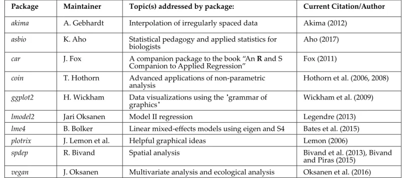
Aside from distributed and recommended packages, there are a large number of user-deined contributed pack -ages that are useful to biologists and biometrists (> 10000 as of 9/5/2017). Table 3 lists a few. Contributed R
packages can be downloaded from CRAN (the Comprehensive R Archive Network). To do this, one can go to Packages>Install package(s) on the R-GUI toolbar, and choose a nearby CRAN mirror site to minimize down-load time (non-Unix only). Once a mirror site is selected, the packages available at the site will appear. One can simply click on the desired packages to install them. Packages can also be downloaded directly from the com-mand line. To install the package vegan(Table 3),I would simply type:
install.packages("vegan")
Of course, both of these approaches require that your computer has web access. If local web access is not avail-able, libraries can be saved from the CRAN website or some other source as compressed (.zip, .tar) iles which can then be placed manually on a workstation by inserting the package iles into the “library” folder within the top level R directory,or into a path-deined R library folder in a user directory. This package can then be loaded for a particular session.
the package using the load function. For instance, to load the vegan package I would type.
load(vegan)
Or one could go to Packages>Load package(s) on the R-GUI toolbar (non-Unix only) Notwithstanding user modiication, none of packages in Table 1 require loading, as they will be loaded automatically upon opening R. Typing search() lets one see all the atached (loaded) packages (and other atached objects) currently avail -able in a work session.
Table 2 "Recommended" R packages.
Package Maintainer Topic(s) addressed by package: Current Citation/Author
KernSmooth B. Ripley Functions for kernel smoothing (and density
estimation) Wand (2015)
MASS B. Ripley Wide variety of important statistical
methods. Venables and Ripley (2002)
Matrix M. Maechler Classes and methods and operations for
matrices using 'LAPACK' and 'SuiteSparse' Bates and Maechler (2016) boot B. Ripley Bootstrapping and analytical extensions Canty and Ripley (2016),
Davison and Hinkley (1997)
class B. Ripley Functions for classiication Venables and Ripley (2002) cluster M. Maechler Functions for cluster analysis Maechler et al. (2016) codetools S. Wood Code analysis tools Tierney (2016) foreign R core team Functions for reading and writing data
stored by non-R statistical software, e.g. SAS R Core Team (2016) latice D. Sarkar Latice graphics, an implementation of
Trellis graphics functions Sarkar (2008)
mgcv S. Wood Generalized Additive Models (GAMS) Wood (2011)
nlme R core team Linear and non-linear mixed efect models Pinheiro et al. (2016) nnet B. Ripley Software for “feed-forward neural
networks” Venables and Ripley (2002)
rpart B. Ripley Recursive PARTitioning and regression trees Venables and Ripley (2002) spatial B. Ripley Functions for kriging and point patern
analysis Venables and Ripley (2002)
survival T. M. Therneau Functions for survival analysis, including penalized likelihood
Therneau (2015)
As noted in § 3, once a package is installed information its functions can be accessed using help. For example, information about the vegan package can be accessed by typing help(package= "vegan").
Given web access, newer (updated) versions of packages can be obtained using the command:
update.packages()
Note, however, that this will only give you the latest possible package applicable to the version of R that you are running. Acquiring the “very latest” version of a package may require downloading the latest version of R
detach(package:vegan)
Aside from CRAN, there are currently two large repositories of R packages. First, the bioconductor project (htp://www.bioconductor.org/packages/release/Software/html) contains a large number of packages for ge-nomic analysis (1,383 as of Sept 2017) that are not found at CRAN. Packages can be downloaded from biocon-ductor using an R script called biocLite. To download the package rRytoscape from biocondctor I would type:
source("http://bioconductor.org/biocLite.R") biocLite("RCytoscape")
Second, R-forge (htp://r-forge.r-project.org/) contains alpha releases of packages that have not yet been imple-mented into CRAN, and other miscellaneous code. Either of these sources can be speciied from Packages>Select Repositories in the R-GUI (non-Unix only)11.
Table 3 Additional, contributed R packages that may be useful to biologists and biometricians. Package Maintainer Topic(s) addressed by package: Current Citation/Author
akima A. Gebhardt Interpolation of irregularly spaced data Akima (2012)
asbio K. Aho Statistical pedagogy and applied statistics for
biologists Aho (2017)
car J. Fox A companion package to the book “An R and S
Companion to Applied Regression” Fox (2011)
coin T. Hothorn Advanced applications of non-parametric
analysis Hothorn et al. (2006, 2008)
ggplot2 H. Wickham Data visualizations using the "grammar of
graphics" Wickham et al. (2009)
lmodel2 Jari Oksanen Model II regression Legendre (2013) lme4 B. Bolker Linear mixed-efects models using eigen and S4 Bates et al. (2015) plotrix J. Lemon et al. Helpful graphical ideas Lemon (2006)
spdep R. Bivand Spatial analysis Bivand et al. (2013), Bivand and Piras (2015)
vegan J. Oksanen Multivariate analysis and ecological analysis Oksanen et al. (2016)
7�1
Datasets in packages
At this point it would be helpful to have a dataset to play with. The command: data(package = "base") lets us see all of the datasets available in the R base package while the command: data() lets us see all the datasets available within all the packages loaded onto a particular computer workstation. We will learn how to enter our own data into R shortly.
11I do not encourage downloading all of the R packages that have been developed for analysis of biological data, much
less trying out all of their functions. It is remarkable, however, to consider the range of topics these packages encompass. There are R packages for bioinformatics including packages devoted only to phylogenetics (e.g. packages ouch, picante, apTreeshape) or compiling amino acid sequences (package: seqinr)� There are libraries that allow interpolation with geo-graphic information system software (e.g. GRASS), packages speciically created for animal tracking data (adehabitat),
functions for inding spatial paterns in cells (applications in package spatstat), and even algorithms for quantifying the existence of indicator species using count data from benthic environments (package bio.infer), or discerning the efect of
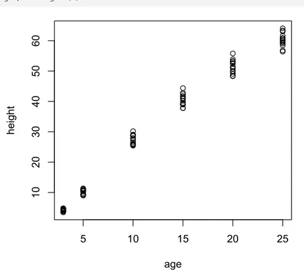
|| Example 3 -- A brief R session
The dataset Loblolly in the base package describes the height and age of loblolly pine trees (Pinus taeda), a commercially important species in the southeastern United States. To make the dataset avail-able, we type:
data(Loblolly)
We can then type: Loblolly to look at the entire dataset.
Loblolly
height age Seed 1 4.51 3 301 15 10.89 5 301 29 28.72 10 301 43 41.74 15 301 57 52.70 20 301 71 60.92 25 301 ……… 70 49.12 20 331 84 59.49 25 331
We can type head(Loblolly) To view just the irst few lines of data:
head(Loblolly) height age Seed 1 4.51 3 301 15 10.89 5 301 29 28.72 10 301 43 41.74 15 301 57 52.70 20 301 71 60.92 25 301
Because the name Loblolly is rather diicult to type, we can use the assignment operator to call the dataset something else. To assign Loblolly the name lp I simply type:
lp <- Loblolly
Note that Loblolly still exists, lp is just a copy.
Typing:
summary(lp)
summary(lp)
height age Seed Min. : 3.46 Min. : 3.0 329 : 6 1st Qu.:10.47 1st Qu.: 5.0 327 : 6 Median :34.00 Median :12.5 325 : 6 Mean :32.36 Mean :13.0 307 : 6 3rd Qu.:51.36 3rd Qu.:20.0 331 : 6 Max. :64.10 Max. :25.0 311 : 6 (Other):48
8
R and spreadsheets
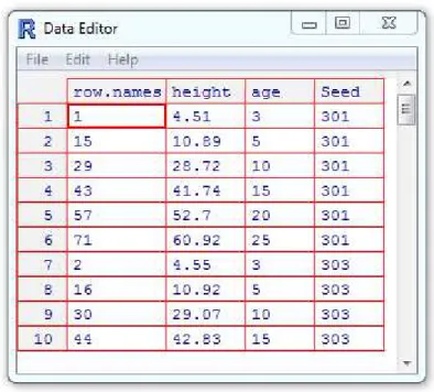
A data editor is provided by typing ix(x), when x is a dataframe or matrix (see § 10 for information on these object classes). For instance, the command ix(lp) will open the Loblolly pine dataset in the R data editor (Fig-ure 4). When x is a function or character string, then ix(x) opens a script editor containing x.
The data editor has limited lexibility compared to software whose interface is a worksheet, and whose primary purpose is data entry and manipulation, e.g., Microsoft Excel®. However, it is possible to access R from Excel® (and vice versa) through use of the RExcel package (see Heiberger and Nuewirth 2009).
Changes made to an object using ix will only be maintained for the current work session. They will not perma-nently alter objects brought in remotely to a session.
Figure 4 The irst ten observations from the Lobolly dataset in an editable spreadsheet.
8�1
attach
and
detach
The function attach will let R recognize the column names of a dataframe (more on what a dataframe is later). For instance, typing:
attach(lp)
will let R recognize the individual columns in lp (a dataframe) by name. The function detach is the program-ming inverse of attach. For instance, typing:
detach(Loblolly)
8�2
with
A safer alternative to attach is the function with. Using with eliminates concerns about multiple variables with the same name becoming mixed up in functions. This is because the variable names for a dataframe speci-ied in with will not be permanently atached in an R-session. For instance, try:
detatch(lp)
with(lp, age + height)
8�3
remove
and
rm
Typing:
remove(Loblolly)
or
rm(Loblolly)
will remove Loblolly completely from a work session. Happily, the object Loblolly (a dataset in the package datasets) cannot actually be destroyed/deleted using rm or remove (or any other commands) at the R-console.
8�4
Cleaning up
By now we can see that the R-console can quickly become clutered and confusing. To remove cluter on the
console (without actually geting rid of any of the objects in a session) press Ctrl+L or using the Edit pulldown menu to click on “Clear console”12 (non-Unix only). To remove all objects in the current session, including saved objects brought in from the working directory, one can type:
rm(list = ls(all = TRUE))
Of course, one should never include this or other equivalent lines of code in a distributed function, since it would cause users to delete their work.
12Many other keyboard shortcuts for R are available including Ctrl+U which deletes all the text from the current line, and
9 R
graphics
A strong feature of R is its capacity to create publication-quality graphs with tremendous user lexibility. The
conventional workhorse of R-graphics is the function plot. These examples in this section present just a few R graphical ideas. An extensive discussion of R graphics is given in Murrell (2005). For additional demonstra-tions go to my personal webpage htps://sites.google.com/a/isu.edu/aho/or the book website htp://www2.cose.isu. edu/~ahoken/book/.
9�1
plot
The function plot allows representation of objects deined with respect to Cartesian coordinates. It has only two required arguments.
• x deines the x-coordinate values. • y deines the y-coordinate values.
Important optional arguments include the following:
• pch speciies the symbol type(s), i.e., the ploting character(s) to be used. • col deines the color(s) to be used with the symbols.
• cex deines the size (character expansion) of the plot symbols and text. • xlab and ylab allow the user to specify the x and y-axis labels.
• type allows the user to deine the type of graph to be drawn. Possible types are "p" for points (the default),
"l" for lines, "b" for both, "c" for the lines part alone of "b", "o" for overploted, "h" for ‘histogram’ like
vertical lines, "s" for stair steps, and "n" for no ploting. Note that the command box() will also place a box around the ploting region.
We can see some symbol and color alternatives for R-plots in Figure 5.
●
●
●
5 10 15 20
5
1
0
1
5
2
0
Color number
Symb
o
l
n
u
mb
e
r
Figure 5 Some symbol and color ploting possibilities.
In the code above the x and y coordinates are both sequences of numbers from 1 to 20 obtained from the com-mand 1:20. I varied symbol colors and ploting characters (col and pch respectively) using 1:20 as well. The combination col = 1 and pch = 1 results in a black open circle, whereas the combination col = 20, pch
= 20 results in a blue illed circle. Note that we need to enclose the axis names in quotations for R to recognize
them as text. Symbol numbers 21-26 allow background color speciication using the argument bg. Many other symbol types are also possible including thousands of unicode options.
An enormous number of color choices for plots are possible and these can be speciied in at least six diferent ways. First, we can specify colors with integers as I did in Figure 5. Additional varieties can be obtained by drawing numbers colors()[number] (Figure 6).
e <- expand.grid(1:20, 1:32)
plot(e[,1], e[,2], bg = colors()[1:640], pch = 22, cex = 2.5, xaxt = "n", yaxt = "n", xlab = "", ylab = "")
1 2 3 4 5 6 7 8 9 10 11 12 13 14 15 16 17 18 19 20
21 22 23 24 25 26 27 28 29 30 31 32 33 34 35 36 37 38 39 40
41 42 43 44 45 46 47 48 49 50 51 52 53 54 55 56 57 58 59 60
61 62 63 64 65 66 67 68 69 70 71 72 73 74 75 76 77 78 79 80
81 82 83 84 85 86 87 88 89 90 91 92 93 94 95 96 97 98 99 100
101 102 103 104 105 106 107 108 109 110 111 112 113 114 115 116 117 118 119 120
121 122 123 124 125 126 127 128 129 130 131 132 133 134 135 136 137 138 139 140
141 142 143 144 145 146 147 148 149 150 151 152 153 154 155 156 157 158 159 160
161 162 163 164 165 166 167 168 169 170 171 172 173 174 175 176 177 178 179 180
181 182 183 184 185 186 187 188 189 190 191 192 193 194 195 196 197 198 199 200
201 202 203 204 205 206 207 208 209 210 211 212 213 214 215 216 217 218 219 220
221 222 223 224 225 226 227 228 229 230 231 232 233 234 235 236 237 238 239 240
241 242 243 244 245 246 247 248 249 250 251 252 253 254 255 256 257 258 259 260
261 262 263 264 265 266 267 268 269 270 271 272 273 274 275 276 277 278 279 280
281 282 283 284 285 286 287 288 289 290 291 292 293 294 295 296 297 298 299 300
301 302 303 304 305 306 307 308 309 310 311 312 313 314 315 316 317 318 319 320
321 322 323 324 325 326 327 328 329 330 331 332 333 334 335 336 337 338 339 340
341 342 343 344 345 346 347 348 349 350 351 352 353 354 355 356 357 358 359 360
361 362 363 364 365 366 367 368 369 370 371 372 373 374 375 376 377 378 379 380
381 382 383 384 385 386 387 388 389 390 391 392 393 394 395 396 397 398 399 400
401 402 403 404 405 406 407 408 409 410 411 412 413 414 415 416 417 418 419 420
421 422 423 424 425 426 427 428 429 430 431 432 433 434 435 436 437 438 439 440
441 442 443 444 445 446 447 448 449 450 451 452 453 454 455 456 457 458 459 460
461 462 463 464 465 466 467 468 469 470 471 472 473 474 475 476 477 478 479 480
481 482 483 484 485 486 487 488 489 490 491 492 493 494 495 496 497 498 499 500
501 502 503 504 505 506 507 508 509 510 511 512 513 514 515 516 517 518 519 520
521 522 523 524 525 526 527 528 529 530 531 532 533 534 535 536 537 538 539 540
541 542 543 544 545 546 547 548 549 550 551 552 553 554 555 556 557 558 559 560
561 562 563 564 565 566 567 568 569 570 571 572 573 574 575 576 577 578 579 580
581 582 583 584 585 586 587 588 589 590 591 592 593 594 595 596 597 598 599 600
601 602 603 604 605 606 607 608 609 610 611 612 613 614 615 616 617 618 619 620
621 622 623 624 625 626 627 628 629 630 631 632 633 634 635 636 637 638 639 640
Figure 6 Color choices from colors().
Second, we can specify colors using actual color names, e.g. "white", "red", "yellow". For a visual dis-play of essentially all the available named colors in R type: example(colors).
Third, we can deine colors by requesting red green and blue color intensities with the function rgb. Usable light intensities can be made to vary individually from 0 to 255 (i.e., within an 8 bit format). Fourth, we can specify colors using the function hcl which controls hues, chroma, and luminescence and transparency. Fifth, we can deine colors using hexadecimal codes13, e.g., blue = #0000FF. Finally we can specify colors using entirely
diferent paletes. Figure 7 shows six pie plots. Each pie plot uses a diferent color palete. Each pie slice from each pie represents a distinct segment of the palete.
Fig.7() # See Appendix code
13A data coding system that uses 16 symbols: the numbers 1-9, and the letters A-F. Hexadecimals are primarily used to provide a more
1 2 3 4 5 6 7 8 9 10 11 12 Rainbow colors 1 2 3 4 5 6 7 8 9 10 11 12 Heat colors 1 2 3 4 5 6 7 8 9 10 11 12 Topographic colors 1 2 3 4 5 6 7 8 9 10 11 12 Gray colors 1 2 3 4 5 6 7 8 9 10 11 12
Colors using hcl arguments 1
1 2 3 4 5 6 7 8 9 10 11 12
Colors using hcl arguments 2
Figure 7 Use of color paletes in R. Note that the numbers do not correspond to actual color type designations.
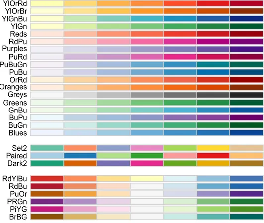
A large number of additional paletes (including color-blind-safe paletes) can be obtained using the R-package RColorBrewer.
BrBGPiYG PRGn PuOr RdBu RdYlBu Dark2 PairedSet2 Blues BuGn BuPu GnBu Greens Greys OrangesOrRd PuBu PuBuGn PuRd PurplesRdPu RedsYlGn YlGnBuYlOrBr YlOrRd
Figure 8 RColorBrewer color-blind-safe seven category paletes. Top paletes are so-called "sequential" paletes, middle paletes are "qualitative", and botom paletes are "divergent".
Here are the hexadecimal names for the "Set2" palette chunks in Figure 8.
brewer.pal(7,"Set2")