Braz. J. Phys. vol.36 número2A

Brazilian Journal of Physics, vol. 36, no. 2A, June, 2006 401

Electronic Transport Through a Single-Wall Carbon Nanotube

with a Magnetic Impurity

T. Lobo∗, M. S. Figueira∗, and M. S. Ferreira†

∗_{Departamento de F´ısica, Universidade Federal Fluminense Av. Litorˆanea s/n, 24210-346 Niter´oi-RJ, Brazil and}

†_{Physics Department, Trinity College, Dublin 2, Ireland}

Received on 4 April, 2005

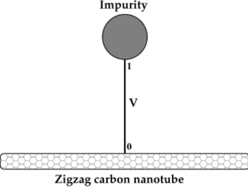
We are interested in studying the transport properties of metallic single-wall carbon nanotubes (SWCNTs) with isolated magnetic impurities. We consider a metallic zigzag SWCNT in the form of an infinitely long cylinder of diameterD, connected by two metallic electrodes under a bias voltageE_{, with a magnetic impurity} located on its surface. To describe the Kondo resonance we employ an impurity version of the atomic model, previously developed to study the Kondo insulator properties in the lattice case. We calculate the approximate Green’s functions of the impurity Anderson model by employing the exact solution of the atomic limit of the Anderson model, where we use the completeness condition to choose the position of the chemical potential. We consider the SWCNT Green’s functions in a tight-binding approach. We calculate density of states curves that characterize well the structure of the Kondo peak and we also present the dependence of the conductance with the diameter of the SWCNT.

Keywords: Transport properties; Single-wall carbon nanotubes; Magnetic impurities

I. THE ZIGZAG SINGLE-WALL CARBON NANOTUBE

A single-wall carbon nanotube (SWCNT) can be described as a graphene sheet rolled into a cylindrical shape so that the structure is one-dimensional with axial symmetry. Depend-ing on their chirality, that can be expressed by the real space unit vectorsa~1anda~2of the hexagonal lattice, the SWCNT vary from being metallic ( see Fig. 2) to semi-conducting (see Fig. 3). In this paper we are interested in studying zigzag SW-CNT’s that correspond to the chiral vectors(n,0), wherenis an integer proportional to the diameterDof the nanotube [1]. The zigzag SWCNT is always metallic whennis a multiple of 3 and the energy dispersion relationEqa(k)for the zigzag

nanotube can be written as [1]

E_qa(k) =±γ0

(

1±4cos

Ã√

3ka 2

!

cosq˜+4cos2q˜

)1₂

, (1)

with³−√π

3<ka< π √ 3

´

,(q=1, ...,2n), where ˜q= q_nπ and the hopping energy between the carbon atoms of the nanotube, γ0, is considered as≈2.7 eV.

V

✁ ✁ ✁ ✁ ✁ ✁ ✁ ✁ ✁ ✁ ✁ ✁ ✁ ✁ ✁ ✁ ✁ ✁ ✁ ✁ ✁ ✁ ✁ ✁ ✁ ✁ ✁ ✁ ✁ ✁ ✁ ✁ ✁ ✁ ✁ ✁ ✁ ✁ ✁ ✁ ✁ ✁ ✁ ✁ ✁ ✁ ✁ ✁ ✁ ✁ ✁ ✁ ✁ ✁ ✁ ✁ ✁ ✁ ✁ ✁ ✁ ✁ ✁ ✁ ✁ ✁

Zigzag carbon nanotube Impurity

1

0

FIG. 1. Pictorial view of the zigzag SWCNT with an impurity at-tached on its surface,V is the hybridization between the SWCNT conduction band and the localized impurity level.

II. CONDUCTANCE OF A ZIGZAG SWCNT

The Kondo effect explains the enhancement of the low-temperature resistivity shown by a metal with magnetic im-purities at low temperatures. The Kondo effect was experi-mentally detected in quantum dots [2] and in carbon nanotube devices [3]. These systems can be modeled by the Ander-son impurity model and in this paper we employ an impurity version of the atomic model, previously applied to study the Kondo insulators [8], to describe the electronic transport prop-erties of zigzag SWCNT’s. In Fig. 1 we represent a pictorial view of the zigzag SWCNT with an impurity laterally attached [4]. At low temperatures and bias voltage, electron transport is coherent and a linear-response conductance is given by the Landauer-type formula [5]

G=2e 2

~

Z µ

−∂n_∂ωF

¶

S(ω)dω, (2)

wherenF is the Fermi function andS(ω)is the transmission

probability of an electron with energy~ω_{. This probability is} given byS(ω) =Γ2_|Gσ

00|2, whereΓcorresponds to the cou-pling strength of the site0of the SWCNT conduction band to the impurity, here represented by the site1, which is pro-portional to the kinetic energy of the electrons in the zigzag SWCNT. The Green functionGσ₀₀ can be rewritten in terms of the exact Green function of the impurity,Gσ_imp, calculated by the Dyson equation withV_{=|0iVh1|+|1iVh0|being the} hybridization. The dressed Green’s functions at the site0can be written in terms of the undressed Green’s functions local-ized at the impurity,g11, and the undressed Green’s functions of the conduction band,g00

Gσ00=gσ00+gσ00V Gσ10+gσ01V Gσ00, (3)

402 T. Lobo et al.

Solving the equation system above and consideringg10=0 andg01=0, we can write

Gσ00=

gσ₀₀ (1−gσ₀₀V2_gσ

11)

, (5)

wheregσ₀₀is given by [1]

gσ_{j j}′=

i 2nγ02

∑

Eeikx(xj−xj′)_e

2πi j

³

y j−y_j′

´

na

cos³j_nπ´sin³kxa√3

2

´ (6)

andkxobeys the relation

cos

Ã

kxa

√ 3 2

!

=

z2

γ02−1−4cos2

³

jπ

n

´

4cos³j_nπ´

(7)

and

gσ₁₁=M₂at_,σ(z). (8) whereMat_2,σ(z)is calculated in Sec. IV.

-4 -2 0 2 4

ω 0

0.5 1

ρc

n=9

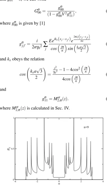
FIG. 2. Density of states per unit cell of the conduction band of the nanotube(9,0)which presents metallic behavior. The chemical potential is located atµ=0 in all the density of states figures.

-4 -2 0 2 4

ω 0

0.5 1

ρc

n=11

FIG. 3. Density of states per unit cell of the conduction band of the nanotube(11,0)which presents semiconducting behavior.

III. THE ANDERSON IMPURITY MODEL

The Hamiltonian for the Anderson impurity with infinite Coulomb repulsionUis given by

H =

∑

k,σ

Ek,σc†k,σck,σ+

∑

σ Ef,σXf,σσ

+V

∑

k,σ ³

X†_f,0σck,σ+c†k,σXf,0σ

´

, (9)

where the first term represents the conduction electrons (c -electrons), the second describes the Anderson impurity char-acterized by a localized f level Ef,σ, (we employ the f

let-ter to indicate localized electrons at the impurity site) and the last one corresponds to the interaction between the c -electrons and the impurity. For simplicity we consider a con-stant hybridizationV. We employ the Hubbard operators [6] to project out the double occupation state |f,2i, from the local states on the impurity. The identity decomposition in the reduced space of local states at the impurity is given by Xf,00+Xf,σσ+Xf,σσ=I, whereσ=−σ, and the threeXf,aa

are the projectors into the states|f,ai. The occupation num-bers on the impuritynf,a=<Xf,aa>should then satisfy the

“completeness” relation

nf,0+nf,σ+nf,σ=1. (10)

IV. THE ATOMIC MODEL

To obtain the exact f Green function Gf f,σ(ji,z) in real

space for the impurity at siteji, one can follow a procedure

similar to the one used in [7] within the chain approximation, but considering all the possible cumulants in the expansion as it was done in [8] for the Anderson lattice. As with the Feyn-mann diagrams, one can rearrange all those that contribute to the exact Gf f,σ(ji,z) by defining an effective cumulant

M₂e f f_,σ(ji,z), that is given by all the diagrams ofGf f,σ(ji,z)that

can not be separated by cutting a single edge (usually called “proper” or “irreducible” diagrams). We shall consider that the impurity is at the origin, and drop the indexjifrom all the

quantities. The exact GFGf f,σ(z)is then given by replacing

the bare cumulantM0

2,σ(z) =−D0σ/(z−εf), whereD0σ=<<

Xf,00+Xf,σσ >>o, by the effective cumulantM2e f f,σ(z)at all

the filled vertices of the chain diagrams in [7].The exact GF for the f electron is then written as

Gf f,σ(z) = M

e f f

2,σ(z)

1₋Me f f_2,σ(z)|V_|2_∑

kGoc,σ(k,z)

, (11)

whereGo

c,σ(k,z) =−1/(z−ε(k)).The exact atomic f Green

function has the same form of Eq. (11), and it is calculated exactly in the Appendix A (cf. Eq. 13), and we write

Gat_{f f,σ}(z) = M

at

2,σ(z)

1−Mat

2,σ(z)|V|2∑kGoc,σ(k,z)

Brazilian Journal of Physics, vol. 36, no. 2A, June, 2006 403

From this equation we then obtain an explicit expression for Mat_2,σ(z) in terms of Gat_{f f,σ}(z). To decrease the contribution of thec electrons, whose effect was overestimated by con-centrating them at a single energy level we shall replaceV2 by∆2, with∆=πV2_{/W is of the order of the Kondo peak’s} width, whereW is related to the nanotube hopping energy by W =6γo. The atomic approximation consists in substituting

Me f f_2,σ(z)in Eq. (11) by the approximateMat

2,σ(z)given by Eq.

(12). AsM₂at_,σ(z)iskindependent, we can easily obtain the local Green function for the Anderson impurity for the zigzag nanotube, which is given by Eq. (11) but withGoc,σ(k,z)given

by Eq. (6) and in the same way we obtain the conduction (Gc)

and mixed (Gf c) Green’s functions. One still has to decide

what value ofE0should be taken. As the most important re-gion of the conduction electrons is the Fermi energy, we shall useE0=µ−δE0, leaving the freedom of small changesδE0 to adjust the results in such way that the completeness relation given by Eq. (10) should be satisfied.

V. RESULTS AND CONCLUSIONS

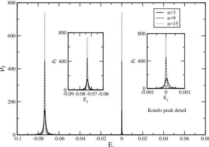
In Fig. 4 we plot the evolution of the density of states cor-responding to a Kondo situation for three representativen val-ues. We can see the two structures characteristic of the Kondo densities of states. One non-resonant peak located at theEf

position and the Kondo peak located at the chemical potential µ=0. In the insets we represent details of each structure.

-0.1 -0.08 -0.06 -0.04 -0.02 0 0.02 0.04 0.06 0.08

E_f 0

200 400 600 800

ρf

n=3 n=9 n=15

-0.001 0 0.001

Ef 0 400 800

ρf

-0.09 -0.08 -0.07 -0.06 Ef 0 400 800

ρf

Kondo peak detail

FIG. 4. Density of states of the impurity f-electrons forT =0.01∆, with∆=0.01. In the left inset we present a detail of the non-resonant structure located at around Ef =−0.08 and in the right inset we present a detail of the Kondo peak located atµ=0.

In Fig. 5 we represent the conductance of a side-coupled impurity in the zigzag nanotube. The Kondo effect depends on the diameter of the SWCNT and change the conductance of the system. The conductance varies more than two orders of magnitude as the nanotube diameter parameternincreases. At the same time, the Kondo peak becomes more steep,

indi-cating that the Kondo temperature decreases as can be seen in the right inset of Fig. 4.

3 6 9 12 15 18 21 24 27 30 33 36

n 0.01

0.1 1 10

G/G

0

(Arbitrary units)

T=0.0001∆ Ef=-7∆ ∆=0.01

FIG. 5. The normalized linear conductance as function of the nan-otube diameter, here represented by the parametern. The parameters employed are indicated in the figure.

Appendix A: Atomic solution

We assume the zero conduction bandwidthW =0. There-fore we eliminate from the Hamiltonian the hoping contribu-tions. This corresponds to consider the relationship between a given~k state of the conduction band and one localized f state. In this case the analytical solution of the Hamiltonian is known [8]. The f atomic Green function is given by

Gat(ω) =eβΩ 8

∑

i=1

mi

ω−ui

, (13)

whereΩis the thermodynamical potential and the poles of the Green’s functions are given by

u1=E3−E1=E8−E5=E7−E4= 1

2(εq+εf−∆); (14)

u2=E5−E1=E8−E3=E7−E2= 1

2(εq+εf+∆); (15)

u3=E12−E10= 1

2

¡ε

q+εf−∆′¢; (16)

u4=E12−E9= 1

2

¡_ε

q+εf+∆′¢; (17)

u5=E9−E2=εq−

1

2

¡∆_′

−∆¢

; (18)

u6=E10−E2=εq+

1

2

¡_∆′

+∆¢

; (19)

u7=E9−E4=εq−

1

2

¡∆_′+∆¢

404 T. Lobo et al.

u8=E10−E4=εq+

1

2

¡_∆′

−∆¢

, (21)

where the residues are

m1=cos2φ[1+e− 1

2β(εf+εq−∆)₊

3

2e −1

2β(εf+εq+∆)₊3

2e

−β(εf+εq_{)]; (22)}

m2=sin2φ[1+e− 1

2β(εf+εq+∆)

+3

2e

−12β(εf+εq−∆)₊3

2e

−β(εf+εq_{)]; (23)}

m3=cos2λ[e− 1

2β(εf+3εq+∆′)_+e−12β(εf+2εq)_{]; (24)}

m4=sin2λ[e− 1

2β(εf+3εq−∆′)_+e−12β(εf+2εq)_{]; (25)}

m5= 1

2sin 2_φ

cos2λ[e−12β(εf+εq−∆)_+e−12β(εf+3εq−∆′)_{]; (26)}

m6= 1

2sin 2_φ

sin2λ[e−12β(εf+εq−∆)_+e−12β(εf+3εq+∆′)_{]; (27)}

m7= 1

2cos

2_φcos2_λ[e−1

2β(εf+εq+∆)_+e−21β(εf+3εq−∆′)_{]; (28)}

m8= 1

2cos

2_φsin2_λ[e−1

2β(εf+εq+∆)_+e−21β(εf+3εq+∆′)_{], (29)}

where ∆ =

q

(εq−εf)2+4V2, ∆′ =

q

(εq−εf)2+8V2,

tanφ=_(ε 2V

q−εf+∆) and tanλ=

2√2V (εq−εf+∆′).

[1] R. Saito, G. Dresselhaus, and M. S. Dresselhaus,Physical Prop-erties of Carbon Nanotubes, Imperial College Press, (1999).

[2] D. Goldhaber-Gordon, Hadas Shtrikman, D. Mahalu, David Abusch-Magder, U. Meirav, and M. A. Kastner, Nature391, 156 (1998).

[3] Jesper Nygard, David Henry Cobden, and Paul Erik Lindelof, Nature408, 342 (2000).

[4] R. Franco, M. S. Figueira, and E. V. Anda, Phys. Rev. B67, 155301 (2003).

[5] K. C. Kang, S. Y. Cho, J. J. Kim, and S. C. Shin, Phys. Rev. B.

63, 113304 (2001).

[6] M. S. Figueira, M. E. Foglio, and G. G. Martinez, Phys. Rev. B

50, 17933 (1994).

[7] R. Franco, M. S. Figueira, and M. E. Foglio, Phys. Rev. B66, 45112 (2002).