!""#$ #%!""&$ ' $ #
( )* + ,
-&!".!%/0" $ -,$ # 1
2
( )* + ,
-&!".!%/0" $ -,$ # 1
2
!""#$ #%!""&$ ' $ #
!
"
!
#
This paper applies recent advances in both modeling and control of Linear Parameter-Varying (LPV) systems to a vibroacoustic setup whose dynamics is highly sensitive to variations in the temperature. Based on experimental data, an LPV model is derived for this system using the State-space Model Interpolation of Local Estimates (SMILE) technique. This modeling technique interpolates linear time-invariant models estimated at distinct operating conditions of the system (in this case, different temperatures). Using the obtained LPV model, gain-scheduled and robust multiobjective H2/H∞ state feedback
controllers are designed such that can consider a priori known bounds on the rate of parameter variation. Numerical simulations using the closed-loop systems are performed to validate the controllers and to show the advantages and versatility of the proposed techniques.
Keywords: Gain-scheduled and robust control, LPV modeling, H2 and H∞ performance,
linear parameter-varying systems
Introduction
*
A main source of noise within aircraft cabins is the vibration of the surrounding structure, usually denoted as structural noise (Berglund et al., 1996; Persson and Björkman, 1988). Research in the area of acoustics has shown that active control strategies are efficient in reducing this noise in the low frequency range (see, for example, Alujevic et al., 2008; Camino and Arruda, 2009; Donadon et al., 2006; Fuller and von Flotow, 1995; Kaiser et al., 2003; Meurers et al., 2002; Sas et al., 1995). Several of these techniques assume that the plant under consideration is linear time-invariant (LTI), although this is not a realistic assumption for some applications. For instance, aircraft structures are frequently subjected to temperature variations that cause significant changes in its dynamics. To use robust control synthesis techniques for such parameter-varying systems, the nominal model and the uncertainty bounds should be appropriately determined, to ensure a realistic trade-off between performance and robustness. For most practical applications, however, this is a difficult task, and the estimated uncertainty set is in general too conservative. Therefore, a more elaborate control strategy should be investigated which can be used for linear parameter-varying (LPV) systems. This topic has received attention from the control community for over a decade, during which there has been a continuing effort to design LPV controllers, scheduled as a function of the varying parameters, that achieve higher performance while still guaranteeing stability for all possible parameter variations (see, for instance, Apkarian and Adams, 1998;
Paper accepted April, 2010. Technical Editor: Domingos Alves Rade.
Apkarian et al., 1995; Leith and Leithead, 2000; Packard, 1994; Rugh and Shamma, 2000; Scherer, 2001; Shamma and Athans, 1992). In the LPV control framework, the scheduling parameters that govern the variation of the dynamics of the system are usually a priori unknown, but measured or estimated in real-time (Shamma and Athans, 1991).
systems with an a priori known bound on the rate of parameter variation. The case where the system can have a homogeneous polynomial dependency on the scheduling parameter has been considered in De Caigny et al. (2009a, 2010a, 2010b).Most LPV control design techniques require an LPV model of the system that accurately describes the variation of the system dynamics over the workspace. However, while identification of linear time invariant (LTI) systems based on measured input-output (IO) data has been intensely studied and LTI model estimation algorithms are widely spread, estimation of LPV models remains a difficult problem which is still in a state of development. In the literature, there exist two main approaches to obtain LPV models: a global identification approach (see, for example, Bamieh and Giarré, 2002; Felici et al., 2007; Lee and Poolla, 1999; Nemani et al., 1995; Verdult and Verhaegen, 2005) and a local modeling approach (see, for example, De Caigny et al., 2008c, 2009b, 2011; Lovera and Mercere, 2007; Paijmans et al., 2008; Steinbuch et al., 2003; Wassink et al., 2005). The global approach is based on the assumption that it is possible to perform a global experiment by exciting the system while the scheduling parameters are persistently changing the system dynamics. In case it is impossible to perform a global experiment, it is appropriate to use a local approach, based on the interpolation of a set of local LTI models that are estimated using a collection of local experiments, performed by exciting the system at different fixed operating conditions. To properly interpolate these local models, all local LPV modeling techniques require that the local LTI models are defined with respect to a consistent state-space representation. Afterwards, an appropriate methodology is applied to construct an LPV model that interpolates these consistent local models. The main drawback of the local approach is the fact that the time propagation of the scheduling parameter is not used. Therefore, these local methods are more suitable for systems with scheduling parameters that vary slowly in time; a common guideline in interpolating gain-scheduling control practice (Shamma and Athans, 1992).
The aim of this paper is to show the recent advances in both modeling and control of LPV systems using a vibroacoustic setup as a practical application. First, experimental data is used to obtain an LPV model of the vibroacoustic setup using the State-Space Model Interpolation of Local Estimates (SMILE) technique; a local LPV modeling technique developed in De Caigny et al. (2008c, 2009b). Second, using the obtained LPV model, multiobjective H2/H∞ gain-scheduled and robust static state feedback controllers are computed. The LPV control design is then validated through numerical simulations. Finally, the advantages and disadvantages of the proposed LPV modeling and control design techniques are discussed. The paper is organized as follows. In the next section, the vibroacoustic application is introduced. The following section starts by presenting an overview of the SMILE technique which is then used to obtain an LPV model of the vibroacoustic setup. The synthesis conditions for gain-scheduled and robust H2 and H∞ state feedback control which are applied to the obtained LPV model is then presented as well as the concluding remarks.
Vibroacoustic Application
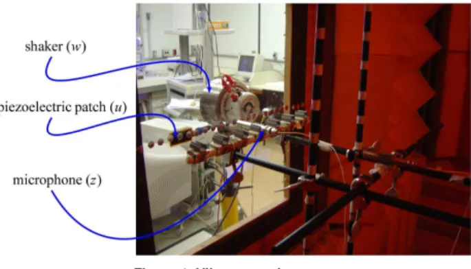
This section describes the vibroacoustic setup (displayed in Fig. 1), that consists of a lexan plate clamped on a rigid baffle in a semi-anechoic room (see Donadon et al., 2006, for details). The exogenous disturbance w that causes the vibration of the plate is provided by a point force driven by a shaker. The control input u, used to attenuate the sound pressure inside the semi-anechoic room, is provided by a flexural moment driven by a piezoelectric patch attached to the plate. The output z is the sound pressure measured by a single microphone, located in the semi-anechoic room near the plate.
Figure 1. Vibroacoustic setup.
The experiments performed by the authors in Donadon et al. (2006) revealed that the system dynamics was highly sensitive to the temperature in the semi-anechoic room. Therefore, the setup is an LPV system with the temperature as the scheduling parameter. For the modeling of this vibroacoustic setup, it is necessary to consider a local LPV modeling approach because of the slow rate of variation of the temperature. Indeed, since the temperature can only be changed slowly, a long measurement should have to be performed to ensure the conditions of persistent excitation of the scheduling parameter (Bamieh and Giarré, 2002), resulting in an intractable amount of data. Therefore, performing local identification experiments, for different fixed values of the temperature, is the most convenient option.
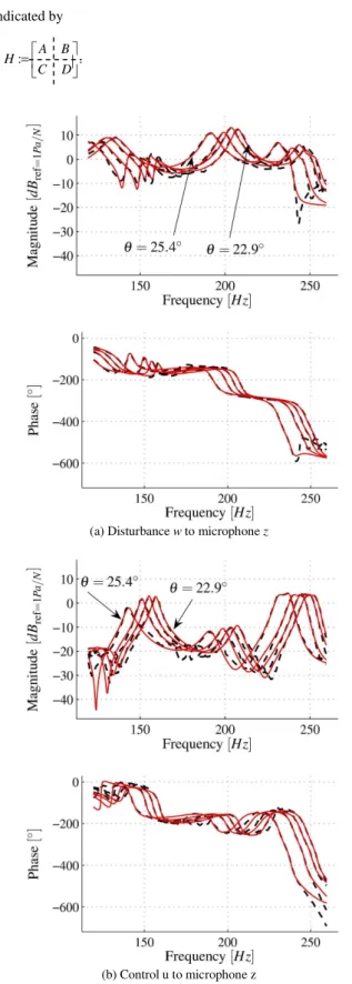
To apply the local approach, frequency response functions (FRFs) were measured from the disturbance w and the control input
u to the output z at four different temperatures θ ∈{22.9°, 23.4°, 24.4°, 25.4°}. Based on the measured FRFs, a 10th-order discrete-time state-space LTI model has been estimated at each operating condition, using the subspace identification method (Ljung, 1999; van Overschee and Moor, 1996; Verhaegen, 1994) implemented in the Matlab Identification toolbox. Figure 2 presents the magnitude and phase of the experimentally obtained FRFs (dashed) and of the corresponding estimated LTI models (solid) in the frequency range 120 – 260 Hz. All the estimated models have five complex poles, for instance, the poles of the estimated model from w to z
corresponding to the temperature 22.9º are located at 135 Hz, 160 Hz, 206 Hz, 247 Hz, and 253 Hz. The LTI models clearly show a good correspondence to the FRFs. The next section shows how to use the SMILE technique to obtain an LPV model by interpolating these four LTI models. Notice that the output sound pressure z is given by z = Hu(jω)u + Hw(jω)w, where Hw(jω) and Hu(jω) denote respectively the transfer functions from the disturbance w and the control input u to the output z. In the active noise control community, Hw(jω) is referred as the primary source and Hu(jω) as the secondary source.
LPV Modeling Using the Smile Technique
This section presents how to use the SMILE technique to model the vibroacoustic setup. For a detailed presentation, see De Caigny et al. (2008c). The notation in this section is as follows: matrices associated with the interpolating LPV model are denoted using standard math font, e.g., A0, …; matrices associated with the local LTI models are denoted using San Serif font, e.g., Aℓ, …; the
subscript ℓ indicates the index of the local model. Throughout the
paper, the discrete-time state-space model
(
)
( )
( )
( )
( )
( )
1
: x k Ax k Bu k
H
z k Cx k Du k
+ = +
=
= +
is indicated by
: .
A B
H
C D
=
(a) Disturbance w to microphone z
(b) Control u to microphone z
Figure 2. Measured FRFs (black, dashed line) and estimated 10th
-order LTI models (red, solid line) for θθθθ∈∈∈∈ {22.9º, 23.4º, 24.4º, 25.4º}.
The interpolating LPV model is chosen to have the following state-space representation affine in the single scheduling parameter
θ∈ :
( )
0 1 0 10 1 0 1
: ,
A A B B
H
C C D D
θ
θ
θ
θ
θ
+ +
=
+ +
(1)
where
A0, A1∈ n×n, B0, B1∈ n×r, C0, C1∈ s×n, and D0, D1∈ s×r.
This choice has the advantage that the LPV model H(θ) given by model (1) can be used in LPV control synthesis techniques for affine LPV models (for example, Amato et al., 2005; Apkarian et al., 1995; de Souza and Trofino, 2006; Lu et al., 2008) as well as in the linear fractional transformation framework (for example, Packard, 1994; Scherer, 2001). Moreover, when θ is bounded, model (1) can be converted exactly in a polytopic LPV model1 with two vertices, which is useful since control synthesis for polytopic models has been widely studied (De Caigny et al., 2008a, 2008b; Leite and Peres, 2004; Montagner et al., 2007; Oliveira and Peres, 2008). The recent work De Caigny et al. (2011) has extended the LPV modeling technique to consider a more general class of LPV models that can be parameterized using a homogeneous polynomial dependency on the scheduling parameter, which include as a particular case, affine models.
The aim of the SMILE technique is to estimate the system matrices of model (1) such that the resulting LPV model H(θ) interpolates the m local LTI models
~ ~
~
~ ~
: l l , 1,..., ,
l
l l
A B
H l m
C D
= =
(2)
identified at distinct operating conditions, that is, for different
fixed values of the scheduling parameter θ , indicated by θ~ for l = 1, …, m. All local LTI models are assumed to have the same number of states n, the same number of inputs r and the same number of outputs s. As the state-space representation is not unique, the local models (2) cannot be readily interpolated since it is not guaranteed that they are represented with respect to the same state-space basis. Therefore, a similarity transformation matrix Tl needs to be calculated for each local model such that the transformed models
~ ~
-1 -1
~ ~
:
1,...,
l l
l l l l l
l
l l
l l l
A B T A T T B
H
C D
C T D
l m
= =
=
(3)
are defined with respect to a consistent state-space representation. Once the models (3) have been calculated, an optimization problem can be formulated and solved to find the optimal system matrices of the interpolating LPV model (1). Assuming that the m MIMO LTI
models ~
l
H (2) are available, the SMILE technique consists of five steps to compute an interpolating LPV model (see the flowchart in Fig. 3).
1
Figure 3. Flowchart of the SMILE technique.
These five steps are now briefly presented and applied to the four (m = 4) local 10th-order 2-input 1-output LTI models identified for the vibroacoustic setup.
STEP 1: Choose one input-output (IO) combination (i, j) for all
original local MIMO models ~
l
H to obtain m local SISO models
( ) ( )
( ) ( )
~ ~
~ , :,
, ,
~ ~
, , , ,:
: l l j , 1,..., .
l i j
l i j l i
A B
H l m
C D
= =
For the vibroacoustic setup, the IO combination (i, j) = (1,2) from the control input u to the microphone z is chosen, thus yielding
four LTI SISO models ~
l
H , (1,2), l =1, …, 4.
STEP 2: Calculate the poles pl (independent of the choice of
IO-combination (i, j)) and zeros
( )
, 1,2
l
z of the original local SISO
models ( )
~ , 1,2
l
H . Sort these poles and zeros such that they are in the
same order for all local SISO models ( )
~ , 1,2
l
H . Fig. 4 shows the real and imaginary part of the poles and zeros of the 4 local SISO
models ( )
~ , 1,2
l
H as a function of the varying temperature θ. All local models have 5 complex conjugated pole pairs, 1 non-minimum phase real zero and 4 complex conjugated zero pairs. The sorting of the poles and zeros is indicated in Fig. 4 with solid lines that connect corresponding poles (resp. zeros) for the 4 different local temperatures.
(a) Poles l
p
Figure 4. Poles and zeros of the local models H~l,
( )
1,2 .(b) Zeros
( )
, 1,2
l z
Figure 4. (Continued).
STEP 3: Divide the local SISO models ( )
~ , 1,2
l
H into a gain
( )
, 1,2
l
K multiplied by the series connection of τ1 1st-order and τ2 2nd -order state-space submodels ( )
, 1,2
l
Hτ expressed in the observable form. Then, explicitly calculate this series connection to obtain a new and consistent state-space representation of the local SISO models (denoted as
( )
, 1,2
l
H ). Since all LTI SISO models are 10th -order, they can be represented by a gain multiplied by the series connection of τ2 = 5 2nd-order submodels. In Fig. 4 this division is emphasized by assigning the poles and zeros 5 different markers and colors: poles and zeros with the same marker and color are assigned to the same LTI SISO submodel.
STEP 4: Calculate, for each local model ( )
~ , 1,2
l
H , the similarity transformation matrix Tl that transforms the system matrices of
( )
~ , 1,2
l
H into those of
( )
, 1,2
l
H . Apply this transformation matrix
l
T
to the corresponding original MIMO LTI model ~
l
H to obtain the model
l
H .
STEP 5: To obtain the system matrices of the interpolating
MIMO LPV model (1), the following linear least-squares cost function is minimized
2 2
~ ~
0 1 0 1
1
2 2
~ ~
0 1 0 1
m
F F
F F
E A A A B B B
C C C D D D
θ θ
θ θ
=
= + − + + − +
+ + − + + −
Σ
where || ||F represents the Frobenius norm of a matrix.
(a) Disturbance w to microphone z (b) Control u to microphone z
Figure 5. The interpolating LPV model, evaluated at 11 different temperatures (black, solid with dots) compared to the 4 local LTI MIMO models (red, solid).
The quality of the fit can also be numerically verified by comparing the vector of Hankel singular values (Moore, 1981) of the local LTI models with the interpolating LPV model evaluated at the four local operating conditions. These vectors, for the LTI and the LPV case, are respectively denoted by Glti[i] and Glpv[i],
for i = 1, ..., 4. Table 1 presents the relative difference between these two vectors, calculated as ║Glti[i] −Glpv[i] ║2 / ║Glti[i] ║2.
Table 1. Relative difference between the Hankel singular values of the local LTI models and the interpolating LPV model evaluated at the 4 operating conditions.
Index i of the operating condition
Model 1 2 3 4
w → z 0.0368 0.0175 0.1005 0.0466
u → z 0.0647 0.0307 0.0665 0.0221
Gain-Scheduled and Robust H2 and H∞∞∞∞ State Feedback
This section presents synthesis procedures for gain-scheduled and robust H2 and H∞ state feedback controllers for discrete-time polytopic LPV systems with known bounds on the rate of parameter variation. First, the modeling of the uncertainty domain is introduced, then the synthesis conditions are given and afterwards state feedback controllers are computed for the LPV model obtained in the previous section. A schematic view of the closed-loop system is shown in Fig. 6, in which the model H(α) already contains the transfer functions of the primary and the secondary sources.
Figure 6. Schematic view of control configuration.
Modeling of the Uncertainty Domain
Consider the polytopic discrete-time linear parameter-varying system
( )
(
( )
)
(
( )
)
(
( )
)
( )
(
)
(
( )
)
(
( )
)
:
u
z w u
A k B k B k
H
C k D k D k
α α α
α
α α α
=
(4)
where the system matrices
A(α(k)) ∈ n×n
, Bw(α(k)) ∈ n×r
, Bu(α(k)) ∈ n×m
, Cz(α(k)) ∈ s×n
,
Dw(α(k)) ∈ s×r
, and Du(α(k)) ∈ s×m
belong to the polytope
= {(A,Bw,Bu,Cz,Dw,Du)(α(k)): (A,Bw,Bu,Cz,Dw,Du)(α(k)) =
Σ
Ni=1αi(k) (Ai,Bw,i,Bu,i,Cz,i,Dw,i,Du,i), α(k) ∈ΛN } (5)with the vector of time-varying parameters α(k) ∈ N belonging to
the unit simplex given by
ΛN = {ξ∈ N :
Σ
NThe rate of variation of the parameters ∆αi(k) = αi(k+1) - αi(k), i = 1, … , N, is assumed to be limited by an a priori known
bound b∈ such that
-b∆αi(k) ≤∆αi(k) ≤b(1-∆αi(k)), i = 1, …, N, (7)
with 0 ≤ b ≤ 1. Compared to synthesis procedures based on quadratic stability, that allows ∆αi(k) to be arbitrarily large,
synthesis procedures that yield less conservative controllers can be derived by explicitly taking into account that ∆αi(k) satisfies Eq. (7),
as discussed in Oliveira and Peres (2008).
Gain-Scheduled Control Synthesis
The goal is to provide a parameter-dependent state feedback control law u(k) = K(α(k))x(k), with K(α(k)) ∈ m×n
, such that the closed-loop system
( )
(
( )
)
(
( )
)
(
( )
)
(
( )
)
( )
(
)
(
( )
)
(
( )
)
(
( )
)
: + + u w CLz u w
A k B k K k B k
H
C k D k K k D k
α
α
α
α
α
α
α
α
α
=
is exponentially stable with a guaranteed H2 and H∞ performance for all possible parameter variation. A solution to the gain-scheduled H∞ state feedback design problem, in terms of a finite set of LMIs defined in the vertices of the polytope (5), is provided by the next theorem.
Theorem 1: Let the saclar η be given. If there exist, for i = 1, …,
N, matrices Gi ∈ n×n, Zi ∈ m×n and symmetric positive-definite
matrices Pi∈ n×n such that†
(
)
,
,
, , ,
1 * * *
* *
0
0 *
0
i
T T T T T
i i i u i i i i
T w i
z i i u i i w i
b P bP
G A Z B G G P
B I
C G D Z D ηI
−
+ + −
>
+ + (8)
for i = 1, ..., N and ℓ = 1, ..., N and
( )
(
)
, ,
, ,
, , , , ,
1 2 * * *
* *
0,
0 2 *
0 2
i j
T T T T T T T T T T
j i i j j u i i u j i i j j i j
T T
w i w j
z i j z j i u i i w i w j
b P P bP
G A G A Z B Z B G G G G P P
B B I
C G C G D Z D D ηI
− + + + + + + + − − > + + + + +
for ℓ = 1, ..., N, i = 1, ..., N−1 and j = i+1, ..., N, then the parameter-dependent static state feedback gain
( )
(
)
(
( )
)
(
( )
)
(
( )
)
( )
( )
(
)
( )
1 1 1 , with and , N i i i N i i iK k Z k G k Z k k Z
G k k G
α α α α α
α α − = = = = =
∑
∑
(9)stabilizes system (4) with a guaranteed H∞ performance bounded by η .
The proof for Theorem 1 can be found in De Caigny et al. (2008b). The next theorem provides a finite set of LMIs for the design of a gain-scheduled H2 state feedback controller for system (4).
†
The symbol * within a matrix represents the symmetric term of the matrix.
Theorem 2: If there exist, for i = 1, …, N, matrices Gi ∈ n×n
, Zi ∈ m×n
, and symmetric positive definite matrices Pi ∈ n×n
and Wi ∈ p×p
such that
(
)
,
,
1 * *
* 0,
0
i
T T T T T
i i i u i i i i
T w i b P bP
G A Z B G G P
B I
−
+ + − >
+
(10)
for i = 1, ..., N and ℓ= 1, ..., N,
(
)(
)
, ,
, ,
1 2 * *
* 0
0 2
i
T T T T T T T T T T
j i i j j u i i u j i i j j i j
T T
w i w j
b P P bP
G A G A Z B Z B G G G G P P
B B I
− +
+ + + + + − − >
+
+ +
for ℓ = 1, ..., N, i = 1, ..., N−1 and j = i+1, ..., N,
, ,
, ,
*
0,
T i w i w i
T T T T T
i z i i u i i i
W D D
G C Z D G G P
− > + + − (11)
for i = 1, ..., N,
, ,
, , , ,
*
0 T
i j w j w j
T T T T T T T T T T
j z i i z j j u i i u j i i j j i j
W W D D
G C G C Z D Z D G G G G P P
+ − − > + + + + + − − +
for i = 1, ..., N−1 and j = i+1, ..., N, then the parameter-dependent state feedback gain (9) stabilizes system (4) with a guaranteed H2 performance bounded by ν given by 2
{ }
,min max Tr, ,
i i i i i
P G Z W i W
ν
= .The proof for Theorem 2 can be found in De Caigny et al. (2008a). By combining the LMI conditions presented in Theorems 1 and 2, it is possible to design mixed H2/H∞ controllers. Multiobjective
H2 and H∞ specifications can be imposed on different closed-loop output combinations by appropriately selecting the right input-output channels of the open-loop system (4) and applying the control synthesis procedures of Theorem 1 or 2, using the same variables Gi and Zi for all performance specifications. For each performance specification, however, a different set of Lyapunov matrices can be used. This mixed H2/H∞ synthesis technique extends the Gshaping paradigm, presented in de Oliveira et al. (2002) for uncertain LTI systems, to the class of polytopic LPV systems with bounds on the rate of parameter variation.
Robust Control Synthesis
Robust state feedback controllers u(k) = Kx(k) can be easily derived from Theorems 1 and 2, as shown in the following corollaries.
Corollary 1: If there exist matrices Gi ∈ n×n
, Zi ∈ m×n
, and symmetric positive-definite matrices Pi ∈ n×n
, for i = 1, ..., N, such that (8) holds for i = 1, ..., N and ℓ = 1, ..., N, with Gi = G and Zi = Z,
for i = 1, ..., N, then the robust state feedback gain K = ZG-1 stabilizes system (4), with a guaranteed H∞ performance bounded by η.
Corollary 2: If there exist matrices Gi ∈ n×n
, Zi∈ m×n
, and symmetric positive-definite matrices Pi ∈ n×n
and Ri ∈ p×p
, for i
= 1, ..., N, such that (10) holds for i = 1, ..., N and ℓ = 1, ..., N and (11) holds for i = 1, ..., N, with Gi = G and Zi = Z, for i = 1, ..., N, then the robust static output feedback gain K = ZG-1 stabilizes system (4), with a guaranteed H2 performance ν given by
{ }
2, , ,
min max Tr
i i
i
P G Z W i W
Obviously, robust multiobjective H2/H∞ state feedback controllers can be obtained as well, by combining the results of these two corollaries for different performance specifications.
The following subsection presents the numerical results obtained using the proposed gain-scheduled and robust multiobjective H2/H∞ state feedback synthesis conditions.
Numerical Results
The aim of this subsection is to design gain-scheduled and robust state feedback controllers for the vibroacoustic system by applying the synthesis conditions to the LPV model computed in previous section. The goal of the control design is to minimize an upper bound γ2 on the closed-loop H2 performance from the disturbance w to the output z (indicated here as
2
wz
T ), while an upper bound γ1 is enforced on the closed-loop H∞ performance from the disturbance w to the control signal u (indicated here as
wu
T ∞)
to obtain controllers that do not have excessively large control signals.
To use the synthesis conditions of Theorems 1 and 2 and Corollaries 1 and 2, the affine LPV model obtained with the SMILE technique is converted to a polytopic model with two vertices. For this model, the corresponding two scheduling parameters are given by
max min
1 2
max min max min
and ,
θ θ
θ θ
α α
θ θ θ θ
− −
= =
− −
with θmin = 22.9º and θmáx = 25.4º. Note that αi ≥ 0, for i = 1, 2, and that α1 + α2 = 1. Consequently, α= [α1 α2]T belongs to the unit simplex Λ2 as defined in (6).
The obtained controllers are validated through numerical simulations. First, Pareto optimal curves that describe the trade-off between the obtained upper bound γ2 on
2
wz
T and the imposed upper bound γ1 on Twu ∞ are presented. Afterwards, the performance of the gain-scheduled controllers is analyzed using Bode plots and time domain simulations.
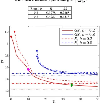
1) Pareto optimal curves: Figure 7 shows the trade-off curve between the imposed upper bound γ1 on Twu
∞ and the obtained upper bound γ2 on
2
wz
T for two bounds b = 0.2 and b = 0.8 on the rate of parameter variation. The bound γ1 takes values in a fine grid of the interval [0;50]. In this figure, the label GS denotes gain-scheduled control designs (solid lines) and the label R denotes robust control designs (dashed lines). For each bound (b = 0.2 and b
= 0.8), one gain-scheduled and one robust H2 controller are calculated without the bound γ1 on Twu
∞ using respectively Theorem 2 and Corollary 2. These four designs (indicated in Fig. 7 with dotted lines for the gain-scheduled case and with dash-dotted lines for the robust case) provide the best achievable upper bound on
2
wz
T , that is, the smallest achievable value for γ2, denoted by γ2. The value of γ2 for each control design case is given in Table 2. As
can be seen from Fig. 7, the mixed H2/H∞control designs always provide a bigger upper bound γ2 > γ2 , thus having worse guaranteed performance compared to the H2 control design. It is also clear that the performance decreases as the bound b on the rate of parameter variation increases. For small values of γ1 the synthesis conditions become infeasible (indicated with squares). As expected, the gain-scheduled controllers GS outperform the robust controllers R.
Table 2. Best achievable upper bound γγγγ2 on
2 wz
T .
Bound b R GS
0.2 0.3278 0.2268
0.8 0.4987 0.4553
Figure 7. Trade-off between the imposed bound γγγγ1 on ∞
wu
T and the
obtained bound γγγγ2 on
2 wz
T .
2) Performance of the gain-scheduled controllers obtained for b
= 0.2: The performance of the gain-scheduled control design for the case b = 0.2 is now analyzed using Bode plots (see Fig. 8) for five equidistantly spaced temperatures in the interval [22.9º; 25.4º]. The following three controllers are compared:
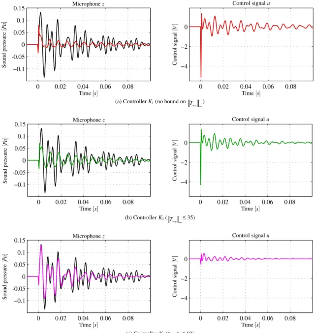
• Controller K1: no upper bound on Twu
∞, yielding the smallest achievable upper bound γ2 on
2
wz
T (Fig. 8a, red);
• Controller K2: upper bound γ1 = 35 on Twu
∞(Fig. 8b, green);
• Controller K3: upper bound γ1 = 10 on Twu
∞(Fig. 8c, magenta).
(a) Controller K1 (no bound on wu
T ∞)
(b) Controller K2 ( wu
T ∞≤ 35)
(c) Controller K3 ( wu
T ∞≤ 10)
Figure 8. Bode magnitude plots of the open-loop system (black) and the closed-loop systems, using controllers K1, K2 and K3 with b = 0.2, for 5
temperatures in the interval [22.9º;25.4º].
From Fig. 8, it is clear that compared to the open-loop system, all controllers improve the H2 performance from the disturbance w to the microphone z, for all temperatures. Controller K1 yields the best H2 performance (see Fig. 8a). However, since no upper bound is imposed on Twu
∞, the red curves in the right side of Fig. 8a have the highest peaks, thus requiring large control authority. Compared to controller K1, controller K2 yields slightly worse H2 performance (as can be seen in the left side of Fig. 8b), but since an upper bound
γ1 = 35 is imposed on Twu ∞, the green curves in the right side of Fig. 8b have slightly smaller peaks compared to those from Fig. 8a.
The third controller K3 is designed with a significantly tighter bound γ1 = 10 on Twu
∞ and consequently the curves in the right side of Fig. 8c are significantly lower compared to the curves associated with K1 and K2.
Thus, controller K3 requires less control authority. However, the obtained H2 performance is also considerably worse, as can be seen in the left side of Fig. 8c.
green diamond) provides a slightly bigger upper bound γ2, but guarantees an upper bound γ1 = 35 on Twu
∞. Controller K3 (indicated with the magenta diamond) provides a significantly bigger upper bound γ2, but guarantees a smaller upper bound γ1 = 10 on
wu
T ∞. The upper bound γ1 = 35 corresponds to 20 log10 35 ≈ 31[dBref=1Pa/N] and is indicated in Fig. 8b with the green dashed line, while the upper bound γ1 = 10 corresponds to 20 log10 10 = 20[dBref=1Pa/N] and is indicated in Fig. 8c with the magenta dashed line.
Figure 9 shows a time domain simulation, where a unit impulse is applied (at t = 0) to the open-loop system and to the closed-loop systems computed using the three controllers K1, K2 and K3 described above. The time interval used for the simulation is t ∈ [0; 0.1]. During the simulation, the scheduling parameter (the temperature) changes randomly in the interval [22.9º; 25.4º] with a bounded rate of variation b = 0.2. The open-loop response from the disturbance w to the microphone z (black) is compared with the closed-loop response computed using the controllers K1 (red), K2 (green) and K3 (magenta). The time simulation empha-sizes again the difference between the 3 controllers. Controller K1 shows the best attenuation of the disturbance (as can be seen in the left side of Fig. 9a), but results in the highest peaks in the control signals (as can be seen in the right side of Fig. 9b). Controller K2 yields slightly worse disturbance attenuation, but has smaller peaks in the control signal (see Fig. 9b).
Finally, controller K3 performs significantly worse in attenuating the disturbance, but does not require large control signals (see Fig. 9c).
Discussion
The numerical results presented in Figs. 7, 8 and 9 show the potential of the proposed multiobjective H2/H∞ gain-scheduled and robust control design techniques. Based on the trade-off curves shown in Fig. 7, a specific controller can be chosen that yields a guaranteed closed-loop H2 performance, while still guaranteeing an upper bound on the H∞ performance from the disturbance w to the control signal u. Certainly, the main drawback of the proposed control design is its current limitation to the state feedback case. In many engineering applications, such as the vibroacoustic setup in this paper, it is impossible to measure all states of the system and consequently full state feedback laws cannot be directly implemented in practice. However, no results yet exist in the literature that provide gain-scheduled dynamic output feedback controllers that consider bounds on the rate of parameter variation. It is important to stress the incorporation of a priori known bounds on the rate of parameter variation into the synthesis procedure, since for the vibroacoustic application, quadratic stability based approaches fail to yield a feasible set of synthesis conditions.
There are two possible strategies that can be used to achieve gain-scheduled dynamic output feedback controllers. The first possibility is to consider the joint design of a gain-scheduled state observer and a gain-scheduled state feedback controller. The second
possibility is to derive synthesis conditions for gain-scheduled dynamic output feedback controllers. These are interesting open questions the authors plan to investigate in future works.
Although no experimental validation is provided in this paper, the proposed state feedback synthesis conditions are valuable for several reasons. First, the state feedback controllers provide the best possible closed-loop performance that can be achieved for the vibroacoustic system. Second, the state feedback synthesis results might be the first step towards the design of a dynamic output feedback controller in the form of a full order observer combined with a state feedback law. Third, the influence of the bound b on the rate of variation can be easily verified by calculating different trade-off curves as presented in Fig. 7. Fourth, this paper also shows that recent theoretical results for LPV control have the potential to be applied to models obtained from experimental data.
Conclusion
This paper shows that recently developed techniques to model and control linear parameter-varying systems can be applied to realistic engineering problems, in this case a vibroacoustic setup whose dynamics are highly sensitive to temperature variation. Based on experimentally obtained FRFs, a set of LTI models is estimated for different fixed temperatures. Then, an LPV model is derived for the vibroacoustic setup by interpolating these local LTI models using the State-space Model Interpolation of Local Estimates (SMILE) technique. Gain-scheduled and robust multiobjective H2/H∞ state feedback controllers are designed using LMI synthesis conditions based on a parameter-dependent Lyapunov matrix. These synthesis procedures consider a priori known bounds on the rate of parameter variation, which reduces the conservatism generally associated with methods that allow arbitrarily fast parameter variation, like the quadratic stability based approaches. Numerical simulations clearly show the advantages and versatility of the proposed modeling and control design procedures.
Acknowledgements
(a) Controller K1 (no bound on wu
T ∞)
(b) Controller K2 ( wu
T ∞≤ 35)
(c) Controller K3 ( wu
T ∞≤ 10)
Figure 9. Impulse response plots of the open-loop system (black) and the closed-loop systems, using controllers K1, K2 and K3 with b = 0.2, subject to a
random variation on the scheduling parameter.
References
Alujevic, N., Frampton, K.D. and Gardonio, P., 2008, “Stability and performance of a smart double panel with decentralized active dampers”,
AIAA Journal, Vol. 46, No. 7, pp. 1747-1756.
Amato, F., Mattei, M. and Pironti, A., 2005, “Gain scheduled control for discrete-time systems depending on bounded rate parameters”, Intern. Journal of Robust and Nonlinear Control, Vol. 15, pp. 473-494.
Aouf, N., Bates, D.G., Postlethwaite, I. and Boulet, B., 2002, “Scheduling schemes for an integrated flight and propulsion control system”,
Control Engineering Practice, Vol. 10, No. 1, pp. 685-696.
Apkarian, P. and Adams, R.J., 1998, “Advanced gain-scheduling techniques for uncertain systems”, IEEE Transactions on Control Systems Technology, Vol. 6, No. 1, pp. 21-32.
Apkarian, P., Gahinet, P. and Becker, G., 1995, “Self-scheduled
H∞control of linear parameter-varying systems – A design example”,
Automatica, Vol. 31, No. 9, pp. 1251-1261.
Bamieh, B. and Giarré, L., 2002, “Identification of linear parameter varying models”, International Journal of Robust and Nonlinear Control, Vol. 12, No. 9, pp. 841-853.
Berglund, B., Hassmén, P. and Job, R.F.S., 1996, “Sources and effects of low-frequency noise”, J. Acoust. Soc. Am., Vol. 99, No. 5, pp. 2985-3002.
Boyd, S., El Ghaoui, L., Feron, E. and Balakrishnan, V., 1994, “Linear Matrix Inequalities in Systems and Control Theory”, Vol. 15 of Stud. Appl. Math. SIAM, Philadelphia.
Camino, J.F. and Arruda, J.R.F., 2009, “H2 and H∞feedforward and
feedback compensators for acoustic isolation”, Mechanical Systems and Signal Processing, Vol. 23, No. 8, pp. 2538-2556.
De Caigny, J., Camino, J.F., Paijmans, B. and Swevers, J., 2007, “An application of interpolating gain-scheduling control”, Proc. of the 3rd IFAC
Symp. Syst., Struct. and Control (SSSC07), Foz do Iguassu, Brazil (cdrom). De Caigny, J., Camino, J.F., Oliveira, R.C.L.F., Peres, P.L.D. and Swevers, J., 2008a, “Gain scheduled H2-control of discrete-time polytopic
De Caigny, J., Camino, J.F., Oliveira, R.C.L.F., Peres, P.L.D. and Swevers, J., 2008b, “Gain-scheduled H∞-control of discrete-time polytopic
time-varying systems”, Proceedings of the 47th IEEE Conference on
Decision and Control, pp. 3872-3877, Cancun, Mexico.
De Caigny, J., Camino, J.F. and Swevers, J., 2008c, “Identification of MIMO LPV models based on interpolation”, Proceedings of the International Conference on Noise and Vibration Engineering, pp. 2631-2644, Leuven, Belgium.
De Caigny, J., Camino, J.F., Oliveira, R.C.L.F., Peres, P.L.D. and Swevers, J., 2009a, “Gain-scheduled H∞-control for discrete-time polytopic
LPV systems using homogeneous polynomially parameter-dependent Lyapunov functions”, Proceedings of the 6th IFAC Symposium on Robust
Control Design, pp. 19-24, Haifa, Israel.
De Caigny, J., Camino, J.F. and Swevers, J., 2009b, “Interpolating model identification for SISO linear parameter-varying systems”,
Mechanical Systems and Signal Processing, Vol. 23, No. 8, pp. 2395-2417. De Caigny, J., Camino, J.F., Oliveira, R.C.L.F., Peres, P.L.D. and Swevers, J., 2010a, “Gain-scheduled H2 and H∞control of discrete-time
polytopic time-varying systems”, IET Control Theory & Applications, Vol. 4, No. 3, pp. 362-380.
De Caigny, J., Camino, J.F. and Swevers, J., 2011, “Interpolation-based modelling of MIMO LPV systems”, IEEE Transactions on Control Systems Technology, Vol. 19, No. 1, pp 46-63.
De Oliveira, M.C., Geromel, J.C. and Bernussou, J., 2002, “Extended H2
and H∞norm characterizations and controller parameterizations for
discrete-time systems”¸ Intern. Journal of Control, Vol. 75, No. 9, pp. 666-679. De Souza, C.E. and Trofino, A. 2006, “Gain-scheduled H2 controller
synthesis for linear parameter varying systems via parameter-dependent Lyapunov functions”, International Journal of Robust and Nonlinear Control, Vol. 16, No. 5, pp. 243-257.
Donadon, L.V., Siviero, D.A., Camino, J.F. and Arruda, J.R.F., 2006, “Comparing a filtered-XLMS and an H2 controller for the attenuation of the
sound radiated by a panel”, Proceedings of the International Conference on Noise and Vibration Engineering, pp. 199-210, Leuven, Belgium.
Felici, F., van Wingerden, J.W. and Verhaegen, M., 2007, “Subspace identification of MIMO LPV systems using a periodic scheduling sequence”,
Automatica, Vol. 43, No. 10, pp. 1684-1697.
Fuller, C.R. and von Flotow, A.H., 1995, “Active control of sound and vibration”, IEEE Control Systems Magazine, Vol. 15, No. 6, pp. 9-19.
Kaiser, O.E., Pietrzko, S.J. and Morari, M. 2003, “Feedback control of sound transmission through a double glazed window”, Journal of Sound and Vibration, Vol. 263, No. 4, pp. 775-795.
Kaminer, I., Khargonekar, P.P. and Rotea, M.A., 1993, “Mixed
H2⊳H∞control for discrete-time systems via convex optimization”,
Automatica, Vol. 29, No. 1, pp. 57-70.
Lee, L.H. and Poolla, K., 1999, “Identification of linear parameter-varying systems using nonlinear programming”, Journal of Dynamic Systems, Measurement, and Control, Vol. 121, No. 1, pp. 71-78.
Leite, V.J.S. and Peres, P.L.D., 2004, “Robust control through piecewise Lyapunov functions for discrete time-varying uncertain systems”,
International Journal of Control, Vol. 77, No. 3, pp. 230-238.
Leith, D.J. and Leithead, W.E., 2000, “Survey of gain-scheduling analysis and design”, Intern. Journal of Control, Vol. 73, No. 11, pp. 1001-1025.
Ljung, L., 1999, “System Identification: Theory for the User”, Prentice-Hall, Upper Saddle River, NJ, USA.
Lovera, M. and Mercere, G., 2007, “Identification for gain-scheduling: a balanced subspace approach”, Proceedings of the American Control Conference, pp. 858-863, New York, NY, USA.
Lu, B., Choi, H., Buckner, G.D. and Tammi, K., 2008, “Linear parameter-varying techniques for control of a magnetic bearing system”,
Control Engineering Practice, Vol. 16, No. 10, pp. 1161-1172.
Meurers, T., Veres, S.M. and Elliot, S.J., 2002, “Frequency selective feedback for active noise control”, IEEE Control Systems Magazine, Vol. 22, No. 4.
Montagner, V.F., Oliveira, R.C.L.F., Peres, P.L.D. and Bliman, P.-A., 2007, “Linear matrix inequality characterization for H∞and H2 guaranteed
cost gain-scheduling quadratic stabilisation of linear time-varying polytopic systems”, IET Control Theory & Applications, Vol. 1, No. 6, pp. 1726-1735.
Moore, B.C., 1981, “Principal component analysis in linear systems: Controllability, observability, and model reduction”, IEEE Transactions on Automatic Control, Vol. 26, No. 1, pp. 17-32.
Nemani, M., Ravikanth, R. and Bamieh, B.A., 1995, “Identification of linear parametrically varying systems”, Proceedings of the 34th IEEE
Conference on Decision and Control, pp. 2990-2995, New Orleans, LA, USA. Nichols, R.A., Reichert, R.T. and Rugh, W.J., 1993, “Gain scheduling for H-infinity controllers: A flight control example”, IEEE Transactions on Control Systems Technology, Vol. 1, No. 2, pp. 69-79.
Oliveira, R.C.L.F. and Peres, P.L.D., 2008, “Robust stability analysis and control design for time-varying discrete-time polytopic systems with bounded parameter variation”, Proceedings of the American Control Conference, pp. 3094-3099, Seattle, WA, USA.
Packard., A., 1994, “Gain scheduling via linear fractional transformations”, Systems & Control Letters, Vol. 22, No. 2, pp. 79-92.
Paijmans, B., Symens, W., van Brussel, H. and Swevers, J., 2008, “Experimental identification of affine LPV models for mechatronic systems with one varying parameter”, European Journal of Control, Vol. 14, No. 1, pp. 16-29.
Peres, P.L.D., Geromel, J.C. and Souza, S.R., 1994, “H2 output feedback
control for discrete-time systems”, Proceedings of the American Control Conference, pp. 2429-2433, Baltimore, MD, USA.
Persson, K. and Björkman, M., 1988, “Annoyance due to low frequency noise and the use of the dBA scale”, Journal of Sound and Vibration, Vol. 127, No. 3, pp. 491-497.
Rugh, W.J. and Shamma, J.S., 2000, “Research on gain scheduling”,
Automatica, Vol. 36, No. 10, pp. 1401-1425.
Sas, P., Bao, C., Augusztinovicz, F. and Desmet, W., 1995, “Active control of sound transmission through a double panel partition”, Journal of Sound and Vibration, Vol. 180, No. 4, pp. 609-625.
Scherer, C.W., 2001, “LPV control and full block multipliers”,
Automatica, Vol. 37, No. 3, pp. 361-375.
Shamma, J.S. and Athans, M., 1991, “Guaranteed properties of gain scheduled control for linear parameter-varying plants”, Automatica, Vol. 27, No. 3, pp. 559-564.
Shamma, J.S. and Athans, M., 1992, “Gain scheduling: potential hazards and possible remedies”, IEEE Control Systems Magazine, Vol. 12, No. 3, pp. 101-107.
Steinbuch, M., van de Molengraft, R. and van der Voort, A., 2003, “Experimental modelling and LPV control of a motion system”, Proceedings of the American Control Conference, pp. 1374-1379, Denver, CO, USA.
Van Overschee, P. and Moor, B.L., 1996, “Subspace Identification for Linear Systems: Theory - Implementation - Applications”, Kluwer Academic Publishers, Norwell.
Verdult, V. and Verhaegen, M., 2005, “Kernel methods for subspace identification of multivariable LPV and bilinear systems”, Automatica, Vol. 41, No. 9, pp. 1557-1565.
Verhaegen, M., 1994, “Identification of the deterministic part of MIMO state-space models given in innovations form from input-output data”,
Automatica, Vol. 30, No. 1, pp. 61-74.
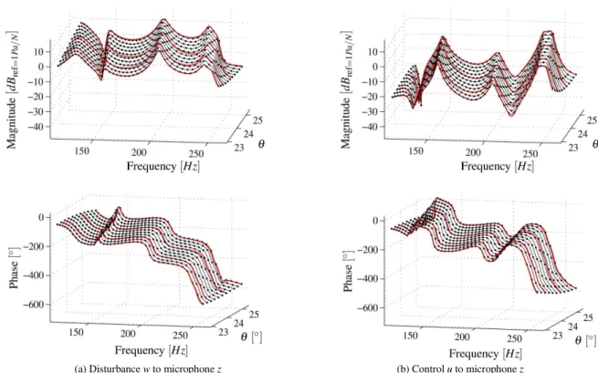
![Figure 5 compares the 4 local LTI MIMO models (red, solid) to the obtained interpolating LPV model (black, solid with dots), evaluated at 11 equidistantly spaced temperatures in the interval [22.9º; 25.4º]](https://thumb-eu.123doks.com/thumbv2/123dok_br/18975629.455236/4.892.476.763.818.890/figure-compares-obtained-interpolating-evaluated-equidistantly-temperatures-interval.webp)
![Figure 8. Bode magnitude plots of the open-loop system (black) and the closed-loop systems, using controllers K 1 , K 2 and K 3 with b = 0.2, for 5 temperatures in the interval [22.9º;25.4º]](https://thumb-eu.123doks.com/thumbv2/123dok_br/18975629.455236/8.892.98.792.130.892/figure-bode-magnitude-closed-systems-controllers-temperatures-interval.webp)