Robustness of Spontaneous Pattern Formation in Spatially
Distributed Genetic Populations
M.A.M. de Aguiar
1,2, M. Baranger
2,3, Y. Bar-Yam
2,4, and H. Sayama
5 1Instituto de F´ısica Gleb Wataghin, Universidade Estadual de Campinas, 13083-970 Campinas, S ˜ao Paulo, SP, Brazil
2
New England Complex Systems Institute, Cambridge, Massachusetts 02138, USA
3
Physics Department, University of Arizona, Tucson, Arizona 85721, USA
4
Department of Molecular and Cellular Biology, Harvard University, Cambridge, MA 02138, USA
5
Department of Human Communication, University of Electro-Communications, Chofu, Tokyo 182-8585, Japan
Received on 16 April, 2003
Spatially distributed genetic populations that compete locally for resources and mate only with sufficiently close neighbors, may give rise to spontaneous pattern formation. Depending on the population parameters, like death rate per generation and size of the competition and mating neighborhoods, isolated groups of individuals, or demes, may appear. The existence of such groups in a population has consequences for genetic diversity and for speciation. In this paper we discuss the robustness of demes formation with respect to two important characteristics of the population: the way individuals recognize the demarcation of the local neighborhoods and the way competition for resources affects the birth rate in an overcrowed situation. Our results indicate that demes are expected to form only for sufficiently sharp demarcations and for sufficiently intense competition.
I
Introduction
Animals don’t live completely free in the wild because their living space is confined by natural boundaries. The size of the area used is determined often by individual and species needs and environmental limitation. Within the geographic distribution of the species, therange, only areas of suitable habitat are occupied.
The living area normally inhabited by an animal is its
Home Range. It may belong to a single individual, a mated pair, or a social unit. Within the home range there is of-ten a defended area which is identified as aterritory. Typi-cal behavior is usually associated with establishing and de-fending or protecting the animal’s territory. This behavior and the reproductive behavior associated with the territory is unique for each species, and allows several different ani-mal species to live in the same space without rivalry, using different niches within the habitat. Territories are marked so that other members of the species can recognize it. Opti-cal, acoustic, or olfactory cues, or a combination of these are often used. Olfactory demarcation is very common among mammals with a well-developed sense of smell. Urine, fe-ces and products of special scent glands are used alone or in conjunction to mark out the territory.
Theoretical biologists have become increasingly aware of the importance of space in ecology, evolution and epi-demiology. Home ranges and territories have become im-portant parameters in mathematical models of population dynamics [1, 2]. It has also become apparent that inho-mogeneities in spatially distributed populations can funda-mentally change the dynamics of these systems [3-10]. The
spatial variations so common to species in the wild, for in-stance, is usually attributed to variations in selective forces, i.e., differences in the environment. However, it has been shown that spatially distributed systems can develop in-homogeneity through symmetry breaking and spontaneous pattern formation, independently of environmental inhomo-geneity [11, 12]. Understanding the mechanisms that may lead to spatial inhomogeneities, and the eventual isolation of groups, is of fundamental importance for the study of ge-netic diversity and speciation [14-18].
In a previous paper [12] we studied the process of pattern formation in spatially distributed evolutionary processes us-ing a model involvus-ing population density variations and ge-netic variations. The main ingredient of the model is the assumption that individuals mate and compete for resources only locally. The competing neighborhood can be associ-ated with the territory. The mating neighborhood is a dif-ferent range, where the individual looks for a mate. The size of these neighborhoods play a crucial role in the spa-tial equilibrium configuration attained by the system. In this paper we show that, in fact, it is not only the size of these neighborhoods that matters, and we explore the way neigh-borhoods are identified by the individuals as a key element in the formation of isolated groups.
we consider three different types of what we callcrowding functionsand study their influence in the process of pattern formation. We are interested in studying the robustness of these patters with respect to variations in the crowding func-tions and the sharpness of the boundaries. What we mean by robustness with respect to a parameter or function is that the patterns continue to appear if the parameter or function is modified slightly.
Our main conclusion is that isolated groups, or demes, form only if competition for resources is sufficiently intense, in the sense that lack of resources implies a drastic reduction of the birth rate, and if territories are marked sufficiently sharply. If territory boundaries are too fuzzy, the overlap be-tween demes leads to a single homogeneous group. In order to focus on the population density, we shall simplify the ge-netic variations enormously, taking only four interbreeding genomes with equally fit genotypes.
The paper is organized as follows: in section II we de-scribe our model, in section III we discuss the spatially ho-mogeneous solutions, and in section IV we study their sta-bility as function of the several parameters describing the population behavior. Demes arise when these homogeneous solutions become unstable. We check our analytical findings with numerical simulations of the spatial model. In section V we summarize our conclusions.
II
Model
We consider a population distributed over a large two-dimensional region. For the sake of computational conve-nience, space will be considered discrete, and the popula-tion located in a square lattice with periodic boundary con-ditions. We use the notation~r or~rij = (xi, yj)for a point on the 2-D lattice. The local population densities on each
site of the grid consists of non-negative real numbers with no predefined upper bound.
For most living organisms the genome contains thou-sands of genes. Here we shall focus on only two genes, each of which is assumed to have only two alleles. The indi-viduals reproduce sexually, so that one copy of each gene is inherited from each of the parents. Representing the alleles by the symbols+and−, we have four possible genotypes:
[+,+],[+,−],[−,+]and[−,−]. The genotypes can repre-sent either a two-locus haploid genetics where gene recom-bination is enforced in every mating, or one-locus diploid genetics if[+,−]and[−,+]are identified with each other. For simplicity we assume that any pair of individuals can mate to produce offspring, i.e., we make no distinction be-tween males and females. We use the notationnαβ(~r)or
nt
αβ(~r)to denote the population of genotype[α, β]at site~r and time t.n(~r)ornt(~r)is used for the total population.
The population at each site is updated at discrete time intervals. At each time step (breeding season), offspring are born and part of the previous population dies. Sexual reproduction between individuals introduces genetic mix-ing. We assume that individuals mate preferentially with nearby members of the population, i.e., mating takes place within localmating neighborhoodsthat range over several sites. Genetic mixing, therefore, occurs only locally. The total number of offspring born per site per breeding season is bounded by the introduction of an intrinsic carrying ca-pacity, modeling a limitation of resources for reproduction.
Finally, competition for finite resources also takes place locally, within competition neighborhoods, ranging again over several sites, but whose size may be different from that of the mating neighborhoods.
The general form of the iterative equation for the local population on each site is
⌋
n′
αβ(r) = σαβnαβ(r) +λαβhn(r)iM h
nα∗(r)iM
hn(r)iM
hn∗β(r)iM
hn(r)iM
f(hn(r)iC)
= σαβnαβ(r) +λαβhnα∗(r)iMhn
∗β(r)iM
hn(r)iM
f(hn(r)iC) (1)
⌈
whereσαβis the survival rate of the parents,λαβis the re-productive rate, M is the mating neighborhood, C is the competition neighborhood, nα∗ = nα+ +nα−, n∗β =
n+β+n−β. The prime on the left-hand-side indicates the population at timet+ 1and the angular brackets denote av-erage over the indicated neighborhood. The functionf on the right-hand-side is the crowding function. Its role is to limit the average population over the competition neighbor-hood C. We shall discuss the crowding function and the neighborhood types shortly. The genetic composition of the newborns is determined by the product of two allelic proba-bilities averaged within the mating neighborhood.
of the population being considered. Here we shall only con-sider simple functions to model competition, but that will be enough to highlight the importance of f in the process of pattern formation. To simplify the notation we shall mea-sure populations in units of the site capacity, which amounts to makeK= 1in all equations.
The average value hxi can be defined in a number of ways. In our original work [12] this average was computed using the so called characteristic function of the neighbor-hood, which is 1 for points inside a certain radius around the site and0for points outside. However, sharp boundaries are not likely to occur in practice, and the definition of ter-ritorial boundaries might vary from organism to organism. We have shown, in particular, that Gaussian averages never lead to the formation of demes for a logistic type of crowd-ing function. We shall show in this paper that the sharpness of boundaries turns out to be a crucial parameter for pattern formation.
As a last remark we emphasize the role of the model pa-rameters to the issue of territoriality. The size and shape of the competition neighborhoodCdefines the individual’s ter-ritory. The mating neighborhoodM defines the area around the home range where the individual looks for a mate (in the case of birds this is also termed thebreeding dispersal
range, and it usually larger than the territory [18]). We shall describe neighborhoods by a two-parameter family of func-tions, containing information about the size of the rangeand
sharpness of the range boundaries. We shall focus on the neighborhood sharpness, keeping the sizes fixed. Finally, the crowding function controls theeffectivenessof competi-tion, i.e., how the birth rate decreases when the population grows close to the site capacity. As examples, we shall con-sider three types of crowding functions.
II.1 The Flat Fitness Case
Our main goal here is to investigate the role of compe-tition in the process of demes formation. In order to fo-cus on this issue we shall restrict ourselves to theflat fitness
case, where all types have identical death and birth rates. In this case the only relevant parameter is the total population
n=n+++n−−+n+−+n−+and the dynamical equation fornsimplifies to
n′
(~r) =σn(~r) +λhn(~r)iRMf(hn(~r)iRC). (2)
II.2 The Crowding Function
In our model, competition acts through two separate mechanisms: the crowding functionf, which controls how the birth rate decreases when the population increases be-yond the average site capacity, and the competition neigh-borhood itself. The crowding function has to satisfyf(0) = 1andf(x)<1forx >0. We shall consider three types of
functions here:
f(x) =
½
1−x if x <1
0 if x >1 ( Logistic)
f(x) =e−x (Exponential)
f(x) =e−x2
(Gaussian)
(3)
II.3 Neighborhoods
The average of n(~r) depends on the definition of the neighborhoods. Since space is homogeneous and isotropic, we restrict ourselves to circular neighborhoods. We write
hn(~r)iR=
Z ∞
0
n(~r′
)ρR(r−r′)2πr′dr′ (4) with
2π
Z ∞
0
ρR(r)rdr= 1. (5)
ρis the averaging, or smoothing, function. It tells how sharply the territorial boundaries are identified by the in-dividuals. Sharp boundaries correspond to taking ρas the characteristic function of the neighborhoodR:
ρR(r) =
1
πR2
1 if r≤R
0 if r > R .
(6)
In order to generalize the way the averages are per-formed, and therefore the way territories are marked, we define the two-parameter family of smoothing functions
ρR,α(r) =N
1
1 +e(r−R)/α (7) with normalization
N−1= 2πZ
∞
0
rdr
1 +e(r−R)/α =−2πα
2P olyLog[2,
−eα/R]
(8) where
P olyLog[2, z] = ∞
X
k=1
zk
2k . (9)
αis the smoothing parameter. It is zero for the sharp av-erage, Eq.(6). As αgrows from zero the neighborhood’s boundary becomes more and more diffuse.
III
Homogeneous Solutions
Homogeneous (space independent) solutions satisfy the dy-namical equation
n′
=σn+λnf(n). (10) There are two stationary solutions, wheren′
=n:
n0= 0 (extinction) (11)
and
f(n0) =
1−σ
The stability of these homogeneous stationary solutions are determined by the behavior of small perturbations. For extinction we writen= 0 +δnand obtain, to first order in
δn,
δn′
=σδn+λδnf(0)
= (σ+λ)δn . (13)
Therefore extinction is stable ifσ+λ < 1and unstable if
σ+λ >1.
For the second solution we first note that the equation forn0can be writtenf(n0) = 1 + (1−σ−λ)/λ. Since we assumef(n0)<1forn0>0, we must have1−σ−λ <0. Therefore thriving is possible only ifσ+λ >1. Expanding Eq.(10) aroundn0we obtain
δn′ =
µ
1 +λn0
∂f ∂n(n0)
δn . (14)
Since∂f /∂n <0, the thriving solution starts stable asσ+λ
grows from1. The stability range, however, depends of the particular crowding function one uses. For the three func-tions listed in Eq.(3) we get the following explicit solufunc-tions and stability conditions:
(a) Logistic
n0= (σ+λ−1)/λ , (15) stable if1< σ+λ <3.
(b) Exponential
n0= log [λ/(1−σ)], (16) stable if0<(1−σ) log [λ/(1−σ)]<2.
(c) Gaussian
n0=
p
log [λ/(1−σ)], (17) stable if0<(1−σ) log [λ/(1−σ)]<1.
IV
The Dynamics of Demes
Forma-tion
Spatial patterns arise when the homogeneous solutions be-come unstable under smallspatialperturbations. Let us look for solutions of eq.(2) in the linear approximation, assuming them to be of the form
n(~r) =n0+ξ µts(~r) (18) where
s(~r) = sin (vx+φ) sin (wy+ψ) (19) represents a spatial perturbation of specific wavelength,µt is an exponential time-dependence, possibly complex, andξ
is a small coefficient. We shall insert (18) into (2) and study the change ofµtover one time-step, to find out under what circumstancesn0becomes unstable. To do that we need to
calculate the average of the perturbation over the mating and competing territories,hs(~r)iR. We find
hs(~r)iR=s(~r)AR,α(k) (20) where
AR,α(k) = 2π
Z ∞
0
rJ0(kr)ρR,α(r)dr , (21)
with k = √v2+w2. The effect of the averaging is to
renormalizethe amplitude of the perturbation. We shall call
AR,α(k)theAmplitude Factorand we note that it depends on the wavelength of the perturbation.
Inserting Eq.(7) into Eq.(21) we find
AR,α(k) =−
1
ω2
I(r, ω)
P olyLog(2,−er/ω) (22) where
I(r, ω) =
Z ∞
0
uJ0(u)
1 +e(u−r)/ωdu , (23)
r=Rk,J0is the Bessel function of order zero andω=αk. Finally, inserting (18) into (2) and expanding to first or-der inξwe obtain an equation forµafter one time-step:
µ=σ+(1−σ)ARM,α(k)+λ n0
∂f
∂n(n0)ARC,α(k). (24) The homogeneous solutionn0is unstable under spatial perturbations ifµ > 1. For the three crowding functions listed in section II we obtain the following conditions for instability:
(a) Logistic
σ+ (1−σ)ARM,α−(λ+σ−1)ARC,α>1 (25) or
h≡1−ARM,α+
λ+σ−1
1−σ ARC,α< 0. (26) (b) Exponential
σ+(1−σ)ARM,α−(1−σ) log
µ
λ
1−σ
ARC,α>1 (27) or
h≡1−ARM,α+ log
µ λ
1−σ
ARC,α < 0. (28) (c) Gaussian
σ+ (1−σ)ARM,α−2(1−σ) log
µ
λ
1−σ
ARC,α>1 (29) or
h≡1−ARM,α+ 2 log
µ λ
1−σ
ARC,α < 0. (30) In the limit of a sharply defined neighborhood,α→ 0
(orω→0) we get
I(r,0) =
Z r
0
lim
ω→0[P olyLog(2,−e r/ω)] =
−12[log (1 +er/ω)]2=− r
2
2ω2 (32) and
AR,0(k) = 2J1(r)
r . (33)
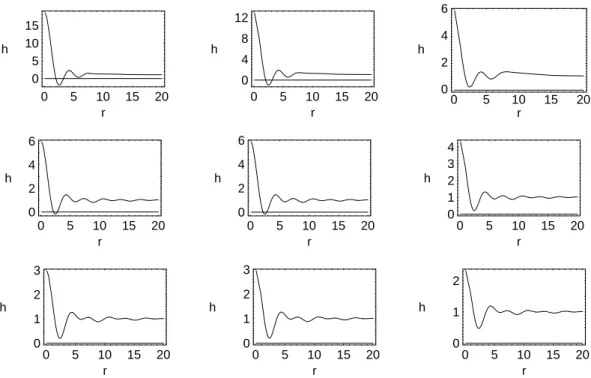
Figure 1 shows plots of has a function of r = Rmk for different values of ω = αk. In all cases RM = 5,
RC = 10, λ = 2.0 and σ = 0.9. The regions where
h <0indicate instabilities of the homogeneous distribution. The value ofrwhere the negative minimum occurs,r0, con-tains information about the size of the spatial structures that should form as a result of the perturbation. For fixedRM we findk0≡r0/RM andλ0≡2π/k0as the critical pertur-bation wavelength under which the homogeneous solutions become unstable. This is the approximate size of the demes that are formed. From the figures we findr0 ≈2.5, which givesλ0≈15.
0 5 10 15 20
r 0
5 10 15
h
0 5 10 15 20
r 0
4 8 12
h
0 5 10 15 20
r 0
2 4 6
h
0 5 10 15 20
r 0
2 4 6
h
0 5 10 15 20
r 0
2 4 6
h
0 5 10 15 20
r 0
1 2 3 4
h
0 5 10 15 20
r 0
1 2 3
h
0 5 10 15 20
r 0
1 2 3
h
0 5 10 15 20
r 0
1 2
h
Figure 1. Stability functionh(r)for the three crowding functions. Top: logistic function forω = 0.1,0.5and1.0; Middle: Gaussian function forω= 0.05,0.1and0.5; Bottom: exponential function forω= 0.05,0.1and0.5. In all casesRM = 5,RC= 10,λ= 2.0and σ= 0.9.
For the logistic type of competition function (first three plots), the homogeneous solution is stable against perturba-tions of any wavelength ifω &0.8. Fixingk0=r0/Rm=
0.5we find a critical smoothing parameterα0 = ω/k0 ≈
1.6. For the Gaussian competition function the homoge-neous solution is stable ifω&0.25, which givesα0≈0.5. Finally, for the exponential function the homogeneous solu-tion is expected to be always stable, completely preventing the appearance of demes.
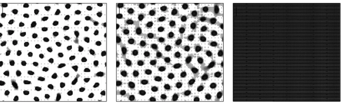
In order to confirm these predictions we show in Figs. 2 and 3 the results of numerical simulations with our spa-tial model. We have used a grid of 128 by 128 points with periodic boundary conditions. The initial configuration for the time evolution is the uniform homogeneous solution plus a small random spatial perturbation. All simulations with the exponential crowding function resulted indeed in spa-tially homogeneous populations and we do not show them here. Fig. 2 corresponds to the logistic crowding function and Fig. 3 to the Gaussian crowding function. In both cases
demes form forαsufficiently small, according to our analyt-ical predictions. The simulations also show that the logistic type of competition leads to faster deme formation than the Gaussian type.
V
Conclusion
The main reason for the existence of territories is competi-tion for finite resources. In the case of animals, competicompeti-tion is usually for food; in the case of plants it may be light. For substrate organisms it may be space [19]. In our pre-vious paper we showed that spatially isolated groups may form spontaneously for populations that mate and compete for resources locally, assuming a logistic type of crowding function and sharp demarcation of territories.
Figure 2. Spatial distribution of the population for the case of a logistic crowding function. From left to rightα= 0.5,1.0and2.0. Demes are seen in the first two cases, but not the third. The dynamical equations were integrated for T=128 time steps. Space consists of a discrete grid with 128 by 128 points and periodic boundary conditions. The population parameters are the same as in Fig.1.
Figure 3. Spatial distribution of the population for the case of a Gaussian crowding function. From left to rightα= 0.1,0.5and1.0. Demes are seen in the first two cases, but not the third. The dynamical equations were integrated forT = 512forα= 0.1and forT = 1024for α= 0.5and1.0. Space consists of a discrete grid with 128 by 128 points and periodic boundary conditions. The population parameters are the same as in Fig.1.
as seen by individuals. We have shown that both of these factors can be decisive in defining the population density profile over the species range. If competition is sufficiently intense, the population divides spontaneously into isolated groups. The territory (deme) boundaries are dictated by (av-erage) individual characteristics, such as death and birth rate per generation, and group factors, such as the size, shape and sharpness of local mating and competition neighborhoods. Among the crowding functions considered, the logistic leads to faster formation of demes and is the most robust against changes in the smoothness of the boundaries. But even a logistic type of crowding cannot garantee the formation of demes if the demarcation of territories is too fuzzy.
Once isolated demes are established, genetic mixing between demes is largely reduced, although some mixing might still occur via inter-demes migration [13, 14, 9]. As we have shown in [12], this spatial isolation contributes to the maintenance of genetic diversity in the presence of disruptive selection. In this case, when, for instance, het-erozigous individuals[+,−]are less fit than homozigous in-dividuals,[+,+]or[−,−], homogeneous populations tend
to be either all[+,+]or all[−,−]. When demes form, the population in each deme is still either all[+,+]or all[−,−], but different demes may be inhabited by different types. In the long run, genetic isolation might also lead to genetic divergence, since random mutations are not shared among demes.
References
[1] V. C. Wynne-Edwards,Animal Dispersion in Relation to So-cial Behavior(Hafner, New York, 1962).
[2] V. C. Wynne-Edwards, Nature200, 623 (1963).
[3] D. Tilman, and P. Kareiva, Spatial Ecology: The Role of Space in Population Dynamics and Interspecific Interactions (Princeton Univ. Press, Princeton, NJ, 1997).
[4] S. A. Levin and L. A. Segel, SIAM Rev.27, 45 (1985). [5] R. Durrett and S. A. Levin, Philos. Trans. R. Soc. London,
Ser. B343, 329 (1994).
[7] E. M. Rauch, H. Sayama, and Y. Bar-Yam, Phys. Rev. Lett.
88, 228101 (2002)
[8] E. M. Rauch, H. Sayama, and Y. Bar-Yam, J. Theor. Biol.
221, 655 (2003).
[9] M.A.M. de Aguiar, H. Sayama, E. Rauch, M. Baranger, and Y. Bar-Yam, Phys. Rev. E65, 31909 (2002).
[10] J. E. Satulovsky and T. Tome, Phys. Rev. E49, 5073 (1994). [11] H. Sayama, L. Kaufman, and Y. Bar-Yam, Phys. Rev. E62,
7065 (2000).
[12] H. Sayama, M.A.M. de Aguiar, Y. Bar-Yam, and M. Baranger, Phys. Rev. E65, 051919 (2002).
[13] S. Wright, Genetics16, 97 (1931). [14] S. Wright, Am. Nat.131, 115 (1988).
[15] J. F. Crow, W. R. Engels, and C. Denniston, Evolution 44, 233 (1990).
[16] S. Gavrilets, Evolution50, 1034 (1996). [17] P. C. Phillips, Evolution50, 1334 (1996).
[18] J. Belliure, G. Sorci, A. P. Moeller, and J. Clobert, J. Evol. Biol.13, 480 (2000).