Influence of the Solar and Density Perturbations
on the Neutrino Parameters
N. Reggiani,
Centro de Ciˆencias Exatas, Ambientais e de Tecnologias, Pontif´ıcia Universidade Cat´olica de Campinas, Caixa Postal 317, 13020-970 Campinas, SP, Brasil
M. M. Guzzo, and P. C. de Holanda
Instituto de F´ısica Gleb Wataghin, Universidade Estadual de Campinas - UNICAMP, 13083-970, Campinas, S˜ao Paulo, Brasil
Received on 2 February, 2004
There are reasons to believe that the solar matter density fluctuates around an equilibrium profile. One of these reasons is a resonance between the Alfv´en waves and the g-modes inside the Sun that creates spikes in the density profile. The neutrinos are created in the solar core and passing through these spikes feel them as a noisy perturbation, whose correlation length is given by the distance between the spikes. When we consider these perturbations on the density profile, the values of the neutrino parameters necessary to obtain a solution to the solar neutrino problem are affected. In particular, in the present work, we show that the values of the parameters of mass and mixing angle that satisfy both the Large Mixing Angle solution to the solar neutrinos and the data from KamLAND - that observes neutrinos created in earth nuclear reactors - are shifted in the direction of lower values as the amplitude of the density noise increases. This means that, depending on the new data of KamLAND and other detectors, it can be necessary to invoke random perturbations in the Sun to recover compatibility with solar neutrino observations. In this case, the neutrino observations will be used as a real probe of the solar interior, giving information of the density profile in the central part of the Sun, which can not be observed directly.
1
Introduction
After the release of KamLAND data [1], it is accepted that the solution to the solar neutrino problem involves the Large Mixing Angle (LMA) realization of the MSW me-chanism [2, 3]. This experiment detected a suppression of a anti-neutrinoν¯e flux that were created in several nuclear
reactors placed at different distances from the Kamiokande site. Interpreting this suppression as oscillation between the ν¯e and anti-neutrino of another flavor, the analysis of
KamLAND data leads to a region for the neutrino para-meters fully compatible with the LMA one [4]. Besides, KamLAND result discards all other neutrino parameter re-gions based on mass induced oscillations [5], such as other possible mechanism for solving the solar neutrino discre-pancy, including non-standard neutrino interactions [6-8], resonant spin-flavor precession (RSFP) in solar magnetic fi-eld [9-12] and violation of the equivalence principle [13-16]. The best fit values of the relevant neutrino parameters that explains both the solar neutrino and KamLAND data are
∆m2 = 7.1×10⁻⁵eV2andsin22θ = 0.39with a boron
neutrino flux normalization offB = 1.04[4].
Besides, when we consider also the solution to the at-mospheric neutrino anomaly in terms of mass induced os-cillations [17] between the second and third neutrino fami-lies, and the limits in the mixing angle θ13 given by the CHOOZ experiment [18], we conclude that the oscillations
of solar neutrinos is in fact induced only by one mass scale
∆m2
21=m22−m21.
But although all the mentioned mechanisms can not be the main one responsible for the solar neutrino deficit, it is interesting to explore if they can play a role as a sub-dominant effect in solar neutrino flavor conversion [19, 20]. Recent analysis also indicated that the solar neutrino flux detected by Super-Kamiokande is variable [21], fact that can not be easily accommodated in the pure LMA solution. Although there are some discussions if this variability is real or just a statistical fluctuation [22, 23], it is interesting to keep in mind that such variability could indicate other me-chanism besides the LMA acting on neutrino conversions in Sun.
2
Random density perturbations in
solar matter
There are reasons to believe that the solar matter density fluctuates around an equilibrium profile. Indeed, in the hydro-dynamical approximation, density perturbations can be induced by temperature fluctuations due to convection of matter between layers with different temperatures. Con-sidering a Boltzmann distribution for the matter density, these density fluctuations are found to be around 5% [24]. Another estimation of the level of density perturbations in the solar interior can be given considering the continuity equation up to first order in density and velocity perturba-tions and the p-modes observaperturba-tions. This analysis leads to a value of density fluctuation around 0.3% [25]. The mecha-nism that might produce such density fluctuations can also be associated with modes excited by turbulent stress in the convective zone [26].
Considering helioseismology, there are constraints on the density fluctuations which would make it very unlikely that such fluctuations could lead to observational effects in solar neutrinos [27]. For the p-waves, the observed wave amplitude is too small in the solar radiative zone to affect neutrino evolution. And for the g-waves, which can have a sizeable amplitude in the solar radiative zone, the wave-length is much larger than the neutrino oscillation wave-length, and again no effect in neutrino propagation is expected.
But recently a new mechanism [28, 29] has been pro-posed to generate density fluctuations with a large enough amplitude and a short enough wavelength to affect the so-lar neutrino oscillation. In this mechanism the shape of the g-waves can be significantly modified by a level crossing between Alfv´en waves associated with a magnetic field in solar radiative zone and the g-modes. As the g-modes occur within the solar radiative zone, these resonance creates spi-kes at specific radii within the Sun. It is not expected that these resonances alter the helioseismic analyses because as they occur deep inside the Sun, they do not affect substanti-ally the observed p-modes.
Before KamLAND results, it has been argued [30] that if a variability would be detected in solar neutrino flux, this could only be generated by fluctuations in solar magnetic field with the same frequency, indicating that the RSFP me-chanism were acting in the solar neutrino evolution. Since the LMA region has now been established as the solution to the solar neutrino problem, discarding the RSFP mechanism as the responsible for neutrino conversion, the claimed link between solar magnetic field oscillations and solar neutrino flux variability should take a more indirect way, as for ins-tance, the resonance between g-modes and Aflv´en waves.
This resonance depends on the density profile and on the solar magnetic field, and as mentioned in Ref. [29], for a magnetic field of order of 10 kG the spacing between the spikes is around 100 km. The resulting wave form depends on details of the magnetic field in the solar radiative zone. For instance, if we have a vanishing radial magnetic field (Br= 0in polar coordinates), but with non-zero theta
com-ponentBθ, the resonance would arise in all directions from
the Sun center. This may trap the g-waves inside the reso-nance and, although having a strong effect in neutrino
evolu-tion, can make them even more difficult to observe. If such field has a dipole form, the conditions needed to the presence of such spikes can only be realized in solar equator. As a re-sult, only solar neutrinos detected in Earth in some periods of the year (December and June), when such neutrinos cross the solar equator, would feel those density fluctuations, and a possible seasonal variation of electron neutrino detection could arise [29].
In this paper we consider the case in which the solar mat-ter density fluctuates by a random noise added to an ave-rage value. This is a reasonable case, considering that in the lower frequency part of the Fourier spectrum, the p-modes resembles that of noise [24]. Also, considering the reso-nance of g-modes with Alfv´en waves, the superposition of several different modes results in a series of relatively sharp spikes in the radial density profile. The neutrino passing th-rough these spikes feel them as a noisy perturbation whose correlation length is the spacing between the density spi-kes [28].
3
Neutrino Evolution
As stated in section 1, we will consider that conversions in-volves only one mass scale, and can be well described by the following 2x2 hamiltonian:
i ddr
µ
νe
νy
=
µ
He Hey
Hey Hy
¶ µ
νe
νy
, (1)
where
He= 2[Aey(t) +δAey], (2)
Hy= 0, Hey≈
∆m2
4E sin 2θ, (3) Aey(t) =
1 2
·
Vey(t)−
∆m2
4E cos 2θ
¸
, (4)
δAey(t)≈
1
2Vey(t)ξ. (5)
HereEis the neutrino energy,θis the neutrino mixing angle in vacuum,∆m2is the neutrino squared mass diffe-rence and the matter potential for active-active neutrino con-version reads
Vey(t) =
√
2GF
mp
ρ(t)(1−Yn), (6)
whereVeyis the potential,GFis the Fermi constant,ρis the
matter density,mpis the nucleon mass andYnis the neutron
number per nucleon. ξis the fractional perturbation of the matter potential.
To calculate the effect of the random perturbation in mat-ter potential, we follow the method presented in [31], where the evolution equation can be rewritten as the following:
˙
P(t) = 2HeyI(t)
˙
R(t) = −HeyI(t)
˙
where P(t) = |νe|2, R(t) = Re(νy∗νe) and I(t) =
Im(ν∗
yνe).
Assuming that after a typical distance L(t), called the correlation length of the perturbation, the density fluctuati-ons are completely spatially uncorrelated, we can average equations (7) over one correlation length. The randomness of density fluctuations are implemented assuming that:
< δAey(t)>=
Rt+L(t)
t Aey(t)dt
L(t) = 0 , (8)
and
< δA2ey(t)>= 1
4Vey(t)< ξ
2(t)> . (9) Generalizing the above relations to higher order, we have:
< δA2eyn+1> = 0,
< δAey(t)δAey(t1)> = 2k(t)δ(t−t1), (10) where the quantityk(t)is defined by
k(t) =< δA2
ey(t)> L(t) =
1 2V
2
ey(t)< ξ2> L(t). (11)
Using these relations, and after some calculations, we can write the averaged products:
< δAey(t)R(t)> = −k(t)< I(t)>
< δAey(t)I(t)> = k(t)< I(t)> ,
(12) and replacing in eq. (7), we can write:
<P˙(t)> = 2Hey< I(t)>
<R˙(t)> = −2Aey(t)< I(t)>−k(t)< R(t)>
<I˙(t)> = 2Aey(t)< R(t)>−2k(t)< I(t)>
−Hey(2< P(t)>−1). (13)
This approximation holds if the characteristic neutrino matter oscillation length is much bigger than the correlation length, soL(t)must obey the following relations:
lf ree<< L(t)<< λm(t), (14)
wherelf reeis the mean free path of the electrons in the Sun
and λm(t) is the characteristic neutrino matter oscillation
length.
In order to guarantee that this condition is satisfied in the whole trajectory of the neutrino inside the sun, we assume that
L(t) = 0.1λm(t) = 0.1
2π
ω(t), (15)
whereω(t)is the frequency of the MSW effect, given by
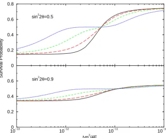
ω2(t) = 4(A2ey(t) +Hey2 ). (16) We use eq. (13) to solve the neutrino evolution, and to calculate its survival probability. In Fig. 1 we show the sur-vival probability for 4 values of the parameterξ,0,2%,4%
and8%, in function of∆m2/4E. We can see that for high values of∆m2/4E (low values of energy), when the neu-trino does not feel a resonance in the Sun and the survival probability is the vacuum one, the increase of random fluctu-ations in solar density does not change the survival probabi-lity. For low values of∆m2/4E(high values of energy), the resonance is placed in the outer part of the Sun, and again, the neutrino survival probability is not affected by fluctua-tions in the density. So the strongest effect occurs for me-dium values of energy, in the transition between the vacuum regime and the resonant adiabatic conversion.
10−13
10−12
10−11
10−10
∆m2/4E 0
0.2 0.4 0.6 0 0.2 0.4 0.6 0.8
Survival Probability
sin2
2θ=0.5
sin22θ=0.9
Figure 1. Neutrino survival probability for two values of the mixing angle, and several values of the perturbation amplitude,ξ = 0% (solid line),ξ= 2%(long dashed line),ξ= 4%(dashed line) and ξ= 8%(dotted line).
Other interesting feature we can notice in Fig. 1 is that the effect of random fluctuations is to bring the survival pro-bability closer to0.5.
4
KamLAND and Solar Neutrino
data
In this section we will study the effect of the solar density random fluctuations in the allowed regions in the neutrino parameter that results from the statistical analysis of solar neutrino data.
In this analysis we use the following data set:
• 3 total rates: (i) the Ar-production rate, QAr,
from Homestake [32], (ii) the Ge−production rate,
QGe, from SAGE [33] and (iii) the combined
Ge−production rate from GALLEX [34] and GNO [35];
• 44 data points from the zenith-spectra measured by Super-Kamiokande during 1496 days of operation [36, 37];
• 34 day-night spectral points from SNO [38];
Altogether the solar neutrino experiments provide us with 84 data points. All the solar neutrino fluxes are taken according to SSM BP2000 [41]. This analysis is similar to the one done in [5], with the difference that in this reference the boron neutrino flux is taken as a free parameter, where here we take it according to [41].
Regarding KamLAND experiment [1], we analyzed their 13 spectrum points using the Poisson statistics, through the followingχ2:
χ2KL≡ X
i=1,13
2
·
Nth
i −Niobs+Niobsln
µNobs i
Nth i
¶¸ (17)
where thelnterm is absent in the 5 last bins with no events. All together we have81 + 13 = 94data points, with2 pa-rameters to fit,∆m2andtan2θ, resulting in94−2 = 92 degrees of freedom.
In absence of random fluctuations, the best fit point of our analysis lies in:
∆m2= 7.2×10⁻⁵eV2 , tan2θ= 0.45 (18)
resulting inχ2= 71.1.
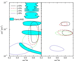
In left panel of Fig. 2 we present the allowed regions in neutrino parameter space that follows from our analysis. The straight line corresponds to the allowed region with 95% C.L., with no fluctuation, when only the solar neutrino data is taken into account.
Our KamLAND analysis results in the following best fit point:
∆m2= 7.24·10−5eV2, tan2θ= 0.52. (19)
The filled areas represent the allowed regions that comes from the KamLAND analysis, also with 95% C.L.
The concordance between the KamLAND and the so-lar neutrino data analysis is excellent. The allowed regions overlap, creating two island in the parameter space, that is called the high-LMA and low-LMA, as can be seen in Fig. 2. In presence of the random perturbations, the allowed re-gions are displaced to smaller mixing angles and∆m2. This can be understood by looking at Fig. 1. By increasing the size of random fluctuations, the survival probability approa-ches the value of0.5, which can be mimicked by an incre-ase of mixing angle. Also, the distortion of spectrum that characterizes transition between resonant and non-resonant conversion is pushed to smaller values of∆m2/4E, which reflects in a displacement of allowed regions to smaller va-lues of∆m2.
0.2 0.4 0.6 0.8
sin2
2θ
10−5 10−4 10−3
∆
m
2 (eV
2)
ξ=0%
ξ=2%
ξ=4%
ξ=8%
0.2 0.4 0.6 0.8 1
sin2
2θ
KamLAND
Figure 2. LMA region for different values of the perturbation am-plitude, at 95% C.L. for several values of the perturbation ampli-tude,ξ= 0%(solid line), forξ= 2%(long dashed line),ξ= 4% (dashed line) andξ = 8%(dotted line). We also present the al-lowed region for KamLAND spectral data, for the same C.L.. In the right-handed side of the figure, the combined analysis of both solar neutrino and KamLAND observations is shown.
Since KamLAND experiment is insensitive to fluctua-tions in solar density, in the combined analysis the Kam-LAND data prevents the allowed regions to displace in
∆m2. But for high enough values of the size of random fluc-tuations, a new region of compatibility between KamLAND and solar neutrino data appears, around∆m2∼2×10⁻⁵.
We call this region “very-low LMA”.
In Fig. 3 it is shownχ2as a function of the perturbation amplitude, minimized in∆m2andsin22θ. We can see that even for high values of the perturbation amplitude we still can have a viable solution. We notice that even in a noisy scenario the compatibility of solar neutrino and KamLAND results is still good. In fact, although the absolute best fit of the analysis lies on the non-noise picture whereξ = 0, we observe that(χ2−χ2
min)<4for5%< ξ <8%, showing
a new scenario of compatibility.
0 2 4 6 8 10
ξ (%) 70
72 74 76 78 80
χ
2
Figure 3.χ2as a function ofξ, the perturbation amplitude, where
References
[1] KamLAND collaboration, K. Eguchi et al., Phys. Rev. Lett.
90, 021802 (2003).
[2] L. Wolfenstein, Phys. Rev. D17, 2369 (1978).
[3] S.P. Mikheyev and A. Yu. Smirnov, Yad. Fiz. 42, 1441 (1985) [Sov. J. Nucl. Phys. 42, 913 (1985)], Nuovo Cimento C9, 17 (1986); S.P. Mikheyev and A. Yu. Smirnov, ZHTEF 91 (1986) [Sov. Phys. JETP 64, 4 (1986)].
[4] P. C. de Holanda and A. Yu. Smirnov, hep-ph/0309299, ac-cepted to be published at Astropart. Phys.
[5] P. C. de Holanda and A. Yu. Smirnov, Journ. of Cosm. and Astropart. Phys. 02, 001 (2003).
[6] M.M. Guzzo, A. Masiero and S. T. Petcov, Phys. Lett. B 260, 154 (1991).
[7] E. Roulet, Phys. Rev. D 44, 935 (1991).
[8] S. Bergmann, M.M. Guzzo, P.C. de Holanda, P. Krastev and H. Nunokawa, Phys. Rev. D 62, 073001 (2000).
[9] J. Schechter and J. W. F. Valle, Phys. Rev. 24, 1883 (1981); ibid. 25, 283 (1982).
[10] C. S. Lim and W. J. Marciano, Phys. Rev. 37, 1368 (1988).
[11] E. Kh. Akhmedov, Sov. J. Nucl. Phys. 48, 382 (1988); Phys. Lett. B 213, 64 (1988).
[12] M. M. Guzzo and H. Nunokawa, Astropart. Phys. 12, 87 (1999).
[13] M. Gasperini, Phys. Rev. D 38, 2635 (1988); ibid. 39, 3606 (1989).
[14] A. M. Gago, H. Nunokawa and R. Zukanovich Funchal, Phys. Rev. Lett. 84, 4035 (2000); Nucl. Phys. (Proc. Suppl.) B 100, 68 (2001).
[15] A. Halprin and C. N. Leung, Phys. Rev. Lett. 67, 1833 (1991).
[16] S. W. Mansour and T. K. Kuo, Phys. Rev. D 60, 097301 (1999); A. Raychaudhuri and A. Sil, hep-ph/0107022.
[17] Y. Fukuda et. al. [Super-Kamiokande Collaboration], Phys. Rev. Lett. 81, 1562 (1998).
[18] CHOOZ Collaboration, M. Apollonio et al., Phys.Lett. B466, 415 (1999); Eur. Phys. J. , C 27, 331 (2003).
[19] P. C. de Holanda and A. Yu. Smirnov, hep-ph/0307266.
[20] J. Barranco, O.G. Miranda, T.I. Rashba, V.B. Semikoz, J.W.F. Valle, Phys. Rev. D 66 093009 (2002); O. G. Mirana, T. I. Rashba, A. I. Rez, J. W. F. Valle, hep-ph/0311014.
[21] P.A. Sturrock, Astrophys. J. 594, 1102 (2003).
[22] J. Yoo et al. [Super-Kamiokande collaboration], Phys. Rev.
D 68 092002 (2003);
[23] P. A. Sturrock, hep-ph/0309239; D.O. Caldwell, P.A. Stur-rock, hep-ph/0309191.
[24] H. Nunokawa, A. Rossi, V. B. Semikoz, J. W. F. Valle, Nucl. Phys. B 472, 495 (1996).
[25] S. Turck-Chi´eze and I. Lopes, Ap. J 408 (1993) 346; S. Turck-Chi´eze et al., Phys. Rep. 230 (1993) 57.
[26] P. Kumar, E. J. Quataert and J. N Bahcall, Astrophys. Journ.
458, L83 (1996).
[27] P. Bamert, C. P. Burgess and D. Michaud, Nucl. Phys. B 513, 319 (1998).
[28] C. Burgess et al., hep-ph/0209094 v1.
[29] C. P. Burgess, N. S. Dzhalilov, T. I. Rashba, V. B. Semikoz and J. W. F. Valle, M.N.R.A.S. (to appear), astro-ph/0304462.
[30] N. Reggiani, M. M. Guzzo and P.C. de Holanda, Braz. J. Phys. 33, 767 (2003). M. M. Guzzo, P. C. de Holanda, N. Reggiani, Eur.Phys.J.C 25, 459 (2002); N. Reggiani, M. M. Guzzo, J.H. Colonia and P. C. de Holanda, Eur. Phys. J. C 12, 263 (2000);
[31] H. Nunokawa, A. Rossi, V. B. Semikoz, J. W. F. Valle, hep-ph/9602307.
[32] B. T. Cleveland et al., Astroph. J. 496, 505 (1998).
[33] SAGE collaboration, J.N. Abdurashitov et al. Zh. Eksp. Teor. Fiz. 122, 211 (2002) [J. Exp. Theor. Phys. 95, 181 (2002)], astro-ph/0204245; V. N. Gavrin, Talk given at the VIIIth In-ternational conference on Topics in Astroparticle and Under-ground Physics (TAUP 03), Seattle, Sept. 5 - 9, 2003.
[34] GALLEX collaboration, W. Hampel et al., Phys. Lett. B 447, 127 (1999).
[35] GNO Collaboration, E. Belotti, Talk given at the VIIIth In-ternational conference on Topics in Astroparticle and Under-ground Physics (TAUP 03), Seattle, Sept. 5 - 9, 2003.
[36] Super-Kamiokande collaboration, S. Fukuda et al., Phys. Rev. Lett. 86, 5651 (2001); Phys. Rev. Lett. 86, 5656 (2001), Phys. Lett. B 539, 179 (2002).
[37] Super-Kamiokande collaboration, M. B. Smy et al., hep-ex/0309011.
[38] SNO collaboration, Q. R. Ahmad et al.; ibidem 87, 071301 (2001); ibidem 89, 011301 (2002); ibidem 89, 011302 (2002).
[39] SNO collaboration (Q. R. Ahmad et al.), nucl-ex/0309004.
[40] “HOWTO use the SNO salt flux results”, website: www.sno.phy.queensu.ca .
[41] J. N. Bahcall, M.H. Pinsonneault and S. Basu, Astrophys. J.