Apriori-based algorithms for
k
m
-anonymizing
trajectory data
Giorgos Poulis
∗, Spiros Skiadopoulos
∗, Grigorios Loukides
∗∗, Aris
Gkoulalas-Divanis
∗∗∗∗University of Peloponnese, Email:{poulis,spiros}@uop.gr ∗∗Cardiff University, Email: [email protected] ∗∗∗IBM Research - Ireland, Email: [email protected]
Abstract. The proliferation of GPS-enabled devices (e.g., smartphones and tablets) and location-based social networks has resulted in the abundance of trajectory data. The publication of such data opens up new directions in analyzing, studying and understanding human behavior. However, it should be performed in a privacy-preserving way, because the identities of individuals, whose movement is recorded in trajectories, can be disclosed even after removing identifying information. Existing trajectory data anonymization approaches offer privacy but at a high data utility cost, since they either do not produce truthful data (an important requirement of several applications), or are limited in their privacy specification component. In this work, we propose a novel approach that overcomes these shortcomings by adaptingkm
-anonymity to trajectory data. To realize our approach, we develop three efficient and effective anonymization algorithms that are based on the apriori prin-ciple. These algorithms aim at preserving different data characteristics, including location distance and semantic similarity, as well as user-specified utility requirements, which must be satisfied to en-sure that the released data can be meaningfully analyzed. Our extensive experiments using synthetic and real datasets verify that the proposed algorithms are efficient and effective at preserving data utility.
Keywords. privacy, anonymity, trajectories, spatial data,km
-anonymity, utility constraints
1
Introduction
The widespread adoption of GPS-enabled smartphones and location-based social network-ing applications, such as Foursquare (https://foursquare.com), opens up new op-portunities in understanding human behaviour through the analysis of collected mobility data. However, the publication of these data, which correspond to trajectories of personal movement (i.e., ordered lists of locations visited by individuals), can lead toidentity disclo-sure, even if directly identifying information, such as names or SSN of individuals, is not published [33].
The values that, in combination, may lead to identity disclosure are calledquasi-identifiers
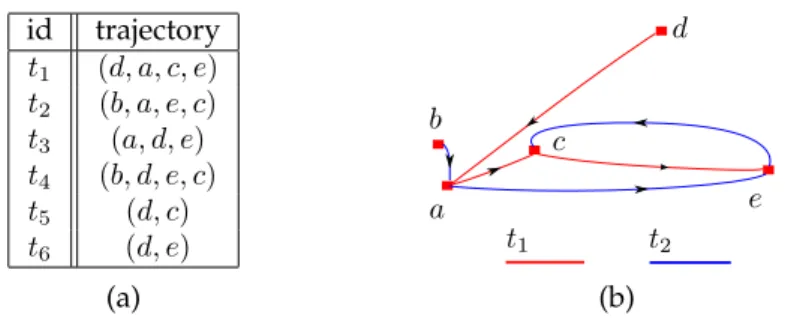
id trajectory
t1 (d, a, c, e)
t2 (b, a, e, c)
t3 (a, d, e)
t4 (b, d, e, c)
t5 (d, c)
t6 (d, e)
(a)
a b
c
d
e
t2
t1
(b)
Figure 1: (a) the original databaseT (b) visual representation of trajectoriest1andt2 checked in at locationsaandd, he cannot associate Mary with her record (trajectory), as both trajectoriest1andt3 include the locationsaandd. But if John knew that Mary first checked in at locationdand then ata, he can uniquely associate Mary with the trajectory
t1.
This example highlights not only the need to transform a set of user trajectories T to prevent identity disclosure based on partial location knowledge held by attackers, but also the difference from well-studied set-valued data anonymity models, likekm-anonymity [36] and privacy-constrained anonymization [18,24]. In these models, value ordering is not significant; thus, records are represented as unordered sets of items. For instance, if an attacker knows that someone checked in first at the locationcand then ate, they could uniquely associate this individual with the recordt1(Figure1b). On the other hand, ifT was a set-valued dataset, three records, namelyt1,t2andt4, would have the itemscande. Thus, the individual’s identity is “hidden” among3records. Consequently, for any set ofn
items in a trajectory, there aren!possible quasi-identifiers.
This difference makes preventing identity disclosure in trajectory data publishing more challenging, as the number of potential quasi-identifiers is drastically increased. Exist-ing methods operate either by anonymizExist-ing (i) each trajectory as a whole, thereby not assuming any specific background knowledge of attackers [1, 2,26, 29], or (ii) parts of trajectories, thereby considering attackers who aim to re-identify individuals based on spe-cific locations [35,39]. The first category of methods are based on clustering and
pertur-bation[1,2,29], while the second category employsgeneralization and suppressionof
quasi-identifiers [27,39,28,35]. The main drawback of clustering-based methods is that they may lose information about the direction of movement of co-clustered trajectories and cause ex-cessive information loss, due to space translation. Moreover, applying perturbation may create data that are nottruthfuland cannot be used in several applications [14]. Similarly, existing generalization-and-suppression based methods [27,39,28,35] have the following limitations. First, they assume that quasi-identifiers are known to the data publisher prior to anonymization [35,39], or that any combination of locations can act as a quasi-identifier [27]. Second, they require a location taxonomy to be specified by data publishers [28] based on location semantics. However, such a taxonomy may not exist, or may not accurately re-flect the distance between locations. In both cases, the anonymized data will be highly distorted. Last, some approaches assume that each location can be classified as either sen-sitive or non-sensen-sitive [28]. In practice, however, this assumption may not hold, as location sensitivity usually depends on context (e.g., visiting a hospital may be considered as sensi-tive for a patient, but not for a doctor).
by employingperturbation. Specifically, they release a noisy summary of the original data that can be used in specific analytic tasks, such as frequent sequential pattern mining [3]. While being able to offer strong privacy guarantees, these approaches do not preserve data truthfulness, since they rely on perturbation.
1.1
Contributions
In this work, we propose a novel approach for publishing trajectory data, in a way that pre-vents identity disclosure, and three effective and efficient algorithms to realize it. Specifi-cally, our work makes the following contributions.
First, we adaptkm-anonymity [35,36] to trajectory data.km-anonymity is a privacy model that was proposed to limit the probability of identity disclosure in transaction data pub-lishing. The benefit of this model is that it does not require detailed knowledge of quasi-identifiers, or a distinction between sensitive and non-sensitive information, prior to data publishing.
Second, we develop three algorithms for enforcingkm-anonymity on trajectory data. These algorithms generalize data in an apriori-like fashion (i.e., apply generalization to increas-ingly larger parts of trajectories) and aim at preserving different aspects of data utility. Our first algorithm, called SEQANON, appliesdistance-basedgeneralization, effectively creating generalized trajectories with locations that are close in proximity. For instance, SEQANON would favor generalizingatogether withb, becausebis the closest location toa, as can be seen in Fig. 1b. SEQANONdoes not require a location taxonomy and aims at preserving the distance between original locations. Thus, it should be used when accurate semantic information about locations is not available1. Clearly, however, the presence of accurate, se-mantic location information should also be exploited, as it can help the preservation of data utility. For example, assume thataandcrepresent the locations of restaurants, whereasb
experiments verify that our approach is able to anonymize trajectory data, under various privacy and utility requirements, with a low level of information loss. In addition, they show that our algorithms are fast and scalable, due to the use of the apriori principle.
1.2
Organization
The rest of the paper is organized as follows. Section2discusses related work. Section 3presents some preliminary concepts related to trajectory data anonymization, as well as the privacy and utility objectives of our algorithms. Section4presents our anonymization algorithms, and Section5an experimental evaluation of them. Last, we conclude the paper in Section6.
2
Related work
Privacy-preserving trajectory data publishing has attracted significant attention, due to the pervasive use of location-aware devices and location-based social networks, which led to a tremendous increase in the volume of collected data about individuals [4]. One of the main concerns in trajectory data publishing is the prevention of identity disclosure, which is the objective of thek-anonymity privacy model [33,34]. k-anonymity prevents identity disclosure by requiring at least krecords of a dataset to have the same values over QI. Thus, ak-anonymous dataset upperbounds the probability of associating an individual with their record by 1k. To enforce k-anonymity most works [15,20, 21,23,32] employ
generalization, which replaces a QI value with a more general but semantically consistent
value, orsuppression, which removes QI values prior to data publishing.
k-anonymity has been considered in the context of publishing user trajectories, leading to several trajectory anonymization methods [4]. As mentioned in Section1, these methods operate by anonymizing either entire trajectories [1,2,26], or parts of trajectories (i.e., se-quences of locations) that may lead to identity disclosure [35,39]. In the following, we dis-cuss the main categories of trajectory anonymization works, as well as how our approach differs from them.
2.1
Clustering and perturbation
Methods based on clustering and perturbation are applied to time-stamped trajectories. They operate by grouping original trajectories into clusters (cylindrical tubes) of at leastk
trajectories, in a way that each trajectory within a cluster becomes indistinguishable from the other trajectories in the cluster. One such method, calledNWA [1], enforces (k, δ) -anonymity to anonymize user trajectories by generating cylindrical volumes of radiusδ
that contain at leastk trajectories. Each trajectory that belongs to an anonymity group
(cylinder), generated by NWA, is protected from identity disclosure, due to the other
and then permutes the locations in each cluster to enforce privacy. The experimental eval-uation in [11] demonstrates thatSwapLocationsis significantly more effective at preserving data utility thanNWA[1]. Finally, Lin et al. [22] guaranteesk-anonymity of published data, under the assumption that road-network data are public information. Their method uses clustering-based anonymization, protecting from identity disclosure.
Contrary to the methods of [1,2,11,22], our work (a)does not consider time-stamped trajectories, and(b)applies generalization to derive an anonymized dataset.
2.2
Generalization and suppression
Differently to the methods of Section2.1, this category of methods considers attackers with background knowledge on ordered sequences of places of interest (POIs) visited by specific individuals. Terrovitis et al. [35] proposed an approach to prohibit multiple attackers, each knowing a different set of POIs, from associating these POIs to fewer thankindividuals in the published dataset. To achieve this, the authors developed a suppression-based method that aims at removing the least number of POIs from user trajectories, so that the remaining trajectories arek-anonymous with respect to the knowledge of each attacker.
Yarovoy et al. [39] proposed ak-anonymity based approach for publishing user trajecto-ries by considering time as a quasi-identifier and supporting privacy personalization. Un-like previous approaches that assumed that all users share a common quasi-identifier, [39] assumes that each user has a different set of POIs and times requiring protection, thereby enabling each trajectory to be protected differently. To achievek-anonymity, this approach uses generalization and creates anonymization groups that are not necessarily disjoint.
A recent approach, proposed by Monreale et al. [27], extends thel-diversity principle to trajectories by assuming that each location is either nonsensitive (acting as a QI) or sensi-tive. This approach appliesc-safety to prevent attackers from linking sensitive locations to trajectories with a probability greater thanc. To enforcec-safety, the proposed algorithm applies generalization to replace original POIs with generalized ones based on a location taxonomy. If generalization alone cannot enforcec-safety, suppression is used.
Assuming that each record in a dataset is comprised of a user’s trajectory and user’s sensi-tive attributes, Chen et al. [8] propose the(K, C)L-privacy model. This model protects from identity and attribute linkage by employing local suppression. In this paper, the authors assume that an adversary knows at mostLlocations of a user’s trajectory. Their model guarantees that a user is indistinguishable from at leastK−1users, while the probability of linking a user to his/her sensitive values is at mostC.
Contrary to the methods of [8,27,35,39], our work(a)assumes that an attacker may know up tomuser locations, which is a realistic assumption in many applications, and(b)does not classify locations as sensitive or nonsensitive, which may be difficult in some domains [36].
2.3
Differential privacy
Recently, methods for enforcing differential privacy [12] on trajectory data have been pro-posed [5,7,9]. The objective of these methods is to release noisy data summaries that are effective at supporting specific data analytic tasks, such as count query answering [7,9] and frequent pattern mining [5]. To achieve this, the method in [9] uses acontext-free,taxonomy
The method proposed in [7] was shown to be able to generate summaries that permit highly accurate count query answering. This method, referred to as NGRAMS, works in three steps. First, it truncates the original trajectory dataset by keeping only the firstℓmax locations of each trajectory, whereℓmaxis a parameter specified by data publishers. Larger
ℓmax values improve efficiency but deteriorate the quality of the frequencies, calculated during the next step. Second, it uses the truncated dataset to compute the frequency of
n-grams(i.e., all possible contiguous parts of trajectories that are comprised of1, or2, ... ,
ornlocations). Third, this method constructs a differentially private summary by inserting calibrated Laplace noise [12] to the frequencies of n-grams.
Contrary to the methods of [5,7,9], our work publishes truthful data at a record (individ-ual user) level, which is required by many data analysis tasks [24]. That is, our work retains the number of locations in each published trajectory and the number of published trajec-tories in the anonymized dataset. Furthermore, our method is able to preserve data utility significantly better than these methods, as shown in our extensive experiments. Thus, our approach can be used to offer a better privacy/utility trade-off than the methods of [5,7,9].
3
Privacy and utility objectives
In this section, we first define some preliminary concepts that are necessary to present our approach, and then discuss the privacy and utility objectives of our anonymization algorithms.
3.1
Preliminaries
LetLbe a set of locations (e.g., points of interest, touristic sites, shops). A trajectory rep-resents one or more locations inLand the order in which these locations are visited by a moving object (e.g., individual, bus, taxi), as explained in the following definition.
Definition 1. Atrajectorytis an ordered list of locations(l1, . . . , ln), whereli ∈ L,1 ≤i ≤n.
Thesizeof the trajectoryt= (l1, . . . , ln), denoted by|t|, is the number of its locations, i.e.,|t|=n. Note that, in our setting, a location may model points in space. A part of a trajectory, which is formed by removing some locations while maintaining the order of the remaining locations, is asubtrajectoryof the trajectory, as explained below.
Definition 2. A trajectorys = (λ1, . . . , λν)is asubtrajectory ofor iscontained intrajectory
t = (l1, . . . , ln), denoted bys ⊑ t, if and only if|s| ≤ |t|and there is a mapping f such that
λ1=lf(1), . . . , λν =lf(ν)andf(1)<· · ·< f(ν).
For instance, the trajectory(a, e)is a subtrajectory of (or contained in) the trajectoryt1=
(d, a, c, e)in Figure1. Clearly,(a, e)can be obtained fromt1by removingdandc.
Definition 3. Given a set of trajectoriesT, thesupportof a subtrajectorys, denoted bysup(s,T),
is defined as the number of distinct trajectories inT that contains.
In other words, the support of a subtrajectorysmeasures the number of trajectories in a dataset thatsis contained in. For example, for the dataset in Figure1a, we havesup((a, e),T) = 3. Note that the support does not increase when a subtrajectory is contained multiple times in a trajectory. For instance,sup((a, e),{(a, e, b, a, e)}) = 1. Naturally, by considering loca-tions as unary trajectories, the support can also be measured for the localoca-tions of a dataset.
Definition 4. A set of trajectories T iskm-anonymousif and only if every subtrajectory sof
every trajectoryt ∈ T, which containsmor fewer locations (i.e.,|s| ≤m), is contained in at least
kdistinct trajectories ofT.
Definition4ensures that an attacker who knows any subtrajectorysof sizemof an indi-vidual, cannot associate the individual to fewer thanktrajectories (i.e., the probability of identity disclosure, based ons, is at mostk1). The privacy parameterskandmare specified by data publishers, according to their expectations about adversarial background knowl-edge, or certain data privacy policies [18,35,36].
The following example illustrates a dataset that satisfieskm-anonymity.
Example 1. Consider the trajectory dataset that is shown in Figure1a. This dataset is21
-anony-mous, because every location (i.e., subtrajectory of size1) appears at least2times in it. This dataset
is also13-anonymous, because every subtrajectory of size3appears only once in it. However, the
dataset is not22-anonymous, as the subtrajectory(d, a)is contained only in the trajectoryt1.
Note that, unlikek-anonymity, the km-anonymity model assumes that an attacker pos-sesses background knowledge about subtrajectories, which are comprised of at mostm
locations. That is, an attacker knows at mostmlocations that are visited by an individual, in a certain order. Clearly,mcan be set to any integer in[0,max{|t|
t ∈ T }]. Settingm
to0corresponds to the trivial case, in which an attacker has no background knowledge. On the other hand, settingmtomax{|t|
t∈ T }, can be used to guard against an attacker
who knows the maximum possible subtrajectory about an individual (i.e., that an indi-vidual has visited all the locations in their trajectory, and the order in which they visited these locations). In this case,km-anonymity “approximates”k-anonymity, but it does not provide the same protection guarantees against identity disclosure. This is becausekm -anonymity does not guarantee protection from attackers who know that an individual has visitedexactlythe locations, contained in a subtrajectory of sizem. For example, assume that a dataset is comprised of the trajectories{(a, d, e),(a, d, e),(a, d)}. The dataset satisfies 23-anonymity, hence it prevents an attacker from associating an individual with any of the subtrajectories(a, d),(a, e), and(d, e). However, the dataset is not2-anonymous, hence an attacker who knows that an individual has visited exactly the locationsaandd, in this order, can uniquely associate the individual with the trajectory(a, d).
The km-anonymity model is practical in several applications, in which it is extremely difficult for attackers to learn a very large number of user locations [35]. However, km -anonymity does not guarantee that all possible attacks, based on background knowledge, will be prevented. For example,km-anonymity is not designed to preventcollaborative
at-tacks, in which(i)two or more attackers combine their knowledge in order to re-identify
an individual, or(ii)an attacker possesses background knowledge about multiple trajec-tories inT. Such powerful attack schemes can only be handled within stronger privacy principles, such as differential privacy (see Section2). However, applying these principles usually results in significantly lower data utility, compared to the output of our algorithms, as shown in our experiments. In addition, as we do not deal with time-stamped trajectories, time information is not part of our privacy model. In the case of time-stamped trajectory data publishing, time information can be used by attackers to perform identity disclosure, and privacy models to prevent this are the focus of [8,39]. For the same reason, we do not deal with attacks that are based on both time and road-network information (e.g., the
inference route problem[22]). These attacks can be thwarted using privacy models, such as
strictk-anonymity [22].
Definition 5. Ageneralized location{l1, . . . , lv} is defined as a set of at least two locations
l1, . . . , lv ∈ L.
Thus, a generalized location is the result of replacing at least two locations inLwith their set. Ageneralized locationis interpreted as exactly one of the locations mapped to it. For example, the generalized location{a, b} may be used to replace the locationsaand b in Figure1a. This generalized location will be interpreted asaorb. Therefore, if a trajectory
t′ in an anonymized versionT′ofT contains a generalized location{l
1, . . . , lv}, then the
trajectorytinT contains exactly one of the locationsl1, . . . , lv.
To enforcekm-anonymity, we either replace a locationl with a generalized location that containsl, or leavel intact. Thus, ageneralized trajectoryt′ is an ordered list of locations
and/or generalized locations. Thesizeoft′, denoted by|t′|, is the number of elements of t′. For instance, a generalized trajectoryt′ = ({a, b}, c) is comprised of one generalized
location{a, b}and a locationc, and it has a size of2.
We are interested in generalization transformations that produce a transformed dataset
T′ by distorting the original dataset T as little as possible, A common way to measure
the distortion of a transformation is to measure thedistancebetween the original and the transformed dataset [29,35,39]. In our case, the distance between the original and the anonymized dataset is defined as theaverageof the distances of their corresponding trajec-tories. In turn, the distance between the initial and the anonymized trajectory is defined as
theaverageof the distance between their corresponding locations.
The following definition illustrates how the distance between locations, trajectories, and datasetsT andT′can be computed.
Definition 6. Letl be a location that will be generalized to the generalized location{l1, . . . , lv}.
Thelocation distancebetweenland{l1, . . . , lv}, denoted byDloc(l,{l1, . . . , lv}), is defined as:
Dloc(l,{l1, . . . , lv}) = avg
d(l, li)|1≤i≤v
wheredis the Euclidean distance. Thetrajectory distancebetweent= (l1, . . . , ln)and its
gener-alized counterpartt′= (l′
1, . . . , l′n), denoted byDtraj(t, t′), is defined as:
Dtraj(t, t′) = avgDloc(li, li′)|1≤i≤n
Finally, thetrajectory dataset distancebetweenT ={t1, . . . , tu}and its generalized counterpart
T′ = {t′
1, . . . , t′u}(where the trajectoryti is generalized to trajectoryt′i,1 ≤i ≤u), denoted by
D(T,T′), is defined as:
D(T,T′) = avg
Dtraj(ti, t′i)|1≤i≤u
For example, leta,a1,a2andbbe locations and letd(a, a1) = 1andd(a, a2) = 2. If location
ais generalized to the generalized location{a, a1, a2}the location distanceDloc(a,{a, a1, a2}) = (0 + 1 + 2)/3 = 1. Also, if trajectory(a, b)is generalized to({a, a1, a2}, b)the trajectory dis-tanceDtraj((a, b),({a, a1, a2}, b)) = (1 + 0)/2 = 1/2.
Note that the distances in Definition6can be normalized by dividing each of them with the maximum distance between locations inT.
3.2
Problem statement
of data utility that data publishers may want to preserve. To account for this, we have developed three anonymization algorithms, namely SEQANON, SD-SEQANON, and U-SEQANON, which generalize locations in different ways.
The SEQANONalgorithm aims at generalizing together locations that are close in proxim-ity. The distance between locations, in this case, is expressed based on Definition6. Thus, the problem that SEQANONaims to solve can be formalized as follows.
Problem 1. Given an original trajectory datasetT, construct akm-anonymous version T′ ofT
such thatD(T,T′)is minimized.
Note that Problem1is NP-hard (the proof follows easily from observing that Problem1 contains the NP-hard problem in [35] as a special case), and that SD-SEQANONis a heuris-tic algorithm that may not find an optimal solution to this problem.
The SD-SEQANONalgorithm considers both the distance and the semantic similarity of locations, when constructing generalized locations. Thus, it exploits the availability of se-mantic information about locations to better preserve data utility. Following [27], we as-sume that the semantic information of locations is provided by data publishers, using a location taxonomy. The leaf-level nodes in the taxonomy correspond to each of the loca-tions of the original dataset, while the non-leaf nodes represent more general (abstract) location information.
Given a location taxonomy, we define the notion ofsemantic dissimilarityfor a generalized location, as explained in the following definition. A similar notion of semantic dissimilarity, for relational values, was proposed in [38].
Definition 7. Letl′ ={l
1, . . . , lv}be a generalized location andHbe a location taxonomy. The
semantic dissimilarityforl′is defined as:
SD(l′) = CCA({l1, . . . , lv})
|H|
whereCCA({l1, . . . , lj})is the number of leaf-level nodes in the subtree rooted at the closest
com-mon ancestor of the locations{l1, . . . , lv}in the location taxonomyH, and|H|is the total number
of leaf-level nodes inH.
Thus, locations that belong to subtrees with a small number of leaves are more semanti-cally similar. Clearly, theSDscores for generalized locations that contain more semanti-cally similar locations are lower.
Example 2. An example location taxonomy is illustrated in Figure2. The leaf-level nodesatoe represent the locations (i.e., specific restaurants and coffee houses), while the non-leaf nodes represent
the general conceptsRestaurantsand Coffee shops. We also haveCCA({a, c, e}) = 3, as the
subtree rooted atRestaurantshas three leaf-level nodes, and|H|= 5, as the taxonomy in Figure2
has 5 leaf-level nodes. Thus, the semantic dissimilarity for the generalized location{a, c, e}, denoted
withSD({a, c, e}), is 3
5 = 0.6. Similarly, we can computeSD({a, d}) =
5
5 = 1, which is greater
thanSD({a, c, e})because aanddare more semantically dissimilar (i.e., restaurants and coffee
shops, instead of just restaurants).
We now define the criteria that are used by the SD-SEQANONalgorithm to capture both the distance and semantic similarity between locations, trajectories, and datasetsT andT′.
Any
Coffee shops Restaurants
b d a c e
Figure 2: A location taxonomy
Definition 8. Let l be a location that will be generalized to l′ = {l
1, . . . , lv}. Thecombined
location distancebetweenlandl′, denoted byC
loc(l, l′), is defined as:
Cloc(l, l′) = avgd(l, li)·SD(l′)|1≤i≤v ,whereSD(l′)takes values in(0,1]
whered is the Euclidean distance andSDis the semantic dissimilarity. Note that the above
for-mula is a conventional weighted-forfor-mula, where similarity and distance are combined into the
Cloc(l, l′). Thus, the combined objective is then optimized by the single-objective optimization
met-ricCloc(l, l′). Using conventional weighted-formulas is an effective approach for addressing
multi-objective optimization problems, as discussed in [13]. Thecombined trajectory distancebetween
t= (l1, . . . , ln)and its generalized counterpartt′ = (l1′, . . . , l′n), denoted byCtraj(t, t′), is defined
as:
Ctraj(t, t′) = avg
Cloc(li, l′i)|1≤i≤n
Finally, thecombined trajectory dataset distancebetweenT ={t1, . . . , tu}and its generalized
counterpartT′ ={t′
1, . . . , t′u}(where the trajectorytiis generalized to trajectoryt′i,1 ≤i ≤u),
denoted byC(T,T′), is defined as:
C(T,T′) = avg
Ctraj(ti, t′i)|1≤i≤u
We now define the problem that the SD-SEQANONalgorithm aims to solve, as follows.
Problem 2. Given an original trajectory datasetT, construct akm-anonymous version T′ ofT such thatC(T,T′)is minimized.
Note that Problem2 can be restricted to Problem 1, by allowing only instances where
SD(l′) = 1, for each generalized locationl′ that is contained in a trajectory ofT′. Thus,
Problem2is also NP-hard. The SD-SEQANONalgorithm aims to derive a (possibly sub-optimal) solution to Problem2by taking into account both the distance and the semantic similarity of locations, when constructing generalized locations.
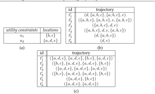
utility constraints locations
u1 {b, c}
u2 {a, d, e}
(a)
id trajectory
t′
1 (d,{a, b, c},{a, b, c}, e)
t′
2 ({a, b, c},{a, b, c}, e,{a, b, c})
t′
3 ({a, b, c}, d, e)
t′4 ({a, b, c}, d, e,{a, b, c})
t′
5 (d,{a, b, c})
t′
6 (d, e)
(b)
id trajectory
t′
1 ({a, d, e},{a, d, e},{b, c},{a, d, e})
t′
2 ({b, c},{a, d, e},{a, d, e},{b, c})
t′
3 ({a, d, e},{a, d, e},{a, d, e})
t′
4 ({b, c},{a, d, e},{a, d, e},{b, c})
t′
5 ({a, d, e},{b, c})
t′
6 ({a, d, e},{a, d, e})
(c)
Figure 3:(a)An example utility constraint setU. (b)A22-anonymous datasetT′that does
not satisfy the utility constraint setU.(c)A22-anonymous datasetT′that satisfiesU.
Definition 9. Autility constraintuis a set of locations{l1, . . . , lv}, specified by data publishers.
Autility constraint setU ={u1, . . . , up}is a partition of the set of locationsL, which contains
all the specified utility constraintsu1, . . . , up.
Definition 10. Given a utility constraint setU = {u1, . . . , up}, a generalized datasetT′ that
contains a set of generalized locations{l′
1, . . . , l′n}, and a parameterδ,U is satisfied if and only if
(i)for each generalized locationl′ ∈ {l′
1, . . . , l′n}, and for each utility constraintu∈ U,l′ ⊆uor
l′∩u=∅, and(ii)at mostδ%of the locations inLhave been suppressed to produceT′, whereδis
a parameter specified by data publishers.
The first condition of Definition10limits the maximum amount of generalization each lo-cation is allowed to receive, by prohibiting the construction of generalized lolo-cations whose elements (locations) span multiple utility constraints. The second condition ensures that the number of suppressed locations is controlled by a threshold. When both of these con-ditions hold, the utility constraint setU is satisfied. Note that we assume that the utility constraint set is provided by data publishers, e.g., using the method in [24]. The example below illustrates Definitions9and10.
Example 3. Consider the utility constraint setU ={u1, u2}, shown in Figure3a, and assume that
δ= 5. The dataset, shown in Figure3b, does not satisfyU, because the locations in the generalized
location{a, b, c} are contained in both u1 and u2. On the other hand, the dataset in Figure3c
satisfiesU, because the locations of every generalized location are all contained inu1.
type of locations, such ascoffee shopsandbus stationswhen data recipients are coffee shops owners and public transport authorities, respectively. The second example comes from the healthcare domain, and it is related to publishing the locations (e.g., healthcare institutions, clinics, and pharmacies) visited by patients [25]. To support medical research studies, it is important that the published data permit data recipients to accurately count the number of trajectories (or equivalently the number of patients) that are associated with specific loca-tions, or types of locations.
Observe that the number of trajectories that contain a generalized locationl′ = (l1, . . . , ln), in the generalized datasetT′, is equal to the number of trajectories that containat leastone
of the locationsl1, . . . , ln, in the original datasetT. This is because a trajectoryt∈ T that contains at least one of these locations corresponds to a trajectoryt′ ∈ T′ that contains l′. Thus, the number of trajectories inT that contain any location in a utility constraint u ∈ U can be accurately computed from the generalized datasetT′, whenU is satisfied,
as no other location will be generalized together with the locations inu. Therefore, the generalized data that satisfyUwill be practically useful in the aforementioned applications.
We now define the problem that U-SEQANONaims to solve, as follows.
Problem 3. Given an original trajectory datasetT, a utility constraint setU, and parametersk,
mand δ, construct akm-anonymous versionT′ ofT such thatD(T,T′)is minimized andU is
satisfied with at mostδ%of the locations ofT being suppressed.
Thus, a solution to Problem 3needs to satisfy the specified utility constraints, without suppressing more thanδ%of locations, and additionally incur minimum information loss. Note that Problem3is NP-hard (it can be restricted to Problem1, by allowing only instances whereU contains an single utility constrained with all locations inLandδ= 100) and that U-SEQANONis a heuristic algorithm that may not solve Problem3optimally.
4
Anonymization algorithms
In this section, we present our SEQANON, SD-SEQANON, and U-SEQANON anonymiza-tion algorithms, which aim at solving Problems1,2, and3, respectively.
4.1
The S
EQA
NONalgorithm
The pseudocode of the SEQANON algorithm is illustrated in Algorithm SEQANON. The algorithm takes as input a trajectory datasetT, and the anonymization parameterskand
m, and returns thekm-anonymous counterpartT′ ofT. The algorithm employs the
apri-ori principle and works in a bottom up fashion. Initially, it considers and generalizes the subtrajectories of size1 (i.e., single locations) in T which have low support. Then, the algorithm continues by progressively increasing the size of the subtrajectories it considers. In more detail, SEQANONproceeds as follows. First, it initializes T′ (Step1). Then, in
Steps2–8, it considers subtrajectories of size up tom, iteratively. Specifically, in Step3, it computes the setS, which contains all subtrajectories inT that have sizei(i.e., that have
ilocations) and support lower thank(i.e.,sup(s,T′) < k). S
Algorithm: SEQANON
Input: A datasetT and anonymization parameterskandm
Output: Akm
-anonymous datasetT′corresponding toT
1 T′:=T // Initialize output 2 fori:= 1tomdo
3 LetSbe the set of subtrajectoriessofT with sizeisuch thatsup(s,T′)< ksorted by
increasing support
4 foreachs∈ Sdo
5 whilesup(s,T′)< kdo
6 Find the locationl1ofswith the minimum support inT′ 7 Find the locationl26=l1with the minimumd(l1, l2)
8 Replace all occurrences ofl1andl2inT′andswith{l1, l2}
9 returnT′
low support first, as they can be generalized with low information loss. Then, in Step7, the algorithm searches the locations ofT to detect the locationl2that has the minimum Euclidean distance froml1. Finally, SEQANON generalizesl1 andl2 by constructing the generalized location{l1, l2} and replaces every occurrence ofl1 and l2 with the general-ized location{l1, l2}(Step8). The algorithm repeats Steps6 –8, until the support of the subtrajectorysexceeds the value of the anonymization parameterk.
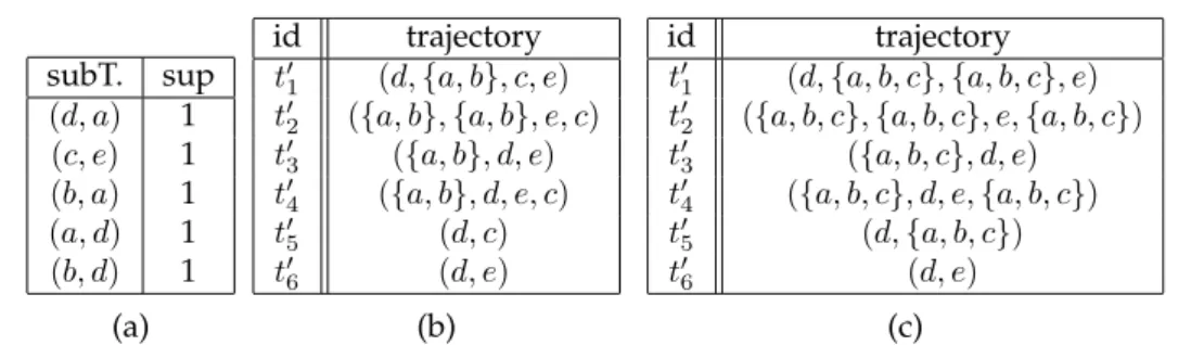
The following is an example of SEQANONin operation.
Example 4. We will demonstrate the operation of SEQANONusing datasetT of Figure1a and
k =m = 2. The intermediate steps are illustrated in Figure4. The first iteration of the for loop
(Steps2 – 8) considers the subtrajectories of sizei = 1. It is not hard to verify that all size 1
locations have support greater (or equal) thank= 2, thus the algorithm proceeds toi= 2. For this
case, Step3computes the set of subtrajectoriesS (illustrated in Figure4a). SEQANONconsiders
subtrajectorys = (d, a), which is the first subtrajectory inS. Then, the algorithm setsl1 = a,
becauseais the location with the lowest support in(d, a)(Step6), andl2 = b, becaused(a, b)is
minimum, according to Figure1b (Step7). Finally, in Step8SEQANONreplacesaandbwith the
generalized location{a, b}insand in all the trajectories ofT′. After these replacements, we have
s= (d,{a, b})and the resultantT′ shown in Figure4b. Since, we still havesup(s,T′)< k, the
while loop (Steps5 –8) is executed again. This time, l1 = {a, b}and l2 =c, and the algorithm
constructs the generalized datasetT′, shown in Figure4c. The remaining steps of the algorithm
SEQANONdo not changeT′. Thus, the final output of SEQANONis shown in Figure4c.
Time complexity analysis. We first compute the time needed by SEQANONto execute theforloop (Steps2–8). For each iteration of this loop, the setS is constructed, sorted, and explored. The cost of creating and sorting this set isO(|L|i)and O(|L|i ·log(|L|i)), respectively, where|L|is the size of the location set used inT andi is the loop counter. These bounds are very crude approximations, which correspond to the case in which all sizeisubtrajectories have support lower thank. In practice, however, the number of the subtrajectoriesswithsup(s,T′)< kis a small fraction ofO(|L|i), which depends heavily on the datasetT and the value of the anonymization parameterk. The cost of exploring the setS(Steps4–8) isO(|L|i·(|L|+|T′|))because, for each element ofS, the algorithm needs
to consider at mostO(|L|)locations and access all trajectories inT′. Thus, each iteration
subT. sup (d, a) 1 (c, e) 1 (b, a) 1 (a, d) 1 (b, d) 1
(a)
id trajectory
t′
1 (d,{a, b}, c, e)
t′
2 ({a, b},{a, b}, e, c)
t′
3 ({a, b}, d, e)
t′4 ({a, b}, d, e, c)
t′
5 (d, c)
t′
6 (d, e)
(b)
id trajectory
t′
1 (d,{a, b, c},{a, b, c}, e)
t′
2 ({a, b, c},{a, b, c}, e,{a, b, c})
t′
3 ({a, b, c}, d, e)
t′4 ({a, b, c}, d, e,{a, b, c})
t′
5 (d,{a, b, c})
t′
6 (d, e)
(c)
Figure 4: (a)SetSfor subtrajectories of sizei = 2and the respective supports,(b) Trans-formed datasetT′after S
EQANONhas processed the subtrajectory(d, a), and(c)The final 22-anonymous resultT′, produced by S
EQANON.
complexity of SEQANONisO
m P
i=1
(|L|i·(log(|L|i) +|L|+|T′|))).
4.2
The SD-SEQANON
algorithm
SD-SEQANONtakes as input an original trajectory datasetT, the anonymization parame-terskandm, and a location taxonomy, and returns thekm-anonymous counterpartT′ofT.
The algorithm operates similarly to SEQANON, but it takes into account both the Euclidean distance and the semantic similarity of locations, when it applies generalization to them.
The pseudocode of SD-SEQANONis provided in Algorithm SD-SEQANON. Notice that SD-SEQANONand SEQANONdiffer in Step 7. This is because SD-SEQANON calculates the product of the Euclidean distance for the locationsl1andl2, and theSDmeasure for the generalized location{l1, l2}(see Definition7). Thus, it aims at creating a generalized location, which consists of locations that are close in proximity and are semantically sim-ilar. The time complexity of SD-SEQANONis the same as that of SEQANON, because the computation in Step7does not affect the complexity.
Algorithm: SD-SEQANON
Input: A datasetT, a locations hierarchy and anonymization parameterskandm
Output: Akm
-anonymous datasetT′corresponding toT
1 T′:=T // Initialize output 2 fori:= 1tomdo
3 LetSbe the set of subtrajectoriessofT with sizeisuch thatsup(s,T′)< ksorted by
increasing support
4 foreachs∈ Sdo
5 whilesup(s,T′)< kdo
6 Find the locationl1ofswith the minimum support inT′
7 Find the locationl26=l1with the minimumd(l1, l2)· SD({l1, l2})
8 Replace all occurrences ofl1andl2inT′andswith{l1, l2}
4.3
The U-SEQANON
algorithm
The U-SEQANONalgorithm takes as input an original trajectory datasetT, anonymization parametersk,m and δ, as well as a utility constraint setU. The algorithm differs from SEQANON and SD-SEQANONalong two dimensions. First, the km-anonymous dataset it produces satisfiesU, hence it meets the data publishers’ utility requirements. Second, it additionally employs suppression (i.e., removes locations from the resultant dataset), when generalization alone is not sufficient to enforcekm-anonymity.
Algorithm: U-SEQANON
Input: A datasetT, utility constraint setU, and anonymization parametersk,m, andδ
Output: Akm
-anonymous datasetT′corresponding toT
1 T′:=T // Initialize output 2 fori:= 1tomdo
3 LetSbe the set of subtrajectoriessofT with sizeisuch thatsup(s,T′)< ksorted by
increasing support
4 foreachs∈ Sdo
5 whilesup(s,T′)>0orsup(s,T′)< kdo
6 Find the locationl1ofswith the minimum support inT′
7 Find the utility constraintu∈ Uthat contains the locationl1
8 Find the locationl26=l1, l2∈uwith the minimumd(l1, l2)
9 ifCannot find locationl2then
10 Suppress locationl1fromT′
11 ifMore thanδ%of locations have been suppressedthen 12 Exit:Uis not satisfied
13 else
14 Replace all occurrences ofl1andl2inT′andswith{l1, l2}
15 returnT′
The pseudocode of U-SEQANONis provided in Algorithm U-SEQANON. As can be seen, the algorithm initializesT′ (Step1) and then follows the apriori principle (Steps2 –14).
After constructing and sortingS, U-SEQANONiterates over each subtrajectory inS and applies generalization and/or suppression, until its support is either at leastkor0(Steps 3–5). Notice thatsup(s,T′) = 0corresponds to an empty subtrajectorys(i.e., the result of
suppressing all locations ins), which does not require protection. Next, U-SEQANONfinds the locationl1with the minimum support inT′and the utility constraint that contains it (Steps6–7). Then, the algorithm finds a different locationl2, which also belongs touand is as close tol1 as possible, according to the Euclidean distance (Step8). In case such a location cannot be found (i.e., when there is a single generalized location that contains all locations inu), U-SEQANONsuppressesl2fromT′(Steps9–10). If more thanδ%of loca-tions have been suppressed,Ucannot be satisfied and the algorithm terminates (Steps11– 12). Otherwise, U-SEQANONgeneralizesl1andl2together and replaces every occurrence of either of these locations with the generalized location{l1, l2}(Step14). The algorithm repeats Steps2–14as long as the size of the considered subtrajectories does not exceedm. After considering the subtrajectories of sizem, U-SEQANON returns thekm-anonymous datasetT′that satisfiesU, in Step15.
The following is an example of U-SEQANONin operation.
# U C
1 {b, c}
2 {a, d, e}
(a)
id trajectory
t′
1 ({a, d},{a, d}, c, e)
t′
2 (b,{a, d}, e, c)
t′
3 ({a, d},{a, d}, e)
t′4 (b,{a, d}, e, c)
t′
5 ({a, d}, c)
t′
6 ({a, d}, e) (b)
id trajectory
t′
1 ({a, d, e},{a, d, e},{b, c},{a, d, e})
t′
2 ({b, c},{a, d, e},{a, d, e},{b, c})
t′
3 ({a, d, e},{a, d, e},{a, d, e})
t′4 ({b, c},{a, d, e},{a, d, e},{b, c})
t′
5 ({a, d, e},{b, c})
t′
6 ({a, d, e},{a, d, e})
(c)
Figure 5: (a)Set of Utility Constraints (b)Transformed datasetT′ after the processing of
subtrajectory(d, a), and(c)The final22-anonymous resultT′meeting the provided set of U C
T, shown in Figure1a, the utility constraint set in Figure5a,k =m= 2, andδ= 5%. During
the first iteration of the for loop (Steps2–14),U-SEQANONconsiders the subtrajectories of size
i= 1, which all have a support of at least2. Thus, the algorithm considers subtrajectories of size
i= 2, and constructs the setSshown in Figure4a (Steps4–3). Then,U-SEQANONconsiders
the subtrajectorys = (d, a)in S, which has the lowest support inT′ (Step6). Next, in Steps6
–8, the algorithm finds the locationl1 =a, which has the lowest support inT′, and the location
l2=d, which belongs to the same utility constraint asaand is the closest to it – see also the map in
Figure1b. After that, the algorithm replacesaanddwith the generalized location{a, d}insand
all the trajectories ofT′ (Step14). After these replacements,s= ({a, d},{a, d})and the trajectory
datasetT′ is as shown in Figure4b. Since the support ofsin T′ is at leastk, the while loop in
Step5 terminates and the algorithm checks the next problematic subtrajectory,s = (c, e). After
considering all problematic subtrajectories of size 2, U-SEQANON produces the 22-anonymous
dataset in Figure5c, which satisfiesU.
The time complexity of U-SEQANONis the same as that of SEQANON, in the worst case whenUis comprised of a single utility constraint that contains all locations inL,Scontains
O(|L|i)subtrajectories with support in(0, k), andδ= 100. Note that the cost of suppressing a locationl1 isO(|T′|)(i.e., the same as that of replacing the locationsl1and l2 with the generalized location(l1, l2)in all trajectories inT′).
5
Experimental evaluation
In this section, we provide a thorough experimental evaluation of our approach, in terms of data utility and efficiency.
In addition, we used a dataset that has been derived from the Gowalla location-based social networking website and contains the check-ins (locations) of users between February 2009 and October 2010 [10]. In our experiments, we used aggregate locations of86,061users, in the state of New York and nearby areas. This dataset is referred to as Gowalla and contains 86,061trajectories, whose average length is3.92, and662locations.
To study the effectiveness of our approach, we compare it against the NGRAMSmethod [7], discussed in Section2, using the implementation provided by the authors of [7]. Con-trary to [5], the NGRAMSmethod was developed for count query answering. Thus, a com-parison between the NGRAMSmethod and ours allows us to evaluate the effectiveness of our approach with respect to count query answering. For this comparison, we set the pa-rameterslmax,nmax, andeto the values20,5, and0.1, respectively, which were suggested in [7]. Unless otherwise stated, k is set to5 andm is set to2. The location taxonomies were created as in [35]. Specifically, each non-leaf node in the taxonomy for the Oldenburg (respectively, Gowalla) dataset has5(respectively,6) descendants.
Measures. To measure data utility we used theAverage Relative Error (ARE)measure [21], which has become a defacto data utility indicator [24,31]. ARE estimates the average num-ber of trajectories that are retrieved incorrectly, as part of the answers to a workload of COUNT queries. Low ARE scores imply that anonymized data can be used to accurately estimate the number of co-occurrences of locations. We used workloads of 100 COUNT queries, involving randomly selected subtrajectories with size in[1,2], because the output of the NGRAMSmethod contained very few longer trajectories (see Figure10b).
In addition, we usedKullback–Leibler divergence(KL-divergence), an information-theoretic measure that quantifies information loss and is used widely in the anonymization literature [16,19]. In our context, KL-divergence measures support estimation accuracy based on the difference between the distribution of the support of a set of subtrajectoriesS, in the original and in the anonymized data2. LetPS (respectively,QS) be the distribution of the support of the subtrajectories inS in the datasetT (respectively, generalized datasetT′).
TheKL-divergence betweenPSandQSis defined as:
DKL(PS kQS) =
X
s∈S
PSln
P S
QS
Clearly, low values inKL-divergence are preferred, as they imply that a small amount of information loss was incurred to generalize the subtrajectories inS. Furthermore, we used statistics on the number, size, and distance, for the locations in generalized data.
To evaluate the extent to which SD-SEQANONgeneralizes semantically close locations together, we compute asemantic similarity penaltyPfor the generalized dataset, as follows:
P(T′) = X
t′∈T′ 1
|t′|· X
l′∈t′
SD(l′) !
|T′|
wheret′is a trajectory in the generalized datasetT′, with size|t′|, and|T′|is the number of
trajectories inT′. P reflects how semantically dissimilar are (on average) the locations in
the trajectories in the generalized dataset. The values inP(T′)are in[0,1]and lower values
imply that the generalized locations inT′contain more semantically similar locations.
To evaluate the ability of the SEQANONand NGRAMS algorithms to permit sequential pattern mining, we employ a testing framework similar to that of Gionis et al. [17]. In more detail, we construct random projections of the datasets produced by our algorithms, by replacing every generalized location in it with a random location, selected from that generalized location. Then, we use Prefixspan [30], to obtain the frequent sequential pat-terns (i.e., the sequential patpat-terns having support larger than a threshold) in the original, the output of NGRAMS and the projected datasets. Next, we calculate the percentage of the frequent sequential patterns of the original dataset that are preserved in the output of NGRAMS and in the projected datasets. We also calculate the percentage of the frequent sequential patterns in the output of NGRAMSand in the projected datasets that are not fre-quent in the original dataset. Clearly, an anonymized dataset (produced by either NGRAMS or by our algorithms) allows accurate mining, when: (i)a high percentage of its frequent sequential patterns are frequent in the original dataset, and(ii)a low percentage of its fre-quent sefre-quential are not frefre-quent in the original dataset.
5.1
Data utility
In this section, we evaluate the effectiveness of the SEQANON, SD-SEQANON, and U-SEQANONalgorithms at preserving data utility.
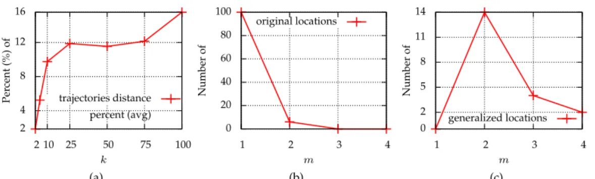
SEQANON. We begin by evaluating the data utility offered by the SEQANONalgorithm, using some general statistics, computed for the output of this algorithm on the Oldenburg dataset. Specifically, we measured the number of the locations that were released intact (referred to as original locations) and the number of the locations that were generalized. For the generalized locations, we also measured their average size and distance. Initially, we varied the anonymization parameterkin [2, 100]. Our results are summarized in Fig-ures6a-7a.
In Figure6a, we present the number of the original locations, as a function ofk. As ex-pected, increasingkled to fewer original locations. In Figure6b, we report the number of generalized locations. Whenkincreases, more locations are grouped together to ensure
km-anonymity, leading to fewer generalized locations. As an immediate result, the average number of locations in a generalized location increased, as shown in Figure6c. In addition, we report the average Euclidean distance of all locations contained in each generalized lo-cation. We normalize this distance as a percentage of the maximum possible distance (i.e., the distance between the two furthermost points). This percentage quantifies the distortion
2 5 8 11
2 10 25 50 75 100
Number
of
k
original locations
(a)
6 9 13 16 19
2 10 25 50 75 100
k
generalized locations
(b)
5 8 11 14 16
2 10 25 50 75 100
k
locations per generalized location (avg)
(c)
in a generalized location. In Figure7a, we illustrate the distance percentage as a function of
k. Whenkincreases, more locations are grouped together in the same generalized location, leading to more distortion. As SEQANONfocuses on minimizing the Euclidean distance of locations in each generalized location, the distortion is relatively low and increases slowly. To show the impact ofmon data utility, we setk = 5and variedmin [1,4]. Since our dataset has an average of 4.72 locations per trajectory,m= 3(respectively,m= 4) means that the adversary knows approximately65%(respectively,85%) of a user’s locations. So, form = 3andm = 4, we expect significant information loss. On the contrary, for m = 1, all locations have support greater thank = 5, so no generalization is performed and no generalized locations are created. Asmincreases, more generalizations are performed in order to eliminate subtrajectories with low support. This leads to fewer generalized locations with larger sizes. These results are shown in Figures7b-8b.
Also, we evaluated the impact of dataset size on data utility, using various random subsets of the original dataset, containing2,000,5,000,10,000, and15,000records. In Figure8c, we illustrate the number of original locations for variable dataset sizes. For larger datasets, this number increases, as the support of single locations is higher. Consequently, the sup-port of subtrajectories increases, and fewer locations are generalized. This leads to more generalized locations, with lower average size, and lower distance, as can be seen in Fig-ures9a-9c. 2 4 8 12 16
2 10 25 50 75 100
Per cent (%) of k trajectories distance percent (avg) (a) 0 20 40 60 80 100
1 2 3 4
Number of m original locations (b) 0 2 5 8 11 14
1 2 3 4
Number
of
m
generalized locations
(c)
Figure 7: number of(a)average percent of distance in generalized locations, (b)original (non generalized) locations published and(c)generalized locations published
0 10 20 30 40 50
1 2 3 4
Number of m locations per generalized location (avg) (a) 0 10 20 30 40
1 2 3 4
Per cent (%) of m trajectories distance percent (avg) (b) 2 3 4 5 6
2 5 10 15 18
Number
of
|T |(·103
)
original locations
(c)
7 9 12 14
2 5 10 15 18
Number
of
|T |(·103
)
generalized locations
(a)
6 8 10 12 14
2 5 10 15 18
Number
of
|T |(·103
)
locations per generalized location (avg)
(b)
5 6 7 8
2 5 10 15 18
Per
cent
(%)
of
|T |(·103
)
trajectories distance percent (avg)
(c)
Figure 9: (a)number of generalized locations published,(b)average generalized location size and(c)average percent of distances in generalized locations
SEQANONvs. NGRAMS.In this section, we report the count of the subtrajectories of
dif-ferent sizes that are created by the NGRAMSmethod. In addition, we report the ARE and
KL-divergence scores for the SEQANONand NGRAMSmethods. Finally, we report the per-centage of the frequent sequential patterns of the original dataset that are preserved in the anonymous dataset and the percentage of frequent sequential patterns of the anonymous dataset that are not frequent on the original dataset. The results of comparing NGRAMSto SD-SEQANONand to U-SEQANONwere quantitatively similar (omitted for brevity).
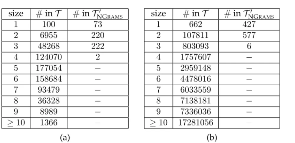
Fig. 10a reports the number of subtrajectories of different sizes that are contained in the Oldenburg dataset, denoted withT, and the output of NGRAMS, denoted withTS′EQANON. As can be seen, the output of NGRAMScontains noisy versions of only a small percent-age (0.29%) of short subtrajectories. Thus, the information of the subtrajectories of length greater than4, which correspond to72.62%of the subtrajectories in the dataset, is lost. The results of the same experiment on the Gowalla dataset, reported in Fig. 10b, are quantita-tively similar. That is, NGRAMScreated noisy versions of0.11%of the subtrajectories with 3or fewer locations, and the information of all longer subtrajectories, which correspond to 98.1%of the subtrajectories in the dataset, is lost. On the other hand, SEQANONemploys generalization, which preserves the information of all subtrajectories, although in a more aggregate form.
size #inT #inT′ NGRAMS
1 100 73
2 6955 220
3 48268 222
4 124070 2
5 177054 −
6 158684 −
7 93479 −
8 36328 −
9 8989 −
≥10 1366 −
(a)
size #inT #inT′ NGRAMS
1 662 427
2 107811 577
3 803093 6
4 1757607 −
5 2959148 −
6 4478016 −
7 6033559 −
8 7138181 −
9 7336036 −
≥10 17281056 −
(b)
Figure 10: Number of distinct subtrajectories of different sizes, for(a)the Oldenburg, and
(b)the Gowalla dataset.
are reported in Figures11c and11d.
The results with respect to KL-divergence, as a function ofm, are shown in Figure14. Specifically, Figure14a reports the result for the setSof all subtrajectories with size1(i.e., all locations) in the Oldenburg dataset, and fork= 5. As can be seen, the information loss for SEQANONwas significantly lower than that of NGRAMS, particularly for smaller val-ues ofm. Increasingmled to fewer, larger generalized locations. Thus, theKL-divergence scores of SEQANONincrease withm, while those of NGRAMSare not affected bym, for the reason explained before. Figure14b (respectively, Figure14c) reports theKL-divergence scores for100randomly selected locations (respectively, subtrajectories with size2) in the Gowalla dataset. As noted previously, we did not consider longer subtrajectories, as all but 6of the subtrajectories in the output of NGRAMShave size at most2. Again, SEQANON out-performed NGRAMSby a large margin, which demonstrates that our method can preserve the distribution of the support of subtrajectories better. Specifically, theKL-divergence scores for our method were at least20%and up to4.3times lower (better) than those for NGRAMS. Similar results were obtained for largerkvalues (omitted for brevity).
Next, we present the results of experiments, in which we evaluated the ability of the algo-rithms to support frequent sequential pattern mining. Specifically, we report the percentage of the frequent sequential patterns of the original dataset that are preserved in the anony-mous dataset and the percentage of frequent sequential patterns of the anonyanony-mous dataset that are not frequent on the original dataset. In order to get a more accurate statistical dis-tribution we used2000randomly projected anonymous datasets3. In our experiments, we mined the Oldenburg and Gowalla dataset, using a support threshold of0.83%and0.14%, respectively.
Figures12aand12bpresent the median and standard deviation of the percentage of fre-quent sefre-quential patterns that were preserved in the anonymous dataset, when SEQANON was applied with akin[2,100]and NGRAMSwith the default parameters, on Oldenburg and Gowalla datasets respectively. The results for SEQANONare significantly better than those of NGRAMS. Specifically, SEQANONreported at least48%and up to192%more fre-quent patterns than NGRAMS. Note also that SEQANONperforms better whenkis smaller, because it applies a lower amount of generalization.
1.34 4 6 8 10
2 10 25 50 75 100
ARE
k
NGRAMS
SEQANON
(a)
0 1 2 4 6 8 10 12
1 2 3 4
m
NGRAMS
SEQANON
(b)
1.4 5 10 15.5
2 10 25 50 75 100
ARE
k
NGRAMS
SEQANON
(c)
0.8 5 10 15 20 25
2 10 25 50 75 100
k
NGRAMS
SEQANON
(d)
Figure 11: ARE for queries involving100randomly selected subtrajectories(a)with size in [1,2], in the Oldenburg dataset (varyingk),(b)with size in[1,2], in the Oldenburg dataset (varyingm),(c)with size1, in the Gowalla dataset (varyingk), and(d)with size2in the Gowalla dataset (varyingk).
Figures12cand 12dreport the median and standard deviation of the percentage of fre-quent sefre-quential patterns of the anonymous dataset that are not frefre-quent on the original dataset, when SEQANONwas applied with a kin[2,100]and NGRAMS with the default parameters, on Oldenburg and Gowalla datasets respectively. Again, the results for SE -QANONare better than those of NGRAMS. In more detail, the percentage of patterns that are not frequent in the original dataset but are frequent in the anonymized dataset was up to1.2times lower (on average45%lower) for SEQANONcompared to NGRAMS. Note that askincreases, the percentage of such patterns for SEQANONdecreases, because fewer patterns are frequent in the anonymized dataset.
Figures13a and 13breport the percentage of frequent sequential patterns preserved in anonymous dataset and the percentage of frequent sequential patterns of the anonymous dataset that are not frequent on the original dataset. We setk = 5and varymin[1,4]for SEQANON, while NGRAMS was executed with the default parameters. Larger values of
mresult in more generalization. Thus, SEQANONpreserves at least20%and up to650% more frequent patterns frequent than NGRAMS, while the percentage of patterns that are incorrectly identified as frequent is lower by at least50%and up to500%compared to that for NGRAMS. The corresponding results for Gowalla were qualitatively similar (omitted for brevity).
ap-13 20 25 30 35 38
2 10 25 50 75 100
%
k
NGRAMS
SEQANON
(a)
40 50 60 70
2 10 25 50 75 100
%
k
NGRAMS
SEQANON
(b)
10 15 20 25 30
2 10 25 50 75 100
%
k
NGRAMS
SEQANON
(c)
5.8 6 6.3 6.6
2 10 25 50 75 100
%
k
NGRAMS
SEQANON
(d)
Figure 12: Percentage of frequent sequential patterns preserved in anonymous dataset (me-dian) for varyingkon(a)Oldenburg dataset, (b)Gowalla dataset, and percentage of fre-quent sefre-quential patterns of the anonymous dataset that are not frefre-quent on the original (median) for varyingkon(c)Oldenburg dataset and(d)Gowalla dataset.
13 20 40 60 80 100
1 2 3 4
%
m
NGRAMS
SEQANON
(a)
0 5 10 15 20 25 30
1 2 3 4
%
m
NGRAMS
SEQANON
(b)
Figure 13:(a)Percentage of frequent sequential patterns preserved in anonymous dataset (median) and(b)percentage of frequent sequential patterns of the anonymous dataset that are not frequent on the original (median) on Oldenburg dataset for varyingm.
plications that require preserving data truthfulness.
SD-SEQANON. In this section, we evaluate the data utility offered by SD-SEQANON, us-ing statistics computed for the output of this algorithm. Figure15a (respectively,15b) re-ports the average distance of all locations that are mapped to each generalized location, as a function of k, for the Oldenburg (respectively, the Gowalla) dataset. Increasing k
SD-0 100 200 300 400 500
1 2 3 4
K L -diver gence m NGRAMS
SEQANON
(a) 0 200 400 600 850
1 2 3 4
m
NGRAMS
SEQANON
(b) 0 2 4 6 8
1 2 3 4
m
NGRAMS
SEQANON
(c)
Figure 14:KL-divergence for the distribution of the support of(a)all locations in the Old-enburg dataset, (b) 100 randomly selected locations in the Gowalla dataset, and (c)100 randomly selected subtrajectories of size2in the Gowalla dataset.
9.8 12 14 16 18 20.3
2 10 25 50 75 100
%
k
SEQANON
SD-SEQANON
(a) 9 20 30 40 53
2 10 25 50 75 100
k
SEQANON
SD-SEQANON
(b)
Figure 15: Average percent of distance in generalized locations for(a)Oldenburg and(b)
Gowalla dataset. 0.08 0.2 0.4 0.6 0.8 1
2 10 25 50 75 100
P
k
SEQANON
SD-SEQANON
(a)
0.13 0.3 0.45 0.65
2 10 25 50 75 100
k
SEQANON
SD-SEQANON
(b)
Figure 16: Semantic similarity penaltyP(T′)for(a)Oldenburg and(b)Gowalla dataset.
SEQANONtakes into account not only the distance but also the semantic similarity of lo-cations, when performing generalization. Thus, as can be seen in Figures16a and 16b, the SD-SEQANONalgorithm performs much better than SEQANONwith respect to the
better than those for SEQANON). This demonstrates that SD-SEQANONgeneralizes more semantically close locations together.
Figure17presents the average size of generalized locations, the average percent of dis-tance in generalized locations, and the semantic similarity penaltyP, as a function ofm. In these experimentskwas set to50. As can be seen, increasingmleads the algorithms to construct fewer, larger generalized locations, which are comprised of more distant and less semantically close locations. As expected, SEQANONgeneralized together locations that are closer in proximity (see Figure17b) but more semantically distant (see Figure17c).
2 50 100 150 200 250 300 331
1 2 3 4
#
m
SEQANON
SD-SEQANON
(a)
0 3 6 9 12
1 2 3 4
%
m
SEQANON
SD-SEQANON
(b)
1.8 15 30 45 60 75 87
1 2 3 4
%
m
SEQANON
SD-SEQANON
(c)
Figure 17: (a)average generalized location size, (b)average percent of distance in gener-alized locations and(c)average percent of similarity in generalized locations for k = 50 (Gowalla dataset).
U-SEQANON.This section reports results for the U-SEQANONalgorithm, which was con-figured with three different utility constraint sets, namelyU1,U2andU3, and a suppression thresholdδ = 10. The utility constraints in each of these sets contain a certain number of semantically close locations (i.e., sibling nodes in the location taxonomy), as shown in Fig-ure18. Note thatU3is more difficult to satisfy thanU1, as the number of allowable ways to generalize locations is smaller.
U1 U2 U3
|u1|= 50 |u1|= 25 |u1|= 20
|u2|= 50 |u2|= 25 |u2|= 14
|u3|= 25 |u3|= 16
|u4|= 25 |u4|= 14
|u5|= 18
|u6|= 18


![Figure 11: ARE for queries involving 100 randomly selected subtrajectories (a) with size in [1, 2], in the Oldenburg dataset (varying k), (b) with size in [1, 2], in the Oldenburg dataset (varying m), (c) with size 1, in the Gowalla dataset (varying k), an](https://thumb-eu.123doks.com/thumbv2/123dok_br/18199261.333281/22.892.148.643.131.548/figure-involving-randomly-selected-subtrajectories-oldenburg-oldenburg-gowalla.webp)
