The Objectivity Measurement of
Frequent Patterns
Phi-Khu Nguyen, Thanh-Trung Nguyen
Abstract—Frequent pattern mining is a basic problem in data mining and knowledge discovery. The discovered patterns can be used as the input for analyzing association rules, mining sequential patterns, recognizing clusters, and so on.
However, there is a posed question that how is objectivity measurement of frequent patterns? Specifically, in market basket analysis problem to find out association rules, whether or not the frequent patterns discovered represent exactly the needs of all customers. Or, these frequent patterns were only created by a few customers with too many purchases.
In this paper, a mathematical space will be introduced with some new related concepts and propositions to design a new algorithm answering the above questions.
Index Terms—association rule, data mining, frequent patterns mining, objectivity measurement.
I. SPACE OF BOOLEAN CHAINS
Let B = {0,1}, Bm is the space of m-tuple Boolean chains, whose elements are s = (s1, s2, .. , sm), si∈ B, i = 1,..,m.
A. Definitions
A Boolean chain a = (a1, a2, .. , am) is said to cover another
Boolean chain b = (b1, b2, .. , bm) – or b is covered by a, if for
each i ∈ {1,..,m} the condition bi = 1 implies that ai = 1. For
instance, (1,1,1,0) covers (0,1,1,0).
Let S be a set of n Boolean chains. If there are k chains in S covering a chain u = (u1, u2, .. , um) then u is called a form with
a frequency of k in S and [u; k] is called a pattern of S. For instance, if S = { (1,1,1,0), (0,1,1,1), (0,1,1,0), (0,0,1,0), (0,1,0,1) } then u = (0,1,1,0) is a form with a frequency 2 in S and [(0,1,1,0); 2] is a pattern of S.
A pattern [u; k] of S is called a maximal pattern if and only if the frequency k is the maximal number of Boolean chains in S. In the above instance, [(0,1,1,0); 3] is a maximal pattern in S.
The set P of all maximal patterns in S whose forms are not covered by any form of other maximal pattern, is called a representative set and each element of P is called a representative pattern of S.
Based on this definition, the following proposition is trivial:
Proposition 1: Let S be a set of m-tuple Boolean chains and
P be the representative set of S, then any couple of two elements in P are not coincided.
Manuscript received June 30, 2010.
Phi-Khu Nguyen is with University of Information Technology, Vietnam National University HCM City, Vietnam (e-mail: [email protected]).
Thanh-Trung Nguyen is with the Department of Computer Science, University of Information Technology, Vietnam National University HCM City, Vietnam (e-mail: [email protected]).
By listing all of n elements of the set S of m-tuple Boolean chains in a Boolean n×m matrix, each element [u; k] of the representative set forms a maximal rectangle with maximal height of k in S set.
For instance, if S = { (1,1,1,0), (0,1,1,1), (1,1,1,0), (0,1,1,1), (0,0,1,1) }, then representative set of S consists of five representative patterns: P = { [(1,1,1,0); 2], [(0,1,1,0); 4], [(0,0,1,0); 5], [(0,1,1,1); 2], [(0,0,1,1); 3] }. All of five elements of S are listed in a form of Boolean 5×4 matrix, as follows:
A 5x4 matrix: and [(0,1,1,0); 4]:
1 1 1 0 1
1 1
00 1 1 1 0 1 1 1
1 1 1 0 1
1 1
00 1 1 1 0
1 1
10 0 1 1 0 0 1 1
Fig. 1. A 5x4 matrix for [(0,1,1,0); 4].
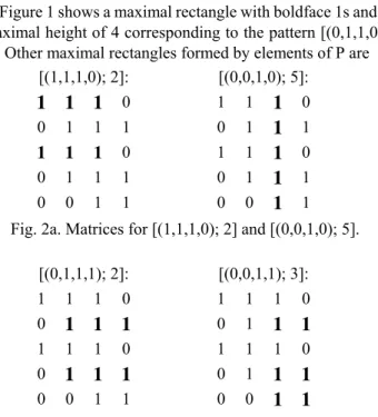
Figure 1 shows a maximal rectangle with boldface 1s and a maximal height of 4 corresponding to the pattern [(0,1,1,0); 4]. Other maximal rectangles formed by elements of P are
[(1,1,1,0); 2]: [(0,0,1,0); 5]:
1
1
1
0 1 11
00 1 1 1 0 1
1
11 1 1 0 1 1
1
00 1 1 1 0 1
1
10 0 1 1 0 0 1 1
Fig. 2a. Matrices for [(1,1,1,0); 2] and [(0,0,1,0); 5]. [(0,1,1,1); 2]: [(0,0,1,1); 3]:
1 1 1 0 1 1 1 0
0
1
1
1
0 11 1
1 1 1 0 1 1 1 0
0
1
1
1
0 11 1
0 0 1 1 0 0 1 1
B. Binary Relations
Let a = (a1, a2, .. , am) and b = (b1, b2, .. , bm) be two m-tuple
Boolean chains, then a = b if and only if ai = bi for any i =
1,..,m. Otherwise, it is denoted by a ≠ b.
Given patterns [u; p] and [v; q] in S, [u; p] is contained in [v; q] – denoted by [u; p] ⊆ [v; q], if and only if u = v and p ≤ q. To negate, the operator ! is used e.g. [u; p] !⊆ [v; q]
The minimum chain of a, b – denoted by a ∩ b, is a chain z = (z1, z2, .. , zm) determined by z = a ∩ b where zk = min(ak,
bk) with k = 1,..,m.
The minimum pattern of [u; p] and [v; q] is a pattern [w; r], denoted by [u; p] ∩ [v; q], defined as follows: [u; p] ∩ [v; q] = [w; r] here w = u ∩ v and r = p + q.
II. AN IMPROVED ALGORITHM A. Theorem 1: for Adding a New Element
Given S be a set of m-tuple Boolean chains and P representative set of S. For [u; p], [v; q]∈ P and z ∉ S, let [u; p] ∩ [z; 1] = [t; p+1], [v; q] ∩ [z; 1] = [d; q+1]. Only one of the following cases must be satisfied:
i. [u; p] ⊆ [t; p+1] and [u; p] ⊆ [d; q+1], t = d ii. [u; p] ⊆ [t; p+1] and [u; p] !⊆ [d; q+1], t ≠ d iii. [u; p] !⊆ [t; p+1] and [u; p] !⊆ [d; q+1].
Proof: From Proposition 1, obviously u ≠ v. The theorem is proved if the following claim is true: Let
(a): u = t , u = d , and t = d; (b): u = t , u ≠ d , and t ≠ d; (c): u ≠ t and u ≠ d,
only one of the above statements is correct.
By the method of induction on the number m of entries of chain, in the first step, we show that the claim is correct if u and v differ at only one kth entry.
Without loss of generality, we assume that uk = 0 and vk =
1. The following cases must be true:
- Case 1: zk = 0; Then min(uk, zk) = min(vk, zk) = 0, hence
t = u ∩ z = (u1, u2, .. , 0, .. , um) ∩ (z1, z2, .. , 0, .. , zm) = (x1,
x2, .. , 0, .. , xm), xi = min(ui, zi), for i = 1,..,m, i≠k;
d = v ∩ z = (v1, v2, .. , 1, .. , vm) ∩ (z1, z2, .. , 0, .. , zm) = (y1,
y2, .. , 0, .. , ym), yi = min(vi, zi), for i = 1,..,m, i≠k.
From the assumption ui = vi when i ≠ k thus xi = yi, so t = d.
Hence, if u = t then u = d and (a) is correct. On the other hand, if u ≠ t then u ≠ d, therefore (c) is correct.
- Case 2: zk = 1; We have min(uk, zk) = 0, min(vk, zk) = 1
and t = u ∩ z = (u1, u2, .. , 0, .. , um) ∩ (z1, z2, .. , 1, .. , zm) = (x1,
x2, .. , 0, .. , xm), xi = min(ui, zi), for i = 1,..,m, i≠k;
d = v ∩ z = (v1, v2, .. , 1, .. , vm) ∩ (z1, z2, .. , 1, .. , zm) = (y1,
y2, .. , 1, .. , ym), yi = min(vi, zi), for i = 1,..,m, i≠k.
So, t ≠ d. If u = t then u ≠ d, thus the statement (b) is correct.
In summary, the above claim is true for any u and v of S that differ only at one entry.
By induction in the second step, it is assumed that the claim is true if u and v differ at r entries, and only one of the three statements (a), (b) or (c) is true.
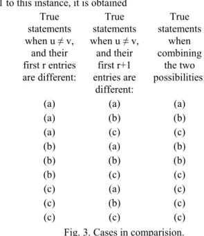
Without loss of generality, we assume that the first r entries of u and v are different, and they differ at (r+1)-th entries. Applying the same method in the first step where r =
1 to this instance, it is obtained True
statements when u ≠ v,
and their first r entries are different:
True statements when u ≠ v,
and their first r+1 entries are
different:
True statements
when combining
the two possibilities: (a) (a) (a) (a) (b) (b) (a) (c) (c) (b) (a) (b) (b) (b) (b) (b) (c) (c) (c) (a) (c) (c) (b) (c) (c) (c) (c)
Fig. 3. Cases in comparision.
Therefore, if u and v are different at r+1 entries, only one of the (a), (b), (c) statements is correct. The above claim is true, and Theorem 1 is proved.
B. Algorithm: for Finding a New Representative Set Let S be a set that consists of n m-tuple Boolean chains, and P the representative set of S. If a m-tuple Boolean chain z is added to S, the following algorithm is used to determine the new representative set of S ∪ {z}:
ALGORITHM NewRepresentative( P , z )
// Finding new representative set for S when one chain is added to S.
// Input: P is a representative set of S, z: a chain added to S. // Output: The new representative set P of S ∪ {z}. 1. M = ∅ // M: set of new elements of P
2. flag1 = 0 3. flag2 = 0
4. for each x ∈ P do 5. q = x ∩ [z; 1]
6. if q ≠ 0 // q is not one chain with all elements 0 7. if x ⊆ q then P = P \ {x}
8. if [z; 1] ⊆ q then flag1 = 1 9. for each y ∈ M do 10. if y ⊆ q then 11. M = M \ {y} 12. break for 13. endif 14. if q ⊆ y then 15. flag2 = 1 16. break for 17. endif 18. endfor 19. else 20. flag2 = 1 21. endif
22. if flag2 = 0 then M = M ∪{q} 23. flag2 = 0
24. endfor
25. if flag1 = 0 then P = P ∪{ [z; 1] } 26. P = P ∪ M
C. Theorem 2: for Finding Representative Sets
Let S be a set of n m-tuple Boolean chains. The representative set of S is determined by applying NewRepresentative algorithm to each of n elements of S in turn.
Proof: This theorem is proved by induction on the number n of elements of S.
Firstly, when applying the above algorithm to the set S of only one element, this element is added into P and then P with that only element is the representative set of S. Thus, Theorem 2 is proved in the case of n = 1.
Next, assume that S consists of n elements, the above algorithm is applied to S, and it is obtained a representative set P0 of p patterns. Each element of P0 allows to form a
maximal rectangle from S. When adding a new m-tuple Boolean chain z to S, it is necessary to prove that the algorithm allows to find a new representative set P of S ∪ {z}.
Indeed, with z, some new rectangle forms will be formed along with the existing rectangle forms. But some of these new rectangle forms which are covered by other rectangle forms, the so-called ‘redundant’ rectangles, need to be removed to gain P.
The fifth statement in the NewRepresentative algorithm shows that the operator ∩ is applied to z and p elements of P0
to produce p new elements belonging to P. This means z ‘scans’ all elements in the set P0 to find out new rectangle
forms when adding z into S. Consequently, three groups of 2p+1 elements in total are created from the sets P0, P, and z.
To remove redundant rectangles, we have to check whether each element of P0 is contained by elements of P or
not, and elements of P contain other one, in which z is an element in P.
Let x be an element of P0 and consider the form x ∩ z,
there are two instances: if the form of z covers the one of x then x is a new form; or if the form of x covers the one of z then z is a new form. Anyway, the frequency of the new form is always one unit greater than frequency of the original.
According to Theorem 1, with x ∈ P0, if some pattern w
contains x then w must be a new element which belongs to P, and that new element is q = x ∩ [z; 1]. To check whether x is contained by elements belonging to P, we do that whether x is contained by q or not. If x contained by q, it must be removed from the representative (line 7).
In summary, first the algorithm checks whether elements belonging to P0 is contained by elements belonging to P.
Then, the algorithm checks whether elements of P contain one other (from line 9 to line 18), and whether [z; 1] is contained by elements belonging to P or not (line 8).
Finally, the above NewRepresentative algorithm can be used to find new representative set when adding new elements to S.
III. THE OBJECTIVITY MEASUREMENT A. Association Rule Discovery
Advanced technologies have enabled us to collect large amounts of data on a continuous or periodic basis in many
fields. On one hand, these data present the potential for us to discover useful information and knowledge that we could not find before. On the other hand, we are limited in our ability to manually process large amounts of data to discover useful information and knowledge. This limitation demands automatic tools for data mining to mine useful information and knowledge from large amounts of data. Data mining has become an active area of research and development.
Association rules – a data mining methodology that is usually used to discover frequently co-occurring data items, for example, items that are commonly purchased together by customers at grocery stores. Association rule discovery problem were introduced in 1993 by Agrawal [17]. Since then, this problem has received much attention. Today the exploitation such rules is still one of the most popular way for exploiting pattern in order to conduct knowledge discovery and data mining.
Exactly, association rule discovery is the process discovering sets of value of attribute appearing frequently in data objects. From the frequent patterns, association rules can be created in order to reflect the ability of appearing simultaneously the value of attribute in the set of objects. To bring out the meaning, an association rule of X → Y reflects the occurrence of the set X conduces to the appearance of the set Y. In other words, an association rule indicates an affinity between X (antecedent) and Y (consequent). An association rule is accompanied by frequency-based statistics that describe that relationship. The two statistics that were used initially to describe these relationships were support and confidence [17].
The apocryphal example is a chain of convenience stores that performs a analysis and discovers that disposable diapers and beer are frequently bought together [8]. This unexpected knowledge is potentially valuable as it provides insight into the purchasing behavior of both disposable diaper and beer purchasing customers for the convenience store chain. So that, we can find association rules help identify trends in sales, customer psychology, etc. to make strategic layout item, business, marketing, and so on.
In short, the association rule discovery can be divided into two parts:
• Finding all frequent patterns that satisfy min-support.
• Finding all association rules that satisfy minimum confidence.
Most research in the area of association rule discovery has focused on the sub-problem of efficient frequent pattern discovery (for example, Han, Pei, & Yin, 2000; Park, Chen, & Yu, 1995; Pei, Han, Lu, Nishio, Tang, & Yang, 2001; Savasere, Omiecinski, & Navathe, 1995). When seeking all associations that satisfy constraints on support and confidence, once frequent patterns have been identified, generating the association rules is trivial.
B. The Methods of Finding Frequent Patterns
• Candidate Generation Methods: for instance, Apriori method proposed by Agrawal in piece of research [17]–[8], and algorithms rely on Apriori such as AprioriTID, Apriori-Hybrid, DIC, DHP, PHP,... in [3]–[4]–[8].
Zaki’s method relies on IT-tree and intersection part of Tidsets in order to reckon support, [3]; or J. Han’s one relies on FP-tree in order to exploit frequent patterns, [9]–[5]; or methods Lcm, DCI, ... presented in [9].
• Paralleled Methods: instances in [15]–[16]–[11]. C. Issues Need to be Solved
• Working with the varying database is the biggest challenge. Especially, it need not scan again the whole database whenever having need of adding a new element.
• A number of algorithms are effective, but their basis of mathematics and way of installation are complex.
• The limit of computer memory. Hence, combining how to store the data mining context most effectively with costing the memory least and how to store frequent patterns is also not a small challenge.
• Ability of dividing data into several parts for paralleled processing is also concerned.
Using the NewRepresentative algorithm is making good theabove problems.
D. Data Mining Context
Let O be a limited non-empty set of invoices, and I be a limited non-empty set of goods. Let R be a binary relation between O and I so that: for o ∈ O and i ∈ I, (o, i) ∈ R if and only if the invoice o includes the i-th goods. Then R is a subset of the product set O×I, and the trio (O, I, R) describes a data mining context.
For example, we have a context which is illustrated in Table 1, consisted of five invoices with the codes oj, j = 1,..,5
and four kinds of goods ik, k = 1,..,4. The corresponding
binary relation R is described in Table 2 which can be represented by a 5×4 Boolean matrix.
Table 1. Invoice details Invoice code Goods code
o1 i1 o1 i2 o1 i3 o2 i2 o2 i3 o2 i4 o3 i2 o3 i3 o3 i4 o4 i1 o4 i2 o4 i3 o5 i3 o5 i4 Table 2. Boolean matrix of data mining context
i1 i2 i3 i4 o1 1 1 1 0 o2 0 1 1 1 o3 0 1 1 1 o4 1 1 1 0 o5 0 0 1 1
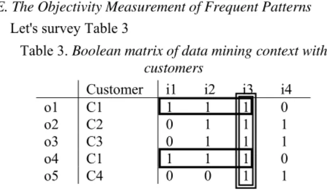
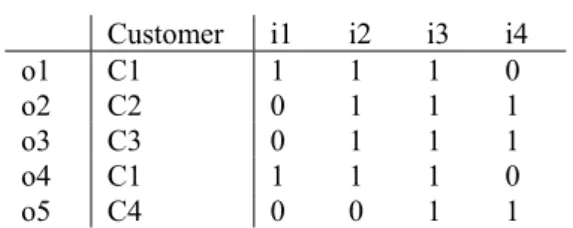
E. The Objectivity Measurement of Frequent Patterns Let's survey Table 3
Table 3. Boolean matrix of data mining context with customers
Customer i1 i2 i3 i4
o1 C1 1 1 1 0
o2 C2 0 1 1 1
o3 C3 0 1 1 1
o4 C1 1 1 1 0
o5 C4 0 0 1 1
By observing with the naked eye, we can notice immediately that the frequent pattern having form (1110) appears in two invoices (o1, o4) and is decided by the only customer C1. Meanwhile, the frequent pattern having form (0010) appears in five invoices (o1, o2, o3, o4, o5) and is decided by all four customer (C1, C2, C3, C4).
Obviously, with minsupp=40%, the both frequent patterns are satisfied. But, whether or not we can use these two frequent patterns to generate association rules, then apply these rules to prospective customers? To answer this question requires us to consider objectivity measurement of each frequent pattern. Or, more detail, we must determine the ratio of number of customers involved in the process of creating a frequent pattern to total of customers. The higher the ratio is, the better the objectivity measurement of the frequent pattern is. Viz, the frequent pattern is created by most customers. Since then, we hope that this will also correct for the majority of prospective customers.
Back to the above example, the frequent pattern (1110) has the objectivity measurement of 1/4=25%. Meanwhile, the frequent pattern (0010) has the objectivity measurement of 4/4=100%. With these parameters, business managers will have more information when making decisions.
When applying the algorithm NewRepresentative, we can solve this problem.
The tenor of the algorithm is to find out new rectangle forms created by applying the operator ∩ to corresponding line of data of current step and rectangle forms found in prior steps. However, in the first step, grouping the data mining context in order to gain the first evident rectangle forms and their corresponding height is a need. In per step, if the rectangle form created newly covers an existent rectangle form then removing the old rectangle form is necessary. Besides, it also needs to remove the newly created rectangle form if they mutually cover.
In summary, after per step, the set P whose elements differ mutually is created. This means to achieve various maximal rectangle forms in the database, as from the first line of data to the line of data corresponding to the current step.
with a minsupp of 40%.
Table 3. Boolean matrix of data mining context with customers
Customer i1 i2 i3 i4
o1 C1 1 1 1 0
o2 C2 0 1 1 1
o3 C3 0 1 1 1
o4 C1 1 1 1 0
o5 C4 0 0 1 1
Let P be the set of maximal rectangle forms of that Boolean matrix. It can be determined by following steps:
- Step 1:
Consider line 1: [(1110); 1] (l1)
Since P now is empty means should we put (l1) in P, we have:
P = { [(1110); 1; (C1-1)] } (1) - Step 2:
Consider line 2: [(0111); 1] (l2)
Let (l2) perform the ∩ operation with the elements existing in P in order to get the new elements
(l2) ∩ (1): [(0111); 1] ∩ [(1110); 1] = [(0110); 2] (n1) Considering excluded:
Considering whether or not the old elements in P is contained in the new elements:
We remain: (1)
Considering whether or not the new elements contain each other (note: (l2) is also a new element):
We remain: (l2) and (n1)
After considering excluded, it supplements the list of customers of the elements remaining:
(1): [(1110); 1; (C1-1)] (l2): [(0111); 1; (C2-1)]
(n1): [(0110); 2; (C1-1, C2-1)] //because (n1) is generated by (l2) and (1)
Putting the elements into P, we have: P = { [(1110); 1; (C1-1)] (1)
[(0110); 2; (C1-1, C2-1)] (2) [(0111); 1; (C2-1)] (3) }
- Step 3:
Consider line 3: [(0111); 1] (l3)
Let (l3) perform the ∩ operation with the elements existing in P in order to get the new elements
(l3) ∩ (1): [(0111); 1] ∩ [(1110); 1] = [(0110); 2] (n1) (l3) ∩ (2): [(0111); 1] ∩ [(0110); 2] = [(0110); 3] (n2) (l3) ∩ (3): [(0111); 1] ∩ [(0111); 1] = [(0111); 2] (n3) Considering excluded:
Considering whether or not the old elements in P is contained in the new elements:
We remove: (2) because of being contained in (n1), and (3) because of being contained in (n3)
We remain: (1)
Considering whether or not the new elements contain
each other (note: (l3) is also a new element):
We remove: (n1) because of being contained in (n2), and (l3) because of being contained in (n3)
We remain: (n2) and (n3)
After considering excluded, it supplements the list of customers of the elements remaining:
(1): [(1110); 1; (C1-1)]
(n2): [(0110); 3; (C1-1, C2-1, C3-1)] //because (n2) is generated by (l3) and (2) (n3): [(0111); 2; (C2-1, C3-1)] //because (n3) is
generated by (l3) and (3)
Putting the elements into P, we have: P = { [(1110); 1; (C1-1)] (1)
[(0110); 3; (C1-1, C2-1, C3-1)] (2) [(0111); 2; (C2-1, C3-1)] (3) }
- Step 4:
Consider line 4: [(1110); 1] (l4)
Let (l4) perform the ∩ operation with the elements existing in P in order to get the new elements
(l4) ∩ (1): [(1110); 1] ∩ [(1110); 1] = [(1110); 2] (n1) (l4) ∩ (2): [(1110); 1] ∩ [(0110); 3] = [(0110); 4] (n2) (l4) ∩ (3): [(1110); 1] ∩ [(0111); 2] = [(0110); 3] (n3) Considering excluded:
Considering whether or not the old elements in P is contained in the new elements:
We remove: (1) because of being contained in (n1), and (2) because of being contained in (n2)
We remain: (3)
Considering whether or not the new elements contain each other (note: (l4) is also a new element):
We remove: (n3) because of being contained in (n2), and (l4) because of being contained in (n1)
We remain: (n1) and (n2)
After considering excluded, it supplements the list of customers of the elements remaining:
(3): [(0111); 2; (C2-1, C3-1)]
(n1): [(1110); 2; (C1-2)] //because (n1) is generated by (l4) and (1)
(n2): [(0110); 4; (C1-2, C2-1, C3-1)] //because (n2) is generated by (l4) and (2) Putting the elements into P, we have:
P = { [(0111); 2; (C2-1, C3-1)] (1) [(1110); 2; (C1-2)] (2)
[(0110); 4; (C1-2, C2-1, C3-1)] (3) }
- Step 5:
Consider line 5: [(0011); 1] (l5)
Let (l5) perform the ∩ operation with the elements existing in P in order to get the new elements
(l5) ∩ (2): [(0011); 1] ∩ [(1110); 2] = [(0010); 3] (n2) (l5) ∩ (3): [(0011); 1] ∩ [(0110); 4] = [(0010); 5] (n3) Considering excluded:
Considering whether or not the old elements in P is contained in the new elements:
We remain: (1), (2), and (3)
Considering whether or not the new elements contain each other (note: (l5) is also a new element):
We remove: (l5) because of being contained in (n1), and (n2) because of being contained in (n3)
We remain: (n1) and (n3)
After considering excluded, it supplements the list of customers of the elements remaining:
(1): [(0111); 2; (C2-1, C3-1)] (2): [(1110); 2; (C1-2)]
(3): [(0110); 4; (C1-2, C2-1, C3-1)]
(n1): [(0011); 3; (C2-1, C3-1, C4-1)] //because (n1) is generated by (l5) and (1)
(n3): [(0010); 5; (C1-2, C2-1, C3-1, C4-1)] //because (n3) is generated by (l5) and (3) Putting the elements into P, we have:
P = { [(0111); 2; (C2-1, C3-1)] (1) [(1110); 2; (C1-2)] (2)
[(0110); 4; (C1-2, C2-1, C3-1)] (3) [(0011); 3; (C2-1, C3-1, C4-1)] (4) [(0010); 5; (C1-2, C2-1, C3-1, C4-1)] (5) }
So, the frequent patterns satisfy minsupp = 40% (2/5) is listed:
{ {i2, i3, i4} (2/5); {i1, i2, i3} (2/5); {i2, i3} (4/5);
{i3, i4} (3/5); {i5} (5/5) }
However, when considering the objective measurement or the impact measurement of customer, we clearly see that the frequent pattern {i1, i2, i3} (2/5) just was created by only customer C1. Thus, when analyzing, we will have better information about the objective measurement of this frequent pattern, viz. 1/4=25%. In addition, the objective measurement of {i2, i3, i4} (2/5) is 2/4=50%, {i2, i3} (4/5) is 3/4=75%, {i3, i4} (3/5) is 3/4=75%, and {i5} (5/5) is 4/4=100%.
IV. CONCLUSIONS AND FUTURE WORK
This research proposed the improved algorithm for mining frequent patterns. It ensures a number of the following requests:
• To solve adding data into the data mining context in which scanning again the database is unnecessary.
• To install easy and the low complexity (n22m, where n is number of invoices and m is number of goods. In reality, m is not varying and thus 22m is considered a constant).
• The representative set P created deputies mainly for the data mining context. So, sometimes, to save the capacity
of computer memory, it needs only to store the P set instead of the whole context.
• To surmount the limit of computer memory not enough for storing the enormous data mining context. Because the algorithm allows classifying the context into several parts for processing one by one.
• Applying simply paralleled strategy to the algorithm.
• Finding out the objectivity measurement A number of problems need studying further:
• Expanding the algorithm for the circumstance of altering data.
• Improving the rate of the algorithm.
• Investigating for applying the algorithm to the real works.
REFERENCES
[1] Charu C. Aggarwal, Yan Li, Jianyong Wang, Jing Wang, Frequent
Pattern Mining with Uncertain Data, ACM KDD Conference, 2009.
[2] H. Cheng, X. Yan, J. Han, and P. S. Yu, Direct Discriminative Pattern
Mining for Effective Classification, ICDE'08 (Proc. of 2008 Int. Conf.
on Data Engineering).
[3] Jiawei Han and Micheline Kamber, Data Mining: Concepts and
Techniques (2nd edition), Morgan Kaufmann Publishers, 2006.
[4] Jean-Marc Adamo, Data Mining for Association Rules and Sequential
Patterns, Springer-Verlag NewYork, Inc., 2006.
[5] Quang Tran Minh, Shigeru Oyanagi, Katsuhiro YAMAZAKI, An
Explorative Approach to Mining the k-Most Frequent Patterns, 2006.
[6] Microsoft Corporation, Building Business Intelligence and Data
Mining Applications with Microsoft SQL Server 2005, 2005.
[7] Sun, L and Zhang, X 2004, Efficient frequent pattern mining on web logs, in JX Yu et al. (ed.) Advanced Web Technologies and Applications: Sixth Asia-Pacific Web Conference, APWeb 2004. [8] Nong Ye, The Handbook of Data Mining, Lawrence Erlbaum
Associates Publishers, Mahwah, New Jersey, 2003.
[9] Han, J., Pei, J., and Yin, Y., Mining frequent patterns without
candidate generation, In proc. of ACM SIGMOD Conference on
Management of Data, pp. 1-12, 2000.
[10] B. Mobasher, H. Dai, T. Luo, N. Nakagawa, Y. Sun, J. Wiltshire,
Discovery of Aggregate Usage Profiles for Web Personalization, Proc.
of the Web Mining for E-Commerce Workshop (WebKDD’2000), August 2000.
[11] R. Kosala, H. Blockeel, Web Mining Research: A Survey, SIGKKD Explorations, 2(1), July 2000.
[12] R. Cooley, B. Moshaber, J. Srivastava, Data Preparation for Mining
World Wide Web Browsing Patterns, Knowledge and Information
Systems, 1(1), 1999.
[13] IBM Corporation, Using the Intelligent Miner for Data, 1998. [14] M. Berry, G. Linoff, Data Mining Techniques - For Marketing, Sales
and Customer Support, John Wiley & Sons, 1997.
[15] R. Agrawal and J. C. Shafer. Parallel mining of association rules. IEEE Trans. OnKnowledge And Data Engineering, 8:962–969, 1996.
[16] Mohammed Javeed Zaki, Mitsunori Ogihara, Srinivasan Parthasarathy, and Wei Li. Parallel data mining for association rules on
shared-memory multiprocessors. Technical Report TR618, 1996.
[17] R. Agrawal, R. Srikant, Fast Algorithms for Mining Association Rules, Proc. of the 20th VLDB Conference, 1994.
[18] Brian F. J. Manly, Multivariate Statistical Methods, Chapman & Hall, 1986.
[19] Access Log Analyzers,
http://www.uu.se/Software/Analyzers/Accessanalyzers.html. [20] IBM Quest Data Mining Project. Quest synthetic data generation,