Numerous but Rare: An Exploration of Magic
Squares
Akimasa Kitajima1,2*, Macoto Kikuchi3,2
1Research and Legislative Reference Bureau, National Diet Library, Chiyoda-ku, Tokyo, Japan,
2Department of Physics, Graduate School of Science, Osaka university, Toyonaka, Osaka, Japan
3Large-Scale Computational Science Division, Cybermedia center, Osaka University, Toyonaka, Osaka, Japan
*a-kitaji@ndl.go.jp
Abstract
How rare are magic squares? So far, the exact number of magic squares of ordernis only
known forn5. For larger squares, we need statistical approaches for estimating the
num-ber. For this purpose, we formulated the problem as a combinatorial optimization problem and applied the Multicanonical Monte Carlo method (MMC), which has been developed in the field of computational statistical physics. Among all the possible arrangements of the
numbers 1; 2,. . .,n2in ann×nsquare, the probability of finding a magic square decreases
faster than the exponential ofn. We estimated the number of magic squares forn30. The
number of magic squares forn= 30 was estimated to be 6.56(29) × 102056and the
corre-sponding probability is as small as 10−212. Thus the MMC is effective for counting very
rare configurations.
Introduction
Making magic squares is a popular form of mathematical recreation. It is also used in class-rooms as an elementary mathematical exercise. The classic (or ordinary) magic square of order nis defined as follows: Placing the numbers 1, 2, n2in a square array using each number once, if all the sums of the numbers in each row, column and diagonal give the same value, Mn¼
1 2nðn
2
þ1Þ, the array makes a magic square.M
nis called the magic number. Besides the
classic magic squares, there are many variations, and some rigorous results have been found for them. But not much is known about classic magic squares [1]. In this paper, we focus on classic magic squares.
There are some algorithms for making magic squares of any size. They, however, provide some special classes of magic squares, which gives rise to the question: Among all the possible arrange-ments of numbers in a square of a given size, how many of them form magic squares? Putting the question in another form: Is there any chance of making a magic square by putting numbers ran-domly in a square? It may be surprising to know that the exact number of possible magic squares is so far only known up to order 5. There is currently no hope of exact enumeration for a larger a11111
OPEN ACCESS
Citation:Kitajima A, Kikuchi M (2015) Numerous but Rare: An Exploration of Magic Squares. PLoS ONE 10(5): e0125062. doi:10.1371/journal.pone.0125062
Academic Editor:Eduardo G. Altmann, Max Planck Institute for the Physics of Complex Systems, GERMANY
Received:December 21, 2014
Accepted:March 20, 2015
Published:May 14, 2015
Copyright:© 2015 Kitajima, Kikuchi. This is an open access article distributed under the terms of the Creative Commons Attribution License, which permits unrestricted use, distribution, and reproduction in any medium, provided the original author and source are credited.
Data Availability Statement:All relevant data are within the paper.
Funding:AK is supported by Global COE Program (Core Research and Engineering of Advanced Materials Interdisciplinary Education Center for Materials Science), MEXT, Japan (http://www.gcoe. mp.es.osaka-u.ac.jp).
system. In this paper, we apply a Monte Carlo method to this problem, and estimate the number of the magic squares of each size up to order 30.
To state the problem explicitly, we consider classic magic squares ordern. LetNndenote the
total number of magic squares. Since possible configurations increase asn2!, counting the magic squares rapidly becomes more difficult. Currently, only the following three values ofNn
are known exactly:N3= 1,N4= 880, andN5= 275,305,224 [1], where the eight equivalent
magic squares that can be transformed into each other by rotation and reflection are counted as one.
For larger squares, we need to employ statistical approaches for estimating the number of magic squares. There have been two studies in this direction. Pinn and Wieczerkowski applied the exchange Monte Carlo method (EMC) [2] to this problem [3] and estimatedN6andN7.
Their results areN6= 1.7745(16) × 1019andN7= 3.760(52) × 1034, where the digits in
paren-theses indicate the statistical error of the lowest digits. Trump proposed a more efficient meth-od, called Monte Carlo Backtracking, and estimatedNnforn20. [4].
EMC belongs to a family of extended ensemble Monte Carlo methods [5]. Extended ensem-ble Monte Carlo methods were initially developed in the field of statistical physics, and have found a wide field of applications beyond their original scope. They are especially suitable for estimating the probability of occurrence of very rare events. The work by Pinn and Wieczer-kowski is one of the earliest applications of the extended ensemble Monte Carlo methods out-side the field of physics. In this paper, we use the Multicanonical Monte Carlo method (MMC) [6], which also belongs to a family of extended ensemble methods. There have also been some studies that used EMC for counting solutions for mathematical puzzles such as the N-Queen problem [7][8]. But the MMC has not been used for problems of this type. Compared to the EMC, which requires a trick for counting the number of configurations that satisfy some spe-cific conditions, the MMC provides the estimates of the number straightforwardly. We thus consider the MMC to be more suitable for problems of this sort than the EMC.
Methods
Let us consider magic squares of ordern. In order to apply the MMC, we define theenergy E (C) of a configuration of numbersCas follows:
EðCÞ ¼ X
columns i
jMnSij þ X
rows j
jMnSjj þ X
diagonals k
jMnSkj; ð1Þ
whereSi,Sj, andSkare the sums of the numbers for theith column, that for thejth row, and
that for thekth diagonal.E(C) is zero if and only ifCis a magic square, and it takes a positive value otherwise. Thus, the lowest energy (E= 0) configurations provide magic squares. In other words,finding problem of magic squares are formulated as a combinatorial optimization prob-lem. The number of optimal configurations are very large in this case, and we estimate the number using the MMC.
The MMC was proposed by Berg and Neuhaus in the field of statistical physics to overcome slow convergence of Metropolis-type Markov chain Monte Carlo methods when applied to the sampling of low temperature states of complex systems [6]. In contrast to the Metropolis meth-od which provides the canonical ensemble, namely the ensemble of configurations at the ther-mal equilibrium of a given temperatureTas the steady-state distribution of the Markov process, the MMC aims to give a flat energy distribution over the entire energy range. This flat-ness enables us to estimate the number of configurations of any energy. For that purpose, a pre-determined weight functionW(E) is used in the MMC instead of the canonical weighte−E/T
by Monte Carlo sampling is sufficiently flat. SinceH(E) is proportional to the product ofW(E) and the number of statesg(E) having energyE, we can then estimate relative values ofg(E) fromW(E) andH(E) as
gðEÞ / HðEÞ
WðEÞ: ð2Þ
The appearance probability of energyE=εin randomly arranged configurations of num-bers from 1 ton2is estimated by
PðE¼εÞ ¼PgðεÞ
EgðEÞ
; ð3Þ
where the summation in the denominator is taken over all the possible energies. Thus the ap-pearance probability of magic squarePnis given byPn=P(E= 0). Since the total number of
configurations isn2!, we can also estimate the total number of magic squaresNnbyPn×n2!/8.
It should be noted that, in principle, MMC gives statistically unbiased estimates for the number of magic squares.
To determineW(E), we carried out preliminary runs using the Wang–Landau method [9], in whichW(E) is updated at each Monte Carlo trial until it finally gives a sufficiently flat histo-gramH(E). We then fixedW(E) and carried out long measurement runs using the entropic sampling method [10], which is equivalent to MMC in the present study because we assigned a single value of energy to each bin of the histogram. We made independent measurement runs many times for eachn, and took averages ofNnandN
2
nover them. The statistical error ofNn
was then estimated as three times the standard error:
3
ffiffiffiffiffiffiffiffiffiffiffiffiffiffiffiffiffiffiffiffiffiffiffiffiffiffi hN2
ni hNni
2
t1 r
; ð4Þ
wherehiis the mean value ofandtis the number of the measurement runs.
Only the sequential transposition of adjacent numbers, 1 with 2, then 2 with 3, ,n2−1
withn2were used as an elementary process of the Monte Carlo trial, following Ref. [3]. By this method, we can avoid a large energy difference between successive configurations in Markov chains, which causes inefficiencies in Monte Carlo methods. We employed Mersenne-Twister as the pseudo-random-number generator [11].
The number of measurement runs and the length of each run are different for eachn. For the largest system withn= 30, for example, we made 40 independent measurement runs of 1.1 × 10¹²Monte Carlo trials each. Flatness of the histogram was confirmed by a long indepen-dent run that was four times longer than the measurement run. The number of configurations in each bin of the histogram falls within the range from 0.93 to 1.01 of the mean value, which we decided as sufficiently flat.
Results
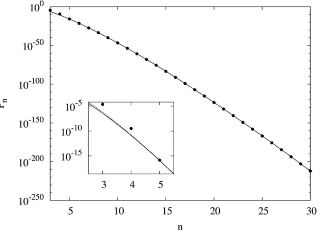
Fig 1shows a semi-log plot of thendependence ofPn. Our estimates ofPnandNnup ton= 30
are listed inTable 1. Exact values for ofNnforn= 3,4 and 5 and the previous estimates ofNn
by Trump for 6n20 are also shown for comparison. We obtainedN30= 6.56(29) × 102056.
In contrast to this extremely large value, its appearance probability,P30, is smaller than 10−212.
Thus the magic squares are numerous but rare.
The largest size ofn= 30 is much larger than that which has been calculated previously. The estimates ofN3,N4, andN5agree with the exact values within the statistical error, and the
there are appreciable discrepancies between the present results and those of Trump forn= 18 and 19; our values are larger for these sizes. In fact, Trump himself pointed out that the true values forN18andN19might be smaller than his estimates based on his own extrapolation
for-mula. We thus think that our estimates are reliable. He also gave estimates ofNnforn>20
ob-tained by the abovementioned extrapolation formula. Compared to the present estimates, his extrapolation results have two-digits accuracy up ton= 30.
As seen inFig 1, the appearance probability of magic squaresPndecreases rapidly withn. In
other words, magic squares become rarer rapidly asnincreases. This raises the question: how fast does their appearance probability decrease? It clearly decreases faster than the exponential function exp(−an) with constanta. On the other hand, since the number of possible
configura-tions isn2!,Pnshould decrease slower than exp(−n2logn). Considering these facts, we first tried
to fit logPnforn10 by the second-order polynomial. But the reducedχ2was larger than 6000 and thus the fitting function was inappropriate. Next we tried functions including logn. The fitting function (An+B)logn+Cn+Dwith the constantsA,B,CandDgaveA=−4.99 ±
0.07 with the reducedχ2= 2.55 and the fitting function (En+F)log(n+G) +Hwith the con-stantsE,F,GandHgaveE=−4.880 ± 0.008 with the reducedχ2= 2.42. Fitted curves using these two functions are shown inFig 1. The two curves are virtually indistinguishable on this scale except for very small values ofn. Other functions we tried gave larger values of reduced Fig 1. Semi-log plot of the appearance probabilityPnof magic squares (•).Pndecreases faster than exponentially with the sizen. Two fitted functions are also shown: exp((An+B)ln(n) +Cn+D) (solid line) and exp((En+F)ln(n+G) +H) (dotted line) withA=−4.99 andE=−4.88. We usedPnofn10 for the fitting. Enlarged plot forn<6 is shown in the inset, in which difference of two functions are visible.
χ2. The reducedχ2for both functions, however, are still large, and the fittings are not fully satis-factory. We consider the reason is thatn= 10 is not yet at the asymptotic region. In fact, when we tried to fit the same functions to data only for larger sizes,n20, we obtained the reduced χ2= 1.30 and 1.37, respectively. Although the errors of the parameters are large,A=−4.6 ± 0.5
andE=−4.88 ± 0.06, reducedχ2for both functions are rather satisfactory.
Fig 2shows the ratioPn/exp{(An+B)logn+Cn+D} andPn/exp{(En+F)log(n+G) +H}.
Both functions seem to expressPnequally well. In any case, since the slope of logPnvaries
slow-ly, it is difficult to determine the appropriate functional form from the present results. We need Pnfor much larger systems to provide a solid conclusion. Even so, we may conjecture that the
logPndecreases asymptotically asanlognwitha’5.
In this paper, we applied the Multicanonical Monte Carlo method to a combinatorial opti-mization problem by defining appropriate an energy functionE(C). The MMC directly gives the number of the optimal configurations from the histogram of the lowest energy
Table 1. Estimated number and qppearance probability of magic squares.
n Pn Nn Trump’s estimates (*exact)
3 2.204(35) × 10−5 0.999(16) 1*
4 3.3645(15) × 10−10 8.7995(39) × 102 880*
5 1.42011(88) × 10−16 2.7534(17) × 108 275305224*
6 3.8182(15) × 10−22 1.77543(73) × 1019 1.775399(42) × 1019
7 4.9955(92) × 10−28 3.7983(70) × 1034 3.79809(50) × 1034
8 3.2931(91) × 10−34 5.223(14) × 1054 5.2225(18) × 1054
9 1.0831(30) × 10−40 7.848(22) × 1079 7.8448(38) × 1079
10 2.069(14) × 10−47 2.414(17) × 10110 2.4149(12) × 10110
11 2.312(12) × 10−54 2.339(12) × 10146 2.3358(14) × 10146
12 1.645(10) × 10−61 1.1417(72) × 10188 1.1424(10) × 10188
13 7.564(61) × 10−69 4.036(32) × 10235 4.0333(54) × 10235
14 2.376(27) × 10−76 1.509(17) × 10289 1.5057(24) × 10289
15 5.082(66) × 10−84 8.00(10) × 10348 8.052(22) × 10348
16 7.933(98) × 10−92 8.50(11) × 10414 8.509(27) × 10414
17 8.898(61) × 10−100 2.313(16) × 10487 2.314(9) × 10487
18 7.500(66) × 10−108 2.146(19) × 10566 2.047(8) × 10566
19 4.657(86) × 10−116 8.37(15) × 10651 8.110(35) × 10651
20 2.216(50) × 10−124 1.773(40) × 10744 1.810(8) × 10744
21 8.34(24) × 10−133 2.589(73) × 10843
22 2.503(73) × 10−141 3.189(93) × 10949
23 5.88(21) × 10−150 3.92(14) × 101062
24 1.099(38) × 10−158 5.85(20) × 101182
25 1.640(44) × 10−167 1.258(34) × 101310
26 2.098(43) × 10−176 4.94(10) × 101444
27 2.150(62) × 10−185 3.86(11) × 101586
28 1.804(74) × 10−194 7.18(29) × 101735
29 1.276(61) × 10−203 3.77(18) × 101892
30 7.78(35) × 10−213 6.56(29) × 102056
Numbers in the parentheses indicate the statistical errors (3 times the standard error) in the last digits.
configurations. The present work demonstrates that the MMC is a powerful tool for counting rare configurations of combinatorial problems. We can estimate the appearance probabilities of the optimal configurations as small as 10−212.
Acknowledgments
We are grateful to Koji Hukushima, Yukito Iba, and Nen Saito for valuable discussions and continuous encouragement. Numerical experiments were carried out on PC clusters at the Cybermedia Center, Osaka University.
Author Contributions
Conceived and designed the experiments: AK MK. Performed the experiments: AK. Analyzed the data: AK MK. Contributed reagents/materials/analysis tools: AK MK. Wrote the paper: AK MK.
References
1. Pickover C (2001) The Zen of Magic Squares, Circles, and Stars. Princeton University Press.
2. Hukushima K, Nemoto K (1996) Exchange Monte Carlo Method and Application to Spin Glass Simula-tions. J Phys Soc Jpn 65 (1996): 1604–1608. doi:10.1143/JPSJ.65.1604
3. Pinn K, Wieczerkowski C (1998) Number of Magic Squares from Parallel Tempering Monte Carlo. Int J Mod Phys C9: 541–546. doi:10.1142/S0129183198000443
Fig 2. The ratio of the appearance probabilityPnto two fitted functions.Pn/exp{(An+B) ln (n) +Cn+D}} (•) andPn/exp{(En+F) ln (n+G) +H} (×) withA
=−4.99 andE=−4.88. Both functions seem to expressPnequally well.
4. Trump W (2005). Available:http://www.trump.de/magic-squares. Accessed 17 December 2014.
5. Iba Y (2001) Extended ensemble Monte Carlo. Int J Mod Phys C12: 623–656. doi:10.1142/
S0129183101001912
6. Berg BA, Neuhaus T (1991) Multicanonical algorithms for first order phase transitions. Phys Lett B267: 249–253. doi:10.1016/0370-2693(91)91256-U
7. Hukushima K (2002) Extended ensemble Monte Carlo approach to hardly relaxing problems. Computer physics communications 147: 77–82. doi:10.1016/S0010-4655(02)00207-2
8. Zhang C, Ma J (2009) Counting solutions for the N-queens and Latin-square problems by Monte Carlo simulations. Phys Rev E79: 016703.
9. Wang F, Landau DP (2001) Efficient, Multiple-Range Random Walk Algorithm to Calculate the Density of States. Phys Rev Lett 86: 2050–2053. doi:10.1103/PhysRevLett.86.2050PMID:11289852
10. Lee J (1993) New Monte Carlo Algorithm: Entropic Sampling. Phys Rev Lett 71: 211–214. doi:10.
1103/PhysRevLett.71.2353.2PMID:10054892
11. Matsumoto M, Nishimura T (1998) Mersenne Twister: A 623-dimensionally equidistributed uniform pseudorandom number generator. ACM Trans on Modeling and Computer Simulation 8: 3–30. doi:10.