A Work Project, presented as part of the requirements for the Award of a Masters Degree in Economics from the NOVA – School of Business and Economics.
ESSAY ON SECULAR STAGNATION
MANUEL CORRÊA DE BARROS DE LANCASTRE
A project carried out on the Research Master in Economics, under the supervision of: Prof. Francesco Franco
Essay on Secular Stagnation
Abstract
In this paper we show that a closed economy, with a balanced budget and unable to increase public spending, can avoid or leave a persistent slump through adequate and timely combination of monetary and fiscal policy based on distortionary taxation. We use a three generations OLG New Keynesian model in which a permanent slump is possible without any self-correcting force to full-employment. Complementing recent work on Secular Stagnation using lump-sum taxation and government spending as fiscal instruments, our contribution is to use distortionary taxes over labor, consumption and capital, in a balanced budget environment with constant (or decreasing) government spending.
1 Introduction and literature review
During IMF 14th annual research conference in November 2013 Larry Summers resurrected the expression “Secular Stagnation” firstly used in 1939 by Alvin Hansen, the President of the American Economic Association, where he stated that the Great Depression could be the start of an era of economic stagnation and of permanent and significant level of unemployment. An oversupply of savings and a low birth rate were then considered relevant causes of a restrained aggregate demand. Analogously, Summers suggests that similar conditions could be applied to the US after 2008, and could have been in place well before the crisis, although disguised by the recent housing bubble. The case of Japan during the last 20 years of economic stagflation may well also be regarded as part of the same phenomena, as referred by Krugman in the New York Times two months before Summers speech, where he mentioned that the “secular stagnation” hypotheses could be a natural epilogue of his research on the “liquidity trap”. Furthermore, in his recent book, “Le capital au XXIe siècle”, Piketty argues that the generous growth rates of output per capita during the period between 1970 and 2010 were one of a few exceptions in human history, and that we should expect growth rates not much greater than 1% during this century.
be insufficient to achieve simultaneously full-employment, growth and financial stability, as economic bubbles, for example, become more likely in environments of low nominal interest rates, high propensity for savings, and low demand for loans.
Factors like higher borrowing restrictions from financial institutions due to financial crisis, or lower birth rates, contribute to lower demand for loans, creating a downward pressure on interest rates. In the loans market supply side, financial crisis increase the need and propensity for households, companies, and financial institutions to invest in safe assets rather than in riskier ones (see Caballero and Fahri 2014). Moreover, a decreasing trend of the relative price of durable goods, and thus of the cost of investment, leaves more funds left for savings, also creating a downward pressure on interest rates. Furthermore, when inflation is low, nominal wage rigidities may create an upward pressure on real wages further depressing output as well as the natural rate of interest consistent with full-employment. Nominal interest rate zero lower bound together with low inflation may prevent real interest rate to decrease to the level of the natural rate of interest, thus creating the conditions for a permanent slump. Explaining secular stagnation and its causes is the purpose of a recent paper by Eggertson and Mehrotra (2014) who propose a model where a slump is possible without any self-correcting force to full-employment, and where public spending together with lump-sum taxes are used as fiscal policy instruments.
2 Description of the closed economy model
The simple OLG model we propose allows for steady state equilibriums with persistent negative real interest rates, when population growth is low enough or when credit constraints are present. We will present the model starting with (i) a simple endowment economy with population growth, (ii) adding credit constraints, (iii) endogenous output, (iv) fiscal policy, (v) monetary policy, and (vi) capital.
Endowment economy:
In the model, households go through three stages of life: young, middle aged and old. The young generation borrow from the middle aged; the middle aged save by lending to the young, and pay back their loans to the previous generation, then old. The old receive back with interest what they have lent to the young when middle aged. Lending is constrained by a binding debt limit faced by the young, exogenously determined and independent of any fiscal instrument. For simplification, income is only earned by the middle aged. For this simple endowment economy the household objective function and budget constraints are given below:
max , , log + log + log (1)
s.t. = " (2)
= # − 1 + & " − " (3)
= 1 + & " (4)
Furthermore, loan market equilibrium implies that total borrowing of young generation equals total savings of middle aged, or ' " = '( " , where ' is the size of
generation t. Then 1 + ) " = " (5)
where ) = ' /'( is population growth. For constant endowment the equilibrium level real interest rate is given by 1 + & = 1 + ) / , which can be negative if
Adding Credit Constraints to the model:
By adding a lending constraint through an exogenously determined binding borrowing limit faced by the young, 1 + & " ≤ - (6) we get an expression for the borrowing of the young " , and savings of the middle aged
" given by " = .
/ 00000and00000" = 3
/ - 00000000000000000000000000000000000000000 7
and an equilibrium real interest rate, which can be negative, given by the expression:
1 + & =01 + 1 + ) -# −
-( 000000000000000000000000000000000000000000000000000000000000 8
(iii) Introducing Endogenous Output into the model
Expression (8) does not change when we add endogenous output to the model, by replacing constraint (3) by: = 67 + 8 9 : − 1 + & " − " 000000000 9 Where, for now, the firm problem has no capital and is given by:
< = max0= # −8 9 00000s. t000000000#AB 9 C, then08 = F9 0000000000000000000000000 10#
At full employment 9 = 9H and #I = B 9HC. For simplicity we assume B = B = 1.Then
#Iis constant, which will not be the case when capital is introduced in the model. From (8), we can derive the expression for demand output:
#J =0K1 + L 1 + )
-1 + & + -( 000000000000000000000000000000000000000000000 11
And we can establish an expression for the real interest rate for a full employment equilibrium, which we will call the natural rate of interest0&I:
1 + &I =0K1 + L #1 + ) -I−
-( 000000000000000000000000000000000000000000000000 12
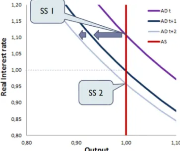
Figure 1: Demand output, and full-employment real interest rate
3. Fiscal policy with distortionary taxation
In this chapter we introduce distortionary taxation into the model, derive expressions for demand and real interest rates, and analyze how those are affected by tax changes in this closed economy with borrowing constraints and a balanced budget. We will see how adequate fiscal policy may offset the recessionary effects of an increase of credit constraints. In Eggertson and Mehrotra’s model taxes are lump-sum and paid by middle-age households. Firms don’t pay taxes and household constraints are given by:
= " − N (13)
= 7 + 8 9 − 1 + & " − " − N (14)
= 1 + & " − N (15)
taxes for average middle aged households are given by0N = PQ + PR8 9 . Firms pay taxes on labor costs: NST = PST8 9 . Euler equation is now given by:
1 + & = 1 1 + P1 + PQQ U 000000000000000000000000000000000000000000000000000000 16
Combining the Euler equation with the constraint given by expression (15) we get
" = WX / = 1 + PQ , or = Y
Z WX . From loan market equilibrium (5), and the borrowing constraint (6) we get expressions for household consumption:
=1 + P1 QK1 + & L - ;01 =1 + P1 QK1 1 + )1 + & L - ;0 = 1 + P1 Q 1 + ) ( -(
Total consumption in period t is given by: \ ]R = ' + ' + '( , from which the expression for total consumption per middle aged household is derived:
= 1 + ) + + 1 + ) =1 + P1 Q^K1 + L 1 + ) -1 + & + -( _00⟺
1 + PQ = K1 + L 1 + )
-1 + & + -( 00000000000000000000000000000000000 17
An expected result in this binding credit constrained closed economy, where equilibrium consumption is a negative function of consumption tax. Then, from (17), assuming a balanced budget,0N = O , and using market clearing condition for goods,
# − = O , expressions for demand and real interest rate are given by:
#J = + O = 1
1 + PQ^K1 + L 1 + ) -1 + & + -( _ + O 00000000000000000000 18
1 + & =0K1 + L 1 + PQ 1 + ) -# − O −
-( 0000000000000000000000000000000000 19
#J = K 1
1 − Fa L ^K1 + L 1 + ) -1 + & + -( _ = 1 + P
Q
1 − Fa , with0a =P
ST+ PR
1 +0PST0 20
1 + & =0K1 + L 1 − Fa # − -1 + )
-( 000000000000000000000000000000000000 21
Equivalence of aggregate demand expressions (18) and (20) under a balanced budget indicates that, with constant public spending, an increase in labor taxes gives room for reducing consumption taxes which will cause a demand expansion. This statement points to a relation between fiscal instruments and aggregate demand, illustrated by expression (22) derived from the above two alternative expressions for0#J, together with the expression for total taxes per middle aged household:
N = PQ +(PST+ PR 08 9 0=0PQ + Fa # 0=0dWX Ce
0WX f #J0= g1 − d (Ce
0WXfh #J00=
= 0#J− = O when the budget is balanced. This equality is equivalent to:
O
#J = 1 − i1 − Fa1 +0PQ j ⟺ 0#J = O P Q+ 1
PQ + Fa 0⟺ 0a =1F ^O − P
Q #J− O
#J _000 22
Any equality in expression (22) works like a “Taylor rule” for fiscal policy that ensures the budget is balanced on a period by period basis. We will call it the fiscal rule, which implies that at least one fiscal instrument is endogenously determined. For the time being we will assume this is the case for0a = Wkl0WklWm0. Moreover, labor supply is inelastic which, at full employment, makes taxes on labor non-distortionary.
As seen in previous chapter, full employment can be kept after a credit shock or a reduction of population growth as long as the real interest rate sticks to the natural rate of interest, now given by expression below, due to the distortionary taxation setting:
1 + &I= K1 + L 1 + ) -1 + PQ #I− O −
-( = K
1 +
L 1 + )
-1 − Fa #I− -( 000 23
lower bound for nominal interest rates together with a low inflation level. Full-employment equilibrium remains possible if the natural rate of interest increases back to an admissible real interest rate level, through a reduction of the consumption tax compensated by an increase of labor taxes in order to fulfill the fiscal rule given by expression (22). This would shift back to the right aggregate demand so that the intersection with full employment supply curve # = #I moves up to an admissible real interest rate level so that a full employment equilibrium persists and a secular stagnation is avoided. The purpose of the next chapter is to analyze how to avoid a slump using fiscal and monetary policy.
4 Avoiding a Secular Stagnation
To avoid a liquidity trap, caused by a credit shock or a reduction of population growth, policy makers have a combination of two options: (i) To increase back with fiscal policy full-employment real interest rate &I, if the real interest rate cannot be sufficiently reduced. (ii) Or alternatively, to unblock with monetary policy the required reduction of the real interest rate to the new lower level of the natural rate of interest &I. Let’s start by analyzing the first option, in a model with constant prices and flexible wages.
4.1. Avoiding a slump with fiscal policy 4.1.1. Constant prices and flexible wages
(23), all other parameters constant excepting taxes, full employment level is kept in steady state 2 if:
&I = &I = & 000⟺000001 + P1 + PQQ =
-- =
1 − Fa
1 − Fa ,0000000where0a =0
PR+ PST
1 +0PST000000000000 24
This states that a reduction of the borrowing limit can be compensated by a decrease in consumption taxes in order to keep constant the natural rate of interest. A reduction of the borrowing limit would shift the demand curve to the left, reducing the natural rate of interest, which could become lower than the lower admissible real interest rate level, causing a slump. But a sufficient reduction of consumption tax would neutralize the previous effect by moving back the demand curve to its previous position, thus increasing the natural rate of interest0&Iback to its initial level0&I. Increasing one of the labor taxes, or both, is required to fulfill the fiscal rule. This process may be helpful in a model with nominal prices and nominal interest rates zero lower bound, when the natural rate of interest can become smaller than the real interest rate lower admissible level limit.
4.1.2. Introducing nominal price determination in the model, with flexible wages
From now on nominal prices are considered as in Eggertson and Mehrota’s model, where nominal interest rate follows the Taylor rule. The household problem maximization constraints are given by:
q 1 + PQ = q " (25)
q 1 + PQ = < + r 9 1 − PR − 1 + s q " + q " (26)
q 1 + PQ = − 1 + s q " (27)
And the Taylor rule: 1 + iu = max v10, 1 + sw dxxwfyz{ , where |} ~ 1 (30)
The Euler equation is now given by: =
Z d
WX
WX f • t
t 00000000000000000 31
Factors in “t + 1” are canceled due to the loan market equilibrium and the borrowing limit for the young, and expressions for aggregate demand and real interest rates are the same as the ones derived in chapter 3 (see appendix).
Using the Taylor rule combined with the Fisher equation we get the following alternative expression for the real interest rate:
1 + & = 1 + s€ = •B‚ ƒ€ 0,1 1 + s€w wK€€wLyz( „ … 1 + s€ww yz = 1 + &†•‡†000 32
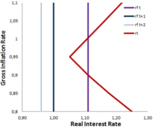
If &Ibecomes lower than &†•‡† (figure 2) after a credit shock then a full-employment equilibrium is not allowed, unless a sufficient consumption tax reduction (offset by an increase of other taxes) compensates for the decrease of the borrowing limit, as seen in previous chapter.
Figure 2: real interest rate function of inflation, and natural rate of interest
compensated by an increase of labor income tax by more than 10 percentage points. Although theoretically possible, trying to avoid a slump in such conditions using fiscal policy only, when government spending cannot increase, may be difficult to achieve. Monetary policy can then be a complement or an alternative, if available.
4.2. Avoiding a slump with monetary policy Still with flexible wages…
To allow a full-employment equilibrium, an alternative to fiscal policy is to decrease the real interest rate lower bound &†•‡†to a level lower than the natural rate of interest0&I.
&†•‡† = x•w Šzw − 1 is a function of monetary policy instruments, namely target
inflation and target nominal interest rate. Since target nominal interest rate is positive because of ZLB, then &†•‡† is smaller than the target real interest rate &w = x•ww − 1: Then &wbelongs to the set of admissible equilibrium real interest rates, as proven below:
1 + &†•‡† = 1 + sw yz
€w =1 + s w
€w 1 + sw yz( ≤ 1 + &w 00000for00sw … 0, |} … 1000 33
For sw = 0 , &†•‡† = &w, whereas a negative &w implies a positive inflation target
1 ≤ /w ≤ €w. Furthermore, the Taylor rule for Π … 10is equivalent to0d //wf =
remain fully consistent with the new lower natural rate of interest&I, by decreasing sw and increasing €w, as seen in figure 3.
Figure 3: real interest rate function of inflation, and natural rate of interest
Deriving Aggregate Supply and equilibrium output when wages are sticky
In this model, when wages are sticky and the natural rate of interest becomes negative because of a credit shock or a decreasing population growth, then a unique determinate secular stagnation equilibrium becomes available. A timely and assertive reaction of policy agents is of primal importance to prevent the economy from diving into a slump. Sticky wages are introduced in the model as in Eggertson and Mehrotra (2014): Households will not accept working for a wage lower than a nominal wage norm rŽ given by rŽ = •r( + 1 − • q 8IR•‘, whereas nominal wage will allways be greater or equal than the flexible labor full-employment nominal wage:
r = max rŽ , q 8IR•‘ , where 8 =’t = CWkl “= = C]”“
”• ”
Wkl , and 8IR•‘= C“–”•”
Wkl
for B = 1. The short term AS curve is given by:
#C(C = max ƒ 1 + PST
1 + PST( Π #• ( C(
C + 1 − • # I
C( C , #
I C(
C „0000000000000000000 34 0
#SSe—0˜•3˜ = #I, for0Π … 1;000000Π = 1 − 1 − • i• #e—0R ™#
I j
(C C
, for0Π < 1000 3š
This expression is independent of PST and all other fiscal instruments. For negative inflation, supply is and upward sloping function of inflation.
Moreover, we get the aggregate demand #J0function of inflation by replacing the real interest rate expression (32) in the aggregate demand expression (18), given by:
#J =
› œ • œ
ž0#J0˜•3˜ =0 1
1 + PQ^ 1 + 1 + ) - 0Π†•‡† yz
Π yz( + -( _ + O 0, Π ~ Π†•‡† 36
0#J0R ™0=0 1
1 + PQ^ 1 + 1 + ) - 0Π 00000000000+ -( _ + O 0, Π ≤ Π†•‡† 37
Where Π†•‡† = •w •w |Ÿ=
•w|Ÿ|Ÿ•
/w |Ÿ
.
As discussed in previous section, sustaining a full employment equilibrium when &I becomes negative and fiscal policy cannot raise it back to a positive level, may require that monetary instruments stay consistent with monetary variables. (see figure 4 below).
. Figure 4: Avoiding a slump with monetary policy, and sticky wages
This means that &w = &I < 0 and Πw ~ 1 because sw is not negative. In that case
Π†•‡† ~ 1. Moreover Π†•‡† = Πw for sw = 0. For Π = 1 < Π†•‡† , 1 + & =
1 + &I then # Π = 1 < #I meaning that the lower AD segment crosses the vertical line # = #I at Πe.0IR•‘0~ 1, when lower AS segment crosses the same vertical line at0Π = 1. This is going to be important in the next chapter, besides being a crucial step to prove that there is a unique determinate secular stagnation equilibrium in the model. From figure 4 we can infer that if &I becomes negative, lack of assertiveness or consistency from fiscal and monetary policy agents may clear the full-employment equilibrium leaving the economy, even during a short period, only with a secular stagnation one, from where it is difficult to get out. This can have been the case in Europe when the ECB decided to increase the interest-rate targets in 2008 right after the Lehman Brothers crash, and in 2011 during the credit crash, which could have triggered and consolidated the creation of a stable and persistent liquidity trap in EU, where sw can no longer be reduced and Πw is not increasing for political matters. Leaving a slump is the purpose of the next chapter.
Figure 4: ECB interest-rate targets
5 Leaving a Deflationary stable equilibrium
monetary policy is ineffective to clear from the model a secular stagnation, but may be a relevant tool in order to allow for a full employment equilibrium in the model to where the economy may migrate.
5.1. Eliminating a secular stagnation stable equilibrium
A secular stagnation is characterized by the intersection of the lower segments of AD and AS curves. None of those two expressions (35) and (37) depend on monetary policy instruments. Moreover the long term steady state expression for aggregate supply for negative inflation does not depend on fiscal instruments either. So the only way to clear a secular stagnation steady state is to ensure that lower AD intersects aggregate supply at full employment output, which corresponds to a zero inflation level for aggregate supply. As in previous chapter, let Πe.0IR•‘~ 10be the gross inflation level where the line given by expression (37) corresponding to the lower AD segment intersects the vertical full employment line. To clear a secular stagnation steady state Πe.0IR•‘ must change from Πe.0IR•‘~ 10to Πe.0IR•‘ = 1, which requires a consumption tax change, derived from expression (23) and (24), given by (proof in appendix (A.6):
∆PQ = 1 + PQ
Πe.0IR•‘+ 1¡ 1 − Π
e.0IR•‘ 0,000000where000000¡ = 1 + 1 + ) 000000000 37
Because Πe.0IR•‘~ 1, the consumption tax change corresponds to a tax reduction that will increase the natural rate of interest sufficiently to clear-up the secular stagnation as in chapter (4.1). Labor taxes must increase to fulfill the fiscal rule (22), and monetary policy must ensure that demand gross inflation kink is greater than one to allow for a full-employment equilibrium in the model.
But by acting over the short run aggregate supply given by expression (34), through and adequate change of the labor tax on firms PST, the liquidity trap equilibrium can be eliminated at least for one period:
During a secular stagnation steady state, both short term and long term lower AS segments intersect lower AD segment for #SS < #I and ΠSS < 1. Similar to the previous section, to eliminate a slump equilibrium at least for one period, we need lower AD, and now lower short term AS segments to intersect at full employment output, for
#SS = #I. Based on expression (34) short term aggregate supply intersects full employment vertical line at an inflation level Πe—,I given by:
Πe—,I PST = 1 + PST
1 + PST( i##(I j C(
C
0000000000000000000000000000000000000 38 0
We then need at least a shift of lower AS or of lower AD so that Πe—,I = Πe.,I, where
Πe.,Iis the intersection of AD lower segment with full employment for the period when the slump is supposed to be cleared. This requires a change of firm labor tax PST given by expression below, derived directly from expression (38):
1 + PST
1 + PST( =ΠSS e.,I
ΠSSe—,I i Πe.,I
ΠSSe.,Ij =0⟺0∆PST = 1 + PST( i Πe.,I
ΠSSe—,I − 1j000000000000 39
Where ΠSSe.,I and ΠSSe—,I are inflation levels corresponding to the intersections of lower AD and AS respectively with full employment line when the economy is in a secular
stagnation equilibrium. Directly from expression (38), ΠSSe—,I = d“kk “–f
”• ”
= ¢SS”•” ~ 1.
ΠSSe—,I0 is high for low secular stagnation output levels, or more depressive slumps. Expression (39) can then also be written as:
1 + PST
1 + PST( = Πe.,I¢SS (C
If lower AD segment remains unchanged, then Πe.,I = ΠSSe.,I, and ∆PST has positive or
negative sign depending on the relation between ΠSSe.,I and ΠSSe—,I = ¢SS”•” .
(i) If0ΠSSe—,I ~ ΠSSe.,I, or equivalently when ¢SS < ΠSSe.,I
”
•” when the slump is deeper,
then ∆PST < 0 stating that a supply expansion driven by a reduction of labor tax on firms is necessary to eliminate the liquidity trap for one period. In that period the economy should move to the full-employment equilibrium that adequate monetary policy should ensure. Although the short term AS curve will return to its steady state shape on the following period, the economy might be able to sustain itself on the full-employment equilibrium. Alternatively, an adequate demand contraction through an increase of consumption tax, ∆PQ ~ 0, would raise Πe.,I from ΠSSe.,Ito Πe.,I ~ ΠSSe.,I, and could have the same effect of clearing the slump for one period, if monetary policy ensures that Y†•‡† ~ YI. But changing both taxes in opposite directions may be easier to implement than changing just one of them: Only increasing PQ may help eliminate a slump in the short term but will deepen the available secular stagnation equilibrium in the model; moreover it may call for monetary policy intervention in order to ensure a full employment equilibrium to where the economy can migrate; monetary policy instruments might not be available. A reduction of PST without increasing PQ might need to be too assertive, calling for an also too assertive increase of PR in order to fulfill the fiscal rule (22); although this would avoid the deepening of the steady state slump available in the model, the higher assertiveness of the changes in particular of labor income taxes could be politically difficult to sell. An adequate combination of a smaller
(ii) Otherwise, if ΠSSe—,I < ΠSSe.,I , or equivalently when ¢SS ~ ΠSSe.,I
”
•” for lighter
slumps, a supply contraction through an increase of labor tax on firms PST, could clear the deflationary equilibrium for one period. This can be explained mentioning the paradox of toil, illustrated by Eggertson (2014), stating that an aggregate supply expansion can have contractionary effects when an economy is in a liquidity trap, by triggering deflationary pressures that raise the real interest rate 1 + & =
• and further depressing demand. The key behind this is a lower AD segment positive slope, higher than the slope of the lower AS segment. In order to fulfill equation (22) and keep AD curve unchanged, income labor tax on households must be reduced. Alternatively a further demand expansion through a consumption tax reduction would have a similar effect, and could be, in that situation, a safe complement or alternative.
Figure 5: Using labor tax on firms
6. Introducing Capital and a Tax on Capital in the model
households P† can be a relevant fiscal policy instrument as alternative or a complement to consumption tax changes, in order to avoid, to clear, or migrate from a liquidity trap. Aggregate demand: Constraints (26) and (27) of household problem with capital in real terms are given by:
1 + PQ = 7 + 8 9 1 − PR + ¤ &† 1 − P† − 1 − 1 + & " + " 0000000 41
1 + PQ = − 1 + & " + ¤ 1 − ¥ 0000000000000000000000000000000000000000000000000000000000 42
First order condition for K is given by: FOC0¤ :0&† =
(Wª d1 − («
/f000000000000000000 43
Firm problem: 7 = max
= # −8 9 1 + PST − &†q ¤ 00s. t00#AB 9
C¤ (C000000000000000 44
Now08 = C=”•Wkl = CWkl =“ and000&† = 1 − F a 9 C¤(C( = (C “¬ . Aggregate Demand has now the expressions below:
#J =0i 1
1 − Fa − 1 − F "Rj ^K1 + L 1 + ) -1 + & − -( _00000000000 4š
or0000#J =0i 1
1 + PQ − 1 − F "Qj ^K1 + L 1 + ) -1 + & − -( + O 1 + PQ _0000000 46
Where "R = /ªd
Z Z f
(«
/ « = 1 − P† d Z Z f
(«
/ « , and "Q =/ªd1 + PQ¥ +Z («
/ f.
From expression (43) we can observe that &† decreases when P† is reduced, and from (45),(46) that a reduction of P†has an expansion effect on #J through a reduction of &†. Aggregate Supply: Expressions for aggregate supply are similar to the model without
capital: #S = #I for Π … 1, and 0•- = 1 − 1 − • K““
–L •” ”
for Π < 1. The difference lies on the supply expression for positive inflation levels which is not constant, and expands with P†reductions:
#I = B 9HC¤ (C = 9HB /Ci1 − F
&† j (C C
= 9HBC® 1 − F 1 − P†
1 − 1 − ¥1 + & ¯
(C C
Then the lower AS segment also shifts out with a reduction of P†, and the kink of AS curve is a negative function of capital tax, and is maximized at P† = 0:
0#e—0¬•‡† = 9HB /C^ 1 − F 1 − P†
¥ _
(C C
≤ 9HBC°1 − F
¥ ±
(C C
000000000000000 48
Secular stagnation equilibrium: A reduction of tax on capital expands both aggregate demand and aggregate supply. When the economy is in a steady state secular stagnation, a shift out of aggregate supply has deflationary effects (see paradox of toil in Eggertson 2014), and a shift out of aggregate demand has inflationary effects. The net effect of a
P† reduction is an increase in inflation and output equilibrium levels (proof available), which makes P† an alternative or a complement to consumption tax changes to avoid, to clear, or to migrate from a liquidity trap. To clear a liquidity trap from the set of possible determinate equilibriums (see chapter 4) a decrease of P† can be used as an alternative to a decrease of consumption tax, or as complement. To migrate to a full employment equilibrium (chapter 5) changes of P† although having a similar effect than changes of PQof the same sign, should be managed more carefully as they trigger shifts of AS and AD in the same direction, and may attenuate the effect of PSTchanges. In any case, decreasing P†alone (compensated by increasing any of the labor taxes) will expand equilibrium output, and may mitigate, although not clear, a secular stagnation.
7. Conclusion
References
Caballero, Ricardo, and Emmanuel Farhi. 2014. “The Safety Trap.” National Bureau
of Economic Research.
Chari, Kehoe. 2006. “Modern Macroeconomics in Practice: How theory is shaping policy”. National Bureau of Economic Research.
Chari, Christiano, Kehoe. 1991. “Optimal Fiscal Policy and Monetary Policy: some recent results”. Federal Reserve Bank of Minneapolis and University of Minnesota Eggertson, Gauti B, and Neil R. Mehrotra. 2014. “A Model of Secular Stagnation”
Mimeo, Brown University.
Hansen, Alvin. 1939. “Economic Progress and Declining Population Growth.”
American Economic Review, 29(1): 1–15.
Krugman, Paul R. 1998. “It’s Baaack: Japan’s Slump and the Return of the Liquidity Trap.” Brookings Papers on Economic Activity, 2: 137–205.
Krugman, Paul R. 2013. “Bubbles, regulation, and secular stagnation.” The New York
Times Blog,25 September
Summers, Lawrence. 2013. “US Economic prospects: Secular Stagnation, Hysteresis and the Zero Lower Bound.” Business Economics, Vol. 49, No.2
Summers, Lawrence. 2013. “Why Stagnation Might Prove to be the New Normal.”
The Financial Times.
APPENDIX
A.1. Household problem
max , , log + log + log , s.t. (H.1)
q 1 + PQ = q " (H.2)
q 1 + PQ = < + r 9 1 − PR − 1 + s q " + q " (H.3)
q 1 + PQ = − 1 + s q " (H.4)
And an exogenous borrowing limit: 1 + s q " ≤ q - (H.5) Let’s use the Fisher equation: 1 + s = 1 + & tt (M.1) Replacing (H.2), (H.4), (H.5) and (M.1) in (H.3), and diving (H.3) by q we get:
1 + PQ + WX
/ =²t + 8 9 1 − PR − - (H.3.1)
From (H.1) s.t to (H.3.1) we obtain an Euler equation:
−" = WX/ = 1 + PQ (H.6)
And replacing (H.6) in (H.3.1) we get:
1 + 1 + PQ = ²
t + 8 9 1 − PR − - (H.3.2)
A.2. Firm problem
< = max= q # −r 9 1 + PST 00000s. t000000000#AB 9 C (F.1)
Then:0008 =’t =C] =W”•kl = CWkl =“ =C] ”“”•”
Wkl (F.2)
A.3. Equilibrium in the bond market
' " = −'( " ⇔ 1 + ) " = −" ⇔ 3/ - = −" (B.1)
By replacing (H.6) in (B.1) we get: 3
/ - = 1 + PQ (B.2)
Using the Taylor rule: 1 + s = max{10, 1 + sw d••wfyz} (M.2) Combining with the fisher equation:
1 + & = · 1 + &w d
• •wf
yz(
= • d••ª¸¹ªfyz , Π ~ Π†•‡†
• 0000000000000000000, Π ≤ Π†•‡†
0 (M.3)
A.5. Aggregate Demand
Using (F.1) and (F.2), ( H.3.2) can be rewritten as:
1 + 1 + PQ = # 1 − Fa − - ;0000a = Wm Wkl
Wkl (D.1)
And now replacing (B.2) in (H.3.3) we finally get the expression for aggregate demand:
# =0K1 − Fa L ^K1 1 + L 1 + ) -1 + & + -( _00000000000000000000000000000000 D. 2
and for the real interest rate:
1 + & =0K1 + L 1 − Fa # − -1 + )
-( 000000000000000000000000000000000000 D. 3
Replacing the real interest rate by (M.3):
Π†•‡† = Π w
1 + sw |Ÿ
00, and0#†•‡† = K1 − Fa L ^1 1 + 1 + ) - Π†•‡† + -( _ -. 4
And the expression of Aggregate Demand, # = # Π :
# = › œ • œ
ž0#˜•3˜ =0K 1
1 − Fa L ^ 1 + 1 + ) - 0Π†•‡†
yz
Π yz( + -( _0, Π ~ Π†•‡†00 -. š
0#R ™0=0K 1
1 − Fa L ^ 1 + 1 + ) - 0Π 00000000000+ -( _0, Π ≤ Π†•‡†000 -. 6
In steady state - = -( =
-# =0K1 − Fa L ^K- 1 + L 1 + )1 + & + 1_00000000000000000000000000000000 D. 7
1 + & =0K1 + L 1 − Fa # − - 000000000000000000000000000000000000 D. 81 + )
1 + &I =0K1 + L 1 − Fa #1 + )
-I− - 000000000000000000000000000000000000 D. 9
If 1 + &w = 1 + &I0then0there0is0and0equilibrium0in0the0model0where0Π = Πw0. In particular if iw= 00then0Π = /
–= Π
w = Π†•‡†0and0Y†•‡† = 0YI00
A.5. Aggregate Supply
r = max rŽ , q 8IR•‘ 0where0rŽ = •r( + 1 − • q 8IR•‘000000000000000 AS. 1
8 = max 8À , 8IR•‘ 0where08À = •8Π + 1 − • 8( IR•‘0000000000000000000000 AS. 2
FBC#C(C
1 + PST = max
› œ • œ ž •
FBC( # ( C(
C
1 + PST(
Π + 1 − •
FBC#IR•‘C(C
1 + PST( ,
FBC#IR•‘C(C
1 + PST(
Á œ  œ Ã
00000 AS. 3 0
Assuming for simplicity that a is constant in time,
#C(C
1 + PST = max
› œ • œ ž •
#C((C
1 + PST(
Π + 1 − •
#IC(C
1 + PST ,
#IC(C
1 + PST
Á œ  œ Ã
0000000 AS. 4 0
#C(C = max ƒ 1 + PST
1 + PST( Π #• ( C(
C + 1 − • # I
C( C , #
I C(
C „00000000000 AS. š 0
Then the lower part of the AS curve has the following expression for 0Π :
•
0Π = i1 + P (
ST
1 + PSTj ÄK## L( (C C
− 1 − • i##(
I j (C C
Å00000000000000 AS. 6
In steady state (with constant taxes) AS curve is independent of PST:
•
0Π = 1 − 1 − • i##Ij (C C
00000000000000000000000000000000000000000000000 AS. 7
In order to avoid an intersection of the lower part of AD curve with the lower part of AS curve in steady state it is sufficient to move AD curve so that it intersects the AS curve at # , 0Π = #I, 1 : #J ΠI, PQ = #I = #J ΠI, PQ
•–A
ÆÇÈ
-1 + PQ^ 1 + 1 + ) ΠI+ 1_ + O =1 + P- Q^ 1 + 1 + ) ΠI+ 1_ + O •ÆÇÈ–A
1 + PQ
1 + PQ =¡Π¡ + 1I+ 1, ¡ = 1 + 1 + ) •ÆÇÈ0∆P–A Q =
1 + PQ
ΠI+ 1¡ 1 − Π
I 00000000000 9N. 1
A.5. Migrating from a liquidity trap to a positive inflation equilibrium From (AS.6), the lower part of the AS curve intersects # = #I at0ΠI :
0ΠI = i1 + P1 + PST
(
ST j K##I ( L
(C C
⟺ i1 + P1 + PST
(
ST j = 0ΠI¢( (C
C 0where0¢( =#(
#I 0
This can be written like: ∆PST = PST − PST( = 1 + PST( ΠI¢(
•” ” − 1
B. Derivation of the Model with Capital B.1 Household problem
q 1 + PQ = < + r 9 1 − PR − q ¤ + q ¤ &† 1 −
P† − 1 + s q " + q " (CH.3)
q 1 + PQ = − 1 + s q " + q ¤ 1 − ¥ (CH.4)
1 + PQ + WX
/ =
²
t + 8 9 1 − PR + ¤ g−1 + &† 1 −
P† + («
/ h − - (CH.3.1)
FOCs revisited:
FOC0 :0 WX/ = 1 + PQ (CH.6)
FOC0¤ :0&† =
(Wª d1 − («/f (CH.7)
< = max= q # −r 9 1 + PST − &†q ¤ 00000s. t000000000#Aa 9 C¤ (C (CF.1)
Then:0008 =’t = C=”•Wkl = CWkl =“ (CF.2)
and:000&†= 1 − F a 9 C¤(C( = (C “
¬ (CF.3)
Then ( CH.3.1) can be rewritten as:
1 + 1 + PQ = # 1 − Fa − ¤ ^1 − 1 − P† &†− 1 − ¥
1 + & _ − -( CH. 3.2
Where a = Wm WWklkl
B.3. Equilibrium in the bond market
' " = −'( " ⇔ 1 + ) " = −" ⇔ 3/ - = −" (CB.1)
From (CH.4): −" =0 WX / − ¤ («/ (CB.2)
⟺ 1 + PQ =0 1 + ) - + ¤ 1 − ¥ (CB.2.1)
Replacing (CH.6) in (CH.4): −" = 0 1 + PQ − ¤ («/ (CB.3)
By replacing (CB.1) in (CB.3) we get: 3
/ - + ¤
(«
/ = 1 + PQ (CB.4) B.4. Aggregate Demand
Inserting (CB.4) in (CH3.2) we get: Z
Z g 3/ - + ¤ («/ h = # 1 − Fa − ¤ g1 − 1 − P† &†− («/ h − -( ⟺
⟺ 0# 1 − Fa = -( + 1 + 1 + )1 + & - + ¤ i1 +1 1 − ¥1 + & − 1 − P† &†j
And replacing: ¤ = (C “
/ª we get:
# =0K1 − Fa − 1 − F " L ^K1 1 + L 1 + ) -1 + & + -( _00000000000000000000 CD. 1