the requests in eachGw , w ¼ 1, . . . ,W, can be routed through arc disjoint paths in G. The paper is structured as follows. In the next section we discuss related works in the literature. In Section 3 we describe the VND-ILS heuristic for the min-RWA. Th

(1)

Variable neighborhood descent with iterated local search for routing and

wavelength assignment

Alexandre X. Martins

a,b

, Christophe Duhamel

c

, Philippe Mahey

c

, Rodney R. Saldanha

d

,

Mauricio C. de Souza

e,n

a_{Programa de Po}_´s-Graduac

-ao em Engenharia Ele´trica, Universidade Federal de Minas Gerais, Av. Antˆ~ onio Carlos, 6627, cep: 31270-901, Belo Horizonte, MG, BraZil b_{Departamento de Ciˆencias Exatas e Aplicadas, Universidade Federal de Ouro Preto, Jo}_{ao Monlevade, MG, Brazil}~

c_{Laboratoire LIMOS, CNRS-UMR 6158, and ISIMA, Universite´ Blaise Pascal, Campus des Ce´zeaux, BP 10125, 63173 Aubi}_{ere CEDEX, France} d_{Departamento de Engenharia Ele´trica, Universidade Federal de Minas Gerais, Av. Antˆ}_{onio Carlos, 6627, cep: 31270-901, Belo Horizonte, MG, Brazil} e_{Departamento de Engenharia de Produc}

-~

ao, Universidade Federal de Minas Gerais, Av. Antˆonio Carlos, 6627, cep: 31270-901, Belo Horizonte, MG, Brazil

a r t i c l e

i n f o

Available online 17 November 2011

Keywords:

Routing and assignment Network design

Variable neighborhood descent Local search

a b s t r a c t

In this work we treat the Routing and Wavelength Assignment (RWA) with focus on minimizing the number of wavelengths to route demand requests. Lightpaths are used to carry the trafﬁc optically between origin-destination pairs. The RWA is subjected to wavelength continuity constraints, and a particular wavelength cannot be assigned to two different lightpaths sharing a common physical link. We develop a Variable Neighborhood Descent (VND) with Iterated Local Search (ILS) for the problem. In a VND phase we try to rearrange requests between subgraphs associated to subsets of a partition of the set of lightpath requests. In a feasible solution, lightpaths belonging to a subset can be routed with the same wavelength. Thus, the purpose is to eliminate one subset of the partition. When VND fails, we perform a ILS phase to disturb the requests distribution among the subsets of the partition. An iteration of the algorithm alternates between a VND phase and a ILS phase. We report computational experiments that show VND-ILS was able to improve results upon powerful methods proposed in the literature.

1. Introduction

Optical networks with wavelength division multiplexing (WDM) provide users with very large bandwidths. In all-optical networks a traffic demand is carried from source to destination through a lightpath, which is a sequence of fiber links carrying the traffic optically from end to end[5]. The wavelength continuity constraint implies that to a given lightpath a single wavelength must be assigned, i.e., a particular wavelength must be reserved to travel with the traffic on each link the lightpath traverses. Moreover, a particular wavelength cannot be assigned to two different lightpaths sharing a common physical link.

The Routing and Wavelength Assignment (RWA) problem deals with the routing and the assignment of wavelengths to lightpath requests between pairs of nodes. Given a set of lightpath requests, two variants of the RWA problem have been studied in

the literature: max-RWA and min-RWA. In the former, the objective is to maximize the number lightpath requests that can be routed with a ﬁxed number of wavelengths. In the latter, the objective is to minimize the number of wavelengths to route all the requests.

In this paper, we develop a Variable Neighborhood Descent (VND) with an Iterated Local Search (ILS) based perturbation for the min-RWA. LetG¼ ðV,EÞ be a digraph where Vis the set of

nodes andEis the set of bidirectional arcs. We denote by

G

_{the set}

of lightpath requests where eachrA

G

is deﬁned by an origin and

destination pair ðsr,drÞAVV. Note that we can have two

different requests with the same origin-destination pair and in this case if they are to be routed with the same wavelength, then they have to be routed through two arc disjoint paths inG. The problem is to ﬁnd a minimal partition of

G

_in_W_{subsets such that}

the requests in each

G

_w,w¼1,. . .,W, can be routed through arc

disjoint paths inG.

The paper is structured as follows. In the next section we discuss related works in the literature. In Section 3we describe the VND-ILS heuristic for the min-RWA. Then, inSection 4 we report numerical results on some hardest benchmark instances from the literature. We end with concluding remarks and exten-sions for future work.

Contents lists available atSciVerse ScienceDirect

journal homepage:www.elsevier.com/locate/caor

Computers & Operations Research

n

Corresponding author. Tel.:þ55 31 34 09 48 93. E-mail addresses:[email protected] (A.X. Martins),

[email protected] (C. Duhamel), [email protected] (P. Mahey), [email protected] (R.R. Saldanha), [email protected],

(2)

2. Related works

Chlamtac et al.[4]have shown that the RWA problem is NP-Complete, and proposed, to our knowledge, the ﬁrst greedy heuristics for the problem. Dutta and Rouskas [5] and Zang et al.[26]reviewed the literature on the RWA problem covering different approaches and variants developed in the 1990s. For instance, Ramaswami and Sivarajan[23]derived upper bounds on the number of lightpath requests that can be routed, while in[24]

they proposed to minimize the network congestion subjected to average delay constraints. Banerjee and Mukherjee[3]partitioned large RWA problems into several smaller subproblems to be solved independently and efficiently. Mukherjee et al. [19] pro-posed to alternate two phases: simulated annealing to construct a topology, and flow deviation to route the traffic. See also Ken-nington et al. [12] for the RWA problem in survivable WDM networks.

Mathematical formulations have been developed for the RWA problem, with particular emphasis on path-based ones. Ramas-wami and Sivarajan[23]first modeled the RWA problem using a path-based formulation. Krishnaswamy and Sivarajan [13,14] presented a mixed integer linear formulation which takes into account the maximum number of hops, among other logical and physical constraints, to minimize congestion. The authors devel-oped heuristics based on rounding the solutions obtained by solving the respective LP-relaxation. Lee et al. [15]proposed a column generation algorithm to deal with the exponential num-ber of variables associated to potential feasible paths. Jaumard et al.[9,10], in comprehensive surveys, reviewed existing column generation formulations and proposed new ones. In particular, Jaumard et al. [11] developed improvements to make column generation methods efficient on the RWA problem. In their work, several instances were solved to optimality for the first time.

Some studies and tests have been done in order to design new or improved heuristics. The heuristics described below were developed for themin-RWA version of the problem. Manohar et al.[17]presented a greedy algorithm to do a partition of lightpath requests into subsets, each of which associated to a wavelength. Their algorithm explores techniques employed to solve the max-imum edge disjoint paths problem. Noronha and Ribeiro [22]

used a decomposition scheme in two distinct phases. In the first phase, a number of alternative routes are computed for each lightpath request. A conflict graph is built to exploit efficient heuristics for coloring problems. A route computed generates a node in the conflict graph, and an edge is set up between two nodes whose routes share a common link in the original graph. The set of nodes of the conflict graph is partitioned such that each subset contains the routes computed for a given lightpath request. Noronha and Ribeiro [22] proposed a tabu search for the partition coloring problem which is applied, in the second phase, over the conflict graph to assign wavelengths to routes.

Skorin-Kapov[25]adapted ideas from bin packing heuristics to the min-RWA. For such purpose, she considered lightpath requests as items, and copies of the original graph as bins. The equivalent for the weight of an item is the number of links to route a lightpath. To say that a bin has not enough capacity to accommodate two items is equivalent to not being able to route two lightpath requests on a copy of the original graph without sharing a link. According to the bin packing analogy Skorin-Kapov

[25]proposed four variants of best fit and first fit heuristics. In the numerical results reported in[25]the best fit decreasing (BFD) was the most successful among them. Noronha et al. [20]

improved performance of best fit and first fit heuristics. To do this, the authors worked on data structures and implementation strategies, such as double linked adjacency lists and dynamically updating of shortest paths. Noronha et al. [20] introduced a

broader set of testbed instances, and maximum running times were reduced to one quarter of those with a standard implemen-tation of BFD (which was conﬁrmed as the heuristic to perform best).

More recently, Noronha et al.[21]embedded BFD into a biased random-key genetic algorithm. The chromosomes are vectors of real numbers, denoted keys, in the interval [0,1]. The keys are used to bias a decoding heuristic in generating a feasible solution. Actually, each key is associated with a lightpath. Lightpaths are sorted in non-increasing order of the sum of their lengths and keys, and then BFD is applied. Computational experiments were conducted on the most studied instances and as well on the new benchmark ones introduced in [20]. The genetic algorithm improved upon results from heuristics previously proposed in the literature. Noronha et al. [21] reported that it reached solutions better than or similar to those found by a multistart variant of BFD in 23% less time on average, and reduced on average to half gaps provided by the decomposition scheme proposed in[22].

3. VND-ILS heuristic for the min-RWA

A feasible solution is characterized by a partition of

G

in W

subsets along with arcs disjoints paths to route requests belong-ing to each

G

_w_,_w_¼₁,. . .,W, inG. Let us deﬁne byFrDEthe arcs

of the path used to route a requestrA

G

inG. Each

G

wD

G

induces

a subgraph Gw¼ ðV,EwÞ of G where Ew¼E

S

rAGwFr. In other

words,Gwcontains the arcs not used to route requests belonging

to

G

_w.

Given a feasible solution, in a VND phase we employ three kinds of moves trying to rearrange requests between the subgraphs associated to subsets of the partition in attempt to eliminate one of them. When VND fails, we perform a ILS-based perturbation phase to disturb the requests distribution among the subsets of the partition. Thus, an iteration of the algorithm alternates between a VND phase and a ILS-based perturbation phase.

3.1. VND phase

VND is a search heuristic proposed by Mladenovic´ and Hansen

[18] within the framework of variable neighborhood search methods, see Hansen et al. [6–8]. The VND works with kmax

neighborhood structuresNk,k¼1,. . .,kmax, designed for a speciﬁc

problem. It starts with a given feasible solution as incumbent and setsk¼1. If an improvement is obtained within neighborhoodNk,

the method updates the new incumbent and setsk¼1. Otherwise, it increases the value ofk and the next neighborhood is con-sidered. The method stops when a local optimum for Nkmax

is found.

We propose a VND algorithm withkmax¼3. Let

G

_wbe a subset contained in the partition characterizing a feasible solution. We consider two alternatives to chose

G

w. In the ﬁrst alternative, denoted by VNDr,

G

wis the subset of the partition with the least number of requests, i.e., w¼arg minf9

G

_w₉:w¼1,. . .,Wg. The

idea is that it might be easier to empty by reallocating requests a set with a few of them. In the second one, denoted by VNDe,

G

w is the subset whose induced graphGwhas the greatest number of arcs, i.e.,w¼arg maxf9Ew9:w¼1,. . .,Wg. If a fewer number of

arcs were used to route requests belonging to

G

wthen it might be possible to ﬁnd paths to route them in the subgraphs induced by the other sets of the partition. In both alternatives, the requests belonging to

G

w form a listLw. The VND traverses Lw and tries with each requestrto perform moves within neighborhoodsN1, N2,N3until it either succeeds to reallocate all requests belonging

to

G

(3)

VND has emptied subset

G

w of the partition, and consequently reduced the number of wavelengths to be used. In the latter case, the ILS-based perturbation phase is called. We remark that an improving move, if it happens, occurs only when the last remaining request of

G

w is reallocated to another subset, while for 9

G

_w₉Z2 performing a move does not reduce the objective

function’s value. When VND succeeds to empty

G

w, we update the remaining subsets of the partition with respect to the criteria to select the next subset to which VND is to be applied, according to the alternatives VNDror VNDe.

Suppose, traversingLw, the search is to consider a requestr. A move in the ﬁrst neighborhoodN1tries to reallocaterto another

subset of

G

. If the neighborhoodN1is not empty with respect to a

partition and a request, then there exists

G

_w0

G

,w0aw, whose

induced graphGw0 has a path between s_r and d_r(the request’s

origin and destination pair). In this case the search within N1

stops when the ﬁrst graphGw0to accommodateris found, andris

transferred from

G

wto

G

w0. The search then continues to the next

request inLw, or reduces a wavelength ifrwas the last ofLw. The listLwis sorted in non-increasing order of shortest path lengths in Gbetween origin and destination nodes. The motivation behind is to try to route in the subgraphs induced by the other sets ﬁrst the requests using more arcs, and leave the requests using fewer arcs to try after since when a path is found to route a request in a subgraph its arcs are removed. IfN1is empty, VND proceeds to

neighborhoodN2with the same requestrunder analysis.

The rationale in the second neighborhood is try ﬁrst to make room for r in a graph Gw0 by transferring as many requests as

possible from

G

_w0 to other subsets of

G

not equal to

G

_w. This is

done analogously to the search in neighborhood N1, i.e., we

traverse Lw0 and try, for each request, to ﬁnd a subset

G

w^,

^

waw0 _and_w^_a_w_{, such there is a path to route the request in}

Gw^. If we are able to unload at least one request from

G

w0, then we

can try to allocaterto it. Upon success, the search resumes from the next request inLw, if any, within neighborhoodN1. Otherwise,

VND proceeds to neighborhoodN3 still with the same requestr

under analysis. Assume that the subsets of the partition were built in a given order,w¼1,. . .,W. At each new search withinN2

we take only one subset of the partition, according to the order, to try to make room forrin it. That is, if we fail, during a search withinN2, to make room in a graphGw0for requestr, we do not try

to perform a move considering another graph but proceeds to neighborhoodN3. Then, the next time we proceed toN2the graph

to be considered will beGw0þ1(assumingwaw0þ1).

A move in neighborhood N3 seeks to swap request r with

another request belonging to a subset of

G

_{different from}

G

w. Given a request u, let minspl(u) be the number of arcs of the

shortest path between su and du in G. The search considers

requests withminsplsmaller thanminspl(r), sorted in

non-decreas-ing order ofminspl. The choice to consider only requests whose

shortest paths inGhave fewer arcs thanrcarries the idea that it might be easier to route such a request in other subgraphs of the

partition when the search resumes from N1. Thus, if a request r0_A

G

_w0, such thatrcan be routed in the subgraph induced inGby

G

_w0fr0g, and r0 in the one by

G

_wfrg, is found, then a swap

betweenrandr0 _{is performed. After a successful move in}_N

3we

haver0_A

G

wandrA

G

w0. In this case, the search resumes by trying

to transferr0 _from

G

_w to another subset of the partition with a move in N1. Note that a move in N3 does not reduce9

G

w9, but since it swapsrwithr0_{, and}_minspl_ð_r0_Þ_o_minspl_ð_r_Þ_{, it may allow a}

reallocation of r0 _{with a move in} _N

1 in the sequel. If it is not

possible within N3 to swapr with any other request having a

smaller minspl, the search calls a ILS-based perturbation phase.

This means that VND failed to empty

G

_w, and it is not subse-quently applied to another subset of the partition. Instead, a ILS-based perturbation phase is applied to disturb the current solu-tion before another trial of VND.

Fig. 1illustrates searching moves within each neighborhood of VND. The idea in Fig. 1(a) is to move request r from

G

w to a different subset

G

_i_,_i_¼₁,. . .,W,iaw, as long asrcan be routed in

Gi. Fig. 1(b) shows the attempt to accommodate r in

G

w0 by

reallocating as much requests from

G

_w0 as possible. Fig. 1(c)

represents swap moves.

3.2. ILS-based perturbation phase

ILS employs perturbation techniques to escape from a current local optima. Let sn

be a current solution, and let initiallys be equal tosn

, then ILS’s iterative step has three components: (i) a local search applied tosgeneratings0_{; (ii) an acceptance criterion}

to either updatesn

tos0_{or not; and (iii) a perturbation technique}

applied tosn

generating a new solutions. The overall best solution is returned after a number of iterations. The reader is referred to Lourenc-o et al.[16]for a broader discussion on ILS features.

We exploit the idea of applying a perturbation technique, in the manner of ILS, after a solution had been obtained by the VND. Suppose the perturbation is applied when VND failed to swap a requestrA

G

_wwithinN₃. Note that at this point VND might have

successfully performed moves when traversing the requests’ list Lw. We do not undo these moves and consequently, when perturbation is applied, the subsets of

G

_{characterizing the}

partition may have other elements than those at the beginning of the iteration. The perturbation relies upon an assignment problem built to rearrange requests among the subsets partition-ing

G

w. We pull out a randomly chosen requestrifrom each

subset

G

_i,

G

_iD

G

_w, of the partition. Let Gai ¼ ðV,E

a

iÞ be the subgraph ofGwhereEa

i ¼Ei[Fri (the arcs used to route request riare reactivated inGai). The perturbation is done by ﬁnding the

best way to assign W1 requests chosen to W1 subsets partitioning

G

w. The cost of assigning requestriA

G

ito subset

G

_j_{is given as follows:}

crij¼2, ifj¼i;

cr_ij¼ 1, if there is no path to route requestriin the graphGaj;

Γ1

Γ2

ΓW

r Γ1

ΓW

Γw’

r Γw

Γw

Γ1

Γ2

ΓW

r r’

(4)

crij¼1minsplðriÞ=minsplðriÞðG a

jÞmaxðminsplðriÞðGaiÞminsplðriÞ ðGajÞ,0Þ, otherwise;

where minsplðriÞðG0Þ is the number of arcs of the shortest path betweensr_ianddr_iin graphG0_{(we remember that min}

splðriÞis the number of arcs of the shortest path in the original graphG). The assignment problem results in a feasible partition of

G

_w

because a solution that returns eachrito its original subset

G

iis always feasible and possess a cost of 2ðW1Þ, which is smaller than the cost of any solution that assigns a requestrito a subset

G

_jwhere there is no path to routeriinGaj. If the solution of the

assignment problem has cost smaller than 2ðW1Þ, then at least two requests were assigned to subsets other than their original ones while preserving feasibility in terms of arc disjoint paths to route requests of each subset. Thus, after solving the assignment problem, we check whether the allocation of requests to partition subsets has changed. If so, the algorithm resumes the VND by trying a move withrA

G

_w withinN₁. Otherwise, a perturbation

step is done again.Fig. 2shows an example where

G

_{is partitioned}

in ﬁve subsets. Suppose VND failed to swap a request rA

G

₄

withinN3. Then, for eachi,iAf1;2,3;5g, a requestriis randomly

chosen and the assignment problem built. Note the graph G4

(w¼4Þdoes not take part on the assignment.

We propose two variants for choosing a requestrifrom subset

G

_i _{to build the assignment problem used to guide the}

perturba-tion. In the ﬁrst one, denoted ILSp, all requests belonging to

G

i have the same probability to be chosen. In the second one, denoted ILS5p, requests whose paths pass through the origin sri

or the destinationdriof the requestrA

G

wfor which VND failed to perform a move within N3 have higher probability of being

chosen. In fact, if the path used to route requestriA

G

_i inGhas

an outgoing (resp. incoming) arc fromsri(resp. todri), thenrihas

ﬁve times more probability of being chosen.

4. Computational results

The computational experiments were structured into three comparative settings: comparison among combinations of VND-ILS strategies, evaluation of the effectiveness of the VND-VND-ILS with respect to a multistart heuristic and robustness to initial solution, and comparison with the strongest metaheuristic in the litera-ture. For such purpose, we used benchmark instances from the literature—the most studied realistic instances, and setsYandZ

introduced by Noronha et al. [20]. The realistic instances are available on the web1_{or were provided along with sets}_Y_and_Z_by

Noronha.2_Instances_Y_and_Z_{are the most difﬁcult ones. Set}_Y_is

formed by randomly generated instances with 100 nodes and different values for the probabilities of a link and a request between a pair of nodes. SetZis formed by instances with 100 nodes on a grid embedded on a torus where each node is connected only to its nearest four nodes, and different values for the probability of a request between a pair of nodes. Compu-tational experiments were carried out on a Core 2 Duo with 1.97 GHz and 4 GB of RAM, running MS Windows XP, and the proposed algorithms were coded on Cþþ.

Table 1 presents average results to decide among VND-ILS alternatives the one that seems to work better. The first column lists the group of instances. The group Realistic has 26 instances, and each of the Z and Y groups has 5 and 25 instances, respectively. Then, for each combination VND-ILS we report average deviation gaps for five runs of the heuristic on each instance, each run limited to 5 min. The gaps are calculated as the difference in percentage between the upper bound UB obtained by the heuristic and the lower bound LB computed according to Jaumard et al.[9,11] and also used in the study conducted by Noronha et al.[20,21], i.e., (UB-LB)/LB. It can be seen that if the VND strategy is fixed, ILS5pleads consistently to better results. It shows that giving more chance, in the ILS-based perturbation, to requests passing through the origin or destination nodes of the request blocked during the precedent VND phase is more effective in rearranging wavelengths to another VND trial. The different VND strategies have similar behavior, with VNDe obtaining slightly better results. Thus, we present in the sequel results comparing the VNDe-ILS5p with the powerful methods in the literature.

The second comparison setting aims to see whether VND and ILS are effective to improve results regarding a multistart variant of what is considered the best constructive heuristic in the literature, and on the other hand evaluate the robustness of the method with respect to initial solution. The initial solution for VNDe-ILS5pis given by one run of the BFD heuristic proposed by Skorin-Kapov[25]. Thus, we compare VNDe-ILS5pto a multistart variant of BFD where requests whose shortest paths inGhave the same length are randomly ordered. We then apply solely VNDeto

the initial solution. Finally, we apply VNDe-ILS5pstarting from a different initial solution which is obtained with the edge disjoint path (EDP) heuristic proposed by Manohar et al.[17].

Table 2presents results of the four methods – Multistart-BFD, BFD-VNDe, VNDe-ILS5p, EDP-VNDe-ILS5p – on a set of realistic instances. For each method we performed again five runs on each instance, each of them limited to 5 min. The first column presents the instance’s identification, and from the second to the fourth column the corresponding number of nodes, number of arcs, and number of lightpath requests. For the instances marked with (n

) we randomly generated asymmetric requests. Then, in the next columns, we report for each method the minimum number of wavelengths obtained on ﬁve runs, that is the best solution found,

1 G

G

G a

a

r2

G₄

cr j

Ga 2

r3

r5 5

3

r1

i

Fig. 2.ILS-based perturbation by means of an assignment problem.

Table 1

Deviation gaps in percentage for combinations of VND-ILS strategies.

Set VNDe-ILSp VNDr-ILSp VNDe-ILS5p VNDr-ILS5p

Realistic 0.00 0.00 0.00 0.00

Z.20 2.72 2.57 2.36 2.39

Z.40 3.27 3.15 2.75 2.78

Z.60 3.11 3.08 2.55 2.62

Z.80 2.66 2.63 2.41 2.40

Z.100 4.15 4.15 3.94 3.88

Y.3 4.25 4.20 3.66 3.75

Y.4 6.62 6.60 6.37 6.39

Y.5 1.79 1.66 1.30 1.33

Average 3.17 3.12 2.82 2.84

(5)

and the average gap. The last column presents the lower bounds. It is seen inTable 1that realistic instances are easier to solve than the ones in sets Y and Z. Nevertheless, Multistart-BFD and BFD-VNDewere not able to ﬁnd optimal solutions for all of them, whereas VNDe-ILS5pand EDP-VNDe-ILS5pdid. We see fromTable 2 that BFD-VNDe improved results upon Multistart-BFD reducing the overall average gap from 3.27% to 2.50%, though BFD-VNDe

still shows some high average gaps of 20% and 15.37%. But when ILS5p was coupled, the method VNDe-ILS5p closed all gaps inde-pendently of the initial solution.

Tables 3–5present results on the setYof instances [20,21]. These 100 node instances are characterized by the probabilities that there is a pair of direct arcs between a pair of nodes, which are 0.03, 0.04, 0.05, and that there is a request between a pair of nodes, which are 0.2, 0.4, 0.6, 0.8, 1. There are five instances for each combination of probabilities. For example, instance y.3.60.4, has probability of 0.03 for arcs and 0.6 for requests, and it is the fourth instance with this combination. Results are reported analogously to those in Table 2, and again five runs limited to 5 min were performed for each instance. Comparing the four methods, they follow the general tendency observed inTable 2. The VND solely produces only slightly reductions on average gaps, and both versions employing ILS-based perturbation lead to significant smaller gaps than Multistart-BFD. We note that VNDe-ILS5p was able to improve gaps on all the 42 out of 75 instances for which Multistart-BFD was not able to find the optimum. Moreover, EDP-VNDe-ILS5p, starting from a different initial solution, was able to obtain smaller gaps than Multistart-BFD on 35 out of these 42 instances. The use of Multistart-BFD as initial solution yields however better results, since for these harder instances VNDe-ILS5pclearly outperforms EDP-VNDe-ILS5p.

Table 6presents results on the setZof instances[20,21]. These instances have approximately 100 nodes which are the vertices on grids of dimensions 1010, 813, 67, 520, 425, with probability of 0.2, 0.4, 0.6, 0.8, 1 to have a request between a pair of nodes. For example, instance z.813.80, is a 813 grid with

probability of 0.8 for requests. Results for ﬁve runs limited to 5 min for each method are reported in the same manner. Although gaps of 20% are not observed as in some cases of set

Y, these instances seem to be more difﬁcult because Multistart-BFD were not able to match lower bounds. And in this case

Table 2

Comparison with multistart BFD on realistic instances.

Instance 9V9 9E9 9G9 Multistart-BFD BFD-VNDe VNDe-ILS5p EDP-VNDe-ILS5p LB

l_min Gap (%) l_min Gap (%) l_min Gap (%) l_min Gap (%)

Atlanta20 15 22 13680 1342 6.91 1284 2.37 1256 0.00 1256 0.00 1256

ATT 90 137 359 25 25.00 24 20.00 20 0.00 20 0.00 20

ATT2 71 175 2918 113 0.71 113 0.71 113 0.00 113 0.00 113

Brasil 27 70 1370 48 0.00 48 0.00 48 0.00 48 0.00 48

Cost266n

37 57 6543 446 0.00 446 0.00 446 0.00 446 0.00 446

Dfn-bwinn

10 45 4840 73 0.00 73 0.00 73 0.00 73 0.00 73

Dfn-gwinn

11 47 3771 316 0.00 316 0.00 316 0.00 316 0.00 316

EON 20 39 373 22 0.00 22 0.00 22 0.00 22 0.00 22

Finland 31 51 930 47 2.17 47 2.17 46 0.00 46 0.00 46

Francen

25 45 15398 946 0.00 946 0.00 946 0.00 946 0.00 946

Germany50 50 88 4730 169 15.37 169 15.37 147 0.00 147 0.00 147

Giul 39 86 14732 402 6.07 401 5.91 379 0.00 379 0.00 379

Janos-usn

26 42 3262 215 4.15 215 4.15 207 0.00 207 0.00 207

Nobel-eu 28 41 3796 304 0.00 304 0.00 304 0.00 304 0.00 304

Nobel-Germany 17 26 1320 89 4.94 89 4.71 85 0.00 85 0.00 85

Norway 27 51 10696 543 0.00 543 0.00 543 0.00 543 0.00 543

NSF.1 14 21 284 23 4.55 22 0.00 22 0.00 22 0.00 22

NSF.3 14 21 285 22 3.64 22 2.73 22 0.00 22 0.00 22

NSF.12 14 21 551 39 2.63 39 2.63 38 0.00 38 0.00 38

NSF.48 14 21 547 41 0.49 41 0.00 41 0.00 41 0.00 41

NSF2.1 14 22 284 21 0.00 21 0.00 21 0.00 21 0.00 21

NSF2.3 14 22 285 21 0.00 21 0.00 21 0.00 21 0.00 21

NSF2.12 14 22 551 35 1.71 35 0.00 35 0.00 35 0.00 35

NSF2.48 14 22 547 39 0.00 39 0.00 39 0.00 39 0.00 39

Sun 27 51 952 61 3.39 60 1.69 59 0.00 59 0.00 59

Average 3.27 2.50 0.00 0.00

Table 3

Comparison with multistart BFD on setY3 of instances.

Instance Multistart-BFD

BFD-VNDe VNDe-ILS5p EDP-VNDe-ILS5p

LB

y.3.20.1 33 22.22 33 22.22 29 8.89 30 11.11 27

y.3.20.2 33 0.00 33 0.00 33 0.00 33 0.00 33

y.3.20.3 31 6.90 31 6.90 29 0.00 29 0.00 29

y.3.20.4 31 19.23 31 19.23 28 8.46 29 11.54 26

y.3.20.5 31 10.71 31 10.71 28 2.86 29 3.57 28

y.3.40.1 62 18.49 62 18.11 57 7.55 59 11.32 53

y.3.40.2 59 0.00 59 0.00 59 0.00 59 0.00 59

y.3.40.3 61 0.00 61 0.00 61 0.00 61 0.00 61

y.3.40.4 58 16.00 58 16.00 54 8.00 56 12.00 50

y.3.40.5 60 13.21 60 13.21 56 6.79 58 9.43 53

y.3.60.1 93 14.81 93 14.81 87 7.41 90 12.35 81

y.3.60.2 89 0.00 89 0.00 89 0.00 89 0.00 89

y.3.60.3 91 0.00 91 0.00 91 0.00 91 0.00 91

y.3.60.4 85 9.23 85 8.97 80 2.82 83 6.41 78

y.3.60.5 86 12.73 86 12.73 82 7.53 85 11.69 77

y.3.80.1 123 16.04 123 16.04 115 9.25 122 15.09 106

y.3.80.2 117 0.00 117 0.00 117 0.00 117 0.00 117

y.3.80.3 118 0.17 118 0.17 118 0.00 118 0.00 118

y.3.80.4 112 6.67 111 6.48 106 1.14 110 5.71 105

y.3.80.5 114 9.62 114 9.62 109 4.81 114 9.62 104

y.3.100.1 151 15.27 151 15.57 143 9.31 152 16.03 131

y.3.100.2 146 0.00 146 0.00 146 0.00 146 0.00 146

y.3.100.3 146 0.00 146 0.00 146 0.00 146 0.00 146

y.3.100.4 138 5.80 138 5.80 132 1.22 139 6.87 131

y.3.100.5 141 9.30 141 9.30 136 5.58 143 10.85 129

(6)

VNDe-ILS5pwas able to obtain better gaps than Multistart-BFD for all 25 instances in setZ. Besides, VNDe-ILS5pwas able to ﬁnd the optimum for six instances. As it can be seen fromTable 6, the proposed approach of combining VND and ILS-based strategies is

robust. EDP-VNDe-ILS5p, even though not using BFD to generate initial solutions, found better gaps than Multistart-BFD for 14 instances.

The third setting is intended to compare VNDe-ILS5pwith the genetic algorithm GA-RWA proposed by Noronha et al.[21]which recently improved the state-of-the-art algorithms in the litera-ture. Noronha et al.[21]selected a subset of 30 instances as the hardest ones, and their results showed that GA-RWA was able to improve average gaps on 29 of them.Table 7presents a compar-ison between VNDe-ILS5p and GA-RWA on these 30 instances. Results of GA-RWA were obtained with a limit of 10 min on a Pentium IV with 3.4 GHz, and those of VNDe-ILS5pwith a limit of 5 min as an attempt to take into account the processor difference. The first column presents the instance. Then, the second and third (resp. the fourth and fifth) columns present the best solution and the average gap for five runs obtained by GA-RWA (resp. by VNDe-ILS5p). The last column presents the lower bound.Table 7 shows quite competitive results regarding the state-of-the-art in the literature. VNDe-ILS5pfound better solutions than GA-RWA in 26 out of 30 instances, and equal solutions for the other 4. Besides, VNDe-ILS5pwas able to find six optima for instances that were still open. In terms of time consuming, on average, the time spent on neighborhoodsN1andN2is about 5%, on neighborhood N3is about 25%, and the most time consuming phase is the

ILS-based perturbation with 70% of the CPU time.

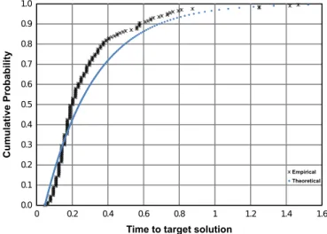
We now proceed to detailed analysis on the behavior of algorithm VNDe-ILS5p. The ﬁrst analysis is an attempt to learn more about the performance of VNDe-ILS5pif it should run on less time than 5 min. For such purpose, we make use of the time-to-target (TTT) plots proposed by Aiex et al.[1,2]. The hypothesis behind is that CPU times ﬁt a two parameter exponential distribution. Thus, for a given problem instance, TTT plots display on the ordinate axis the probability for the heuristic to obtain a solution as good as a given target value within a running time in seconds, shown on the abscissa axis. We had chosen eight instances from Table 7 to do this. For each instance we ran

Table 4

Instance Multistart-BFD BFD-VNDe VNDe-ILS5p EDP-VNDe-ILS5p LB

y.4.20.1 21 23.53 21 23.53 19 11.76 19 11.76 17

y.4.20.2 28 0.00 28 0.00 28 0.00 28 0.00 28

y.4.20.3 23 0.00 23 0.00 23 0.00 23 0.00 23

y.4.20.4 20 8.42 20 7.37 19 0.00 19 0.00 19

y.4.20.5 21 23.53 21 23.53 19 11.76 19 15.29 17

y.4.40.1 38 22.58 38 22.58 35 12.90 36 16.13 31

y.4.40.2 57 0.00 57 0.00 57 0.00 57 0.00 57

y.4.40.3 43 0.00 43 0.00 43 0.00 43 0.00 43

y.4.40.4 38 0.00 38 0.00 38 0.00 38 0.00 38

y.4.40.5 40 21.21 40 21.21 37 12.12 38 15.15 33

y.4.60.1 56 19.15 56 19.15 53 12.77 54 14.89 47

y.4.60.2 86 0.00 86 0.00 86 0.00 86 0.00 86

y.4.60.3 64 0.00 64 0.00 64 0.00 64 0.00 64

y.4.60.4 58 0.00 58 0.00 58 0.00 58 0.00 58

y.4.60.5 58 19.18 58 18.78 55 12.24 57 16.33 49

y.4.80.1 73 57.02 73 56.60 70 48.94 72 54.04 47

y.4.80.2 118 0.00 118 0.00 118 0.00 118 0.00 118

y.4.80.3 81 0.00 81 0.00 81 0.00 81 0.00 81

y.4.80.4 78 0.00 78 0.00 78 0.00 78 0.00 78

y.4.80.5 76 16.92 76 16.92 72 10.77 75 15.38 65

y.4.100.1 91 19.74 91 19.74 86 14.21 90 19.47 76

y.4.100.2 146 0.00 146 0.00 146 0.00 146 0.00 146

y.4.100.3 98 0.00 98 0.00 98 0.00 98 0.00 98

y.4.100.4 98 0.00 98 0.00 98 0.00 98 0.00 98

y.4.100.5 93 16.50 93 16.50 89 11.75 93 17.25 80

Average 9.91 9.84 6.37 7.83

Table 5

y.5.20.1 14 7.69 14 7.69 13 0.00 13 0.00 13

y.5.20.2 17 0.00 17 0.00 17 0.00 17 0.00 17

y.5.20.3 13 8.33 13 8.33 12 5.00 13 8.33 12

y.5.20.4 17 0.00 17 0.00 17 0.00 17 0.00 17

y.5.20.5 15 0.00 15 0.00 15 0.00 15 0.00 15

y.5.40.1 25 4.17 25 4.17 24 0.00 24 0.83 24

y.5.40.2 31 1.29 31 1.29 31 0.00 31 0.00 31

y.5.40.3 24 9.09 24 9.09 23 4.55 23 6.36 22

y.5.40.4 33 0.00 33 0.00 33 0.00 33 0.00 33

y.5.40.5 28 0.00 28 0.00 28 0.00 28 0.00 28

y.5.60.1 36 11.52 36 11.52 35 6.67 36 9.09 33

y.5.60.2 45 1.33 45 0.89 45 0.00 45 0.00 45

y.5.60.3 35 2.94 35 2.94 34 0.00 34 0.00 34

y.5.60.4 48 0.00 48 0.00 48 0.00 48 0.00 48

y.5.60.5 40 0.00 40 0.00 40 0.00 40 0.00 40

y.5.80.1 47 11.16 47 11.16 46 6.98 47 9.30 43

y.5.80.2 60 1.69 60 1.69 59 0.00 59 1.02 59

y.5.80.3 45 4.65 45 4.65 44 2.33 45 5.12 43

y.5.80.4 63 0.00 63 0.00 63 0.00 63 0.00 63

y.5.80.5 53 0.00 53 0.00 53 0.00 53 0.00 53

y.5.100.1 59 7.27 59 7.27 57 3.64 58 5.82 55

y.5.100.2 75 2.74 75 2.74 73 0.00 74 1.37 73

y.5.100.3 56 5.66 56 5.66 54 3.40 56 5.66 53

y.5.100.4 77 0.00 77 0.00 77 0.00 77 0.00 77

y.5.100.5 66 0.00 66 0.00 66 0.00 66 0.00 66

Average 3.18 3.16 1.30 2.12

Table 6

Comparison with multistart BFD on setZof instances.

Z.1010.20 31 17.04 31 17.04 29 7.41 30 11.11 27

Z.813.20 35 8.48 35 8.48 34 3.03 34 3.03 33

Z.617.20 46 4.55 46 4.55 44 1.36 45 2.27 44

Z.520.20 55 1.85 55 1.85 54 0.00 54 0.00 54

Z.425.20 68 3.03 68 3.03 66 0.00 67 2.12 66

Z.1010.40 59 15.69 58 14.51 55 8.63 57 12.16 51

Z.813.40 67 6.35 67 6.35 64 2.54 66 4.76 63

Z.617.40 87 4.29 87 3.57 85 1.19 86 2.38 84

Z.520.40 104 2.97 104 2.97 101 0.59 103 2.18 101

Z.425.40 129 2.70 129 2.38 127 0.79 129 2.38 126

Z.1010.60 88 14.29 87 14.03 84 9.09 87 12.99 77

Z.813.60 101 5.63 101 5.21 98 2.08 100 4.38 96

Z.617.60 133 3.91 133 3.91 129 0.78 131 2.66 128

Z.520.60 158 2.60 158 2.60 154 0.26 158 2.60 154

Z.425.60 195 2.08 195 1.98 193 0.52 197 2.71 192

Z.1010.80 116 12.62 116 12.62 112 9.51 117 13.98 103

Z.813.80 134 4.50 134 4.50 130 1.09 134 3.88 129

Z.617.80 176 3.39 176 3.27 171 0.47 175 2.57 171

Z.520.80 209 1.95 209 1.95 206 0.49 210 2.63 205

Z.425.80 261 1.56 261 1.56 258 0.47 264 2.72 257

Z.1010.100 142 13.60 142 13.60 139 11.52 146 17.44 125

Z.813.100 175 4.17 175 4.17 173 3.21 178 6.31 168

Z.617.100 222 3.06 222 3.06 220 1.85 225 4.17 216

Z.520.100 256 2.56 256 2.48 253 1.52 260 4.16 250

Z.425.100 319 2.24 318 2.18 317 1.60 325 4.42 312

(7)

VNDe-ILS5p 200 times with different seeds until the algorithm reaches the target value.Figs. 3–6show the TTT plots generated with four instances for which an average gap of 0% is reach-ed—ATT, NSF.12, y.4.20.4, y.5.100.2. For these instances we set

the target value to the optima. On the other hand,Figs. 7–10show the TTT plots generated with the instances for which a high average gap is observed—y.4.80.1, y.4.100.1, Z.1010.60,

Z.1010.80. In these cases, we set the target value to one wavelength less than the best solution found by GA-RWA. TTT plots indicate that VNDe-ILS5p is likely to obtain high quality solutions in a short time. As it can be seen, on instances tested, VNDe-ILS5p has high probability to ﬁnd very good solutions

(optimum or better than the best known) in less than 2 min, except for instance y.5.100.2, for which a little more time is needed.

The second analysis tries to bring some insight on which neighborhood brings the best gain. We performed experiments with reduced versions of VND using, along with ILS-based

Table 7

Comparison with GA-RWA on a set of difﬁcult instances.

Instance GA-RWA VNDe-ILS5p LB

l_min Gap (%) l_min Gap (%)

ATT 24 20.0 20 0.0 20

ATT2 113 0.0 113 0.0 113

Finland 46 0.4 46 0.0 46

NSF.3 22 0.9 22 0.0 22

NSF.12 39 2.6 38 0.0 38

NSF2.12 35 0.6 35 0.0 35

Z.1010.20 31 15.6 29 7.4 27

Z.617.40 87 4.0 85 1.2 84

Z.1010.60 87 13.2 84 9.1 77

Z.425.60 195 2.0 193 0.5 192

Z.1010.80 115 12.4 112 9.5 103

Z.813.80 134 3.9 130 1.1 129

Z.617.80 176 3.0 171 0.5 171

Z.520.80 209 2.0 206 0.5 205

Z.425.80 260 1.3 258 0.5 257

Z.520.100 257 2.8 253 1.5 250

y.4.20.4 20 6.3 19 0.0 19

y.3.40.5 59 12.8 56 7.4 53

y.3.60.5 86 12.5 82 7.5 77

y.4.60.5 58 18.4 55 12.2 49

y.5.60.1 36 9.7 35 6.7 33

y.3.80.1 122 15.5 115 9.3 106

y.3.80.5 113 8.8 109 4.8 104

y.4.80.1 73 55.3 70 48.9 47

y.4.80.5 75 16.0 72 10.8 65

y.5.80.1 47 11.2 46 7.0 43

y.5.80.2 60 1.7 59 0.0 59

y.4.100.1 90 18.4 86 14.2 76

y.5.100.1 58 5.5 57 3.6 55

y.5.100.2 74 1.6 73 0.0 73

Average 9.3 5.5

Fig. 3.TTT plots produced for instance ATT—target value equal to 20.

Fig. 4.TTT plots produced for instance NSF.12—target value equal to 38.

Fig. 5.TTT plots produced for instance y.4.20.4—target value equal to 19.

(8)

perturbation, neighborhoodsN1andN2separately and in

combi-nation withN3. Neighborhood N3 is not tested separately since

alone it cannot reduce the number of wavelengths.Table 8shows numerical results for the reduced versions of VND. The ﬁrst

column presents the instance. Then, the subsequent pairs of columns present the best solution and the average gap for each reduced version of VND. As before, it is reported for each proposed algorithm the results of ﬁve runs with a time limit of 5 min each. The last column presents the lower bound. We remark that although N3 alone cannot be used to improve

solutions, the reduced versions of VND using it in combination withN1orN2lead to the better results. So, a move in

neighbor-hood N3 is an important instrument to rearrange requests to

further improving moves. It is also worth noting that neighbor-hood N2 alone is not effective, but in combination with N3

becomes the most successful reduced version of VND.

Fig. 10.TTT plots produced for instance Z.1010.80—target value equal to 114.

Fig. 9.TTT plots produced for instance Z.1010.60—target value equal to 86.

Table 8

Analysis on the performance of each neighborhood.

Instance N1 N2 N1þN2 N1þN3 N2þN3 LI

lmin Gap

(%)

lmin Gap

(%)

lmin Gap

(%)

lmin Gap

(%)

lmin Gap

(%)

ATT 20 0.0 26 33.3 20 0.0 20 0.0 20 0.0 20

ATT2 113 0.0 115 2.0 113 0.0 113 0.0 113 0.0 113

Finland 46 0.0 48 5.2 46 0.0 46 0.0 46 0.0 46

NSF.3 22 0.0 22 0.0 22 0.0 22 0.0 22 0.0 22

NSF.12 38 0.0 38 0.0 38 0.0 38 0.0 38 0.0 38

NSF2.12 35 0.0 35 0.0 35 0.0 35 0.0 35 0.0 35

Z.1010.20 30 14.1 32 20.7 30 11.1 29 7.4 29 7.4 27

Z.617.40 87 3.6 88 5.5 85 2.1 86 2.4 85 1.2 84

Z.1010.60 88 14.3 89 15.8 86 12.7 85 10.4 85 10.4 77

Z.425.60 195 2.2 196 3.1 193 1.0 195 1.7 193 0.9 192

Z.1010.80 115 12.2 116 13.6 115 11.8 114 10.7 113 9.7 103

Z.813.80 134 3.9 135 5.0 132 2.9 131 1.9 131 1.6 129

Z.617.80 175 2.7 177 4.0 173 1.3 173 1.2 172 0.7 171

Z.520.80 209 2.1 210 2.8 206 0.9 207 1.4 206 0.6 205

Z.425.80 260 1.5 262 2.2 259 0.8 260 1.3 259 0.8 257

Z.520.100 256 2.5 257 3.0 254 1.9 255 2.3 254 1.7 250

y.4.20.4 19 0.0 21 11.6 19 4.2 19 0.0 19 0.0 19

y.3.40.5 58 10.9 60 14.7 58 9.4 57 7.5 57 7.5 53

y.3.60.5 85 11.4 87 13.5 84 10.1 83 8.3 83 7.8 77

y.4.60.5 58 18.4 59 21.2 58 18.4 55 13.5 55 12.2 49

y.5.60.1 36 10.9 37 14.5 36 10.3 35 6.7 35 8.5 33

y.3.80.1 121 14.5 123 17.2 119 12.8 116 10.0 116 9.6 106

y.3.80.5 113 8.7 114 10.0 111 7.5 110 5.8 109 5.4 104

y.4.80.1 73 55.7 74 58.3 73 55.3 70 49.4 70 49.4 47

y.4.80.5 75 15.7 76 17.8 75 15.4 73 12.3 72 11.7 65

y.5.80.1 47 11.2 49 14.0 47 11.2 46 7.0 46 7.9 43

y.5.80.2 59 1.4 60 2.7 59 1.0 59 0.0 59 0.0 59

y.4.100.1 90 18.9 91 20.3 90 18.7 87 14.5 87 14.5 76

y.5.100.1 58 5.5 59 8.4 58 5.5 57 3.6 57 3.6 55

y.5.100.2 74 1.4 76 4.1 74 1.4 73 0.5 73 0.5 73

(9)

5. Conclusions

We propose an algorithm for the RWA problem that alternates between a VND phase and a ILS-based perturbation phase. In the VND phase we explore three neighborhoods by trying three kinds of moves. The purpose is to reduce one wavelength. The ILS-based phase is called to introduce a perturbation in the current partition of the lightpath requests’ set. The perturbation itself does not improve a solution, but it leaves a rearrangement of lightpaths among subsets of the partition that may yield further improve-ments with another trial of VND. Even though better results were found taking BFD as constructive heuristic, VND-ILS is quite robust with respect to the initial solution and clearly outperforms a multistart variant of BFD. Computation experiments were conducted on the hardest benchmark instances, and signiﬁcant improvements upon better upper bounds from the literature were achieved. An interesting research direction is to adapt the methods to deal with possibilities of trafﬁc-grooming.

Acknowledgments

The authors wish to thank the two anonymous referees for helpful suggestions in improving this paper. The authors from Brazilian institutions were partially supported by CAPES, CNPq, and FAPEMIG, Brazil.

References

[1] Aiex RM, Resende MGC, Ribeiro CC. Probability distribution of solution time in GRASP: an experimental investigation. Journal of Heuristics 2002;8: 343–73.

[2] Aiex RM, Resende MGC, Ribeiro CC. TTT plots: a perl program to create time-to-target plots. Optimization Letters 2007;1:355–66.

[3] Banerjee D, Mukherjee B. A practical approach for routing and wavelength assignment in large wavelength-routed optical networks. IEEE Journal on Selected Areas in Communications 1996;14:903–8.

[4] Chlamtac I, Ganz A, Karmi G. Lightpath communications: an approach to high bandwidth optical WAN’s. IEEE Transactions on Communications 1992;40: 1171–82.

[5] Dutta R, Rouskas GN. A survey of virtual topology design algorithms for wavelength routed optical networks. Optical Networks Magazine 2000;1: 73–89.

[6] Hansen P, Mladenovic´ N. Variable neighborhood search. In: Glover F, Kochenberger G, editors. Handbook of metaheuristics. Kluwer; 2003. p. 145–84.

[7] Hansen P, Mladenovic´ N, Moreno Pe´rez JA. Variable neighborhood search: methods and applications. 4OR A Quarterly Journal of Operations Research 2008;6:319–60.

[8] Hansen P, Mladenovic´ N, Moreno Pe´rez JA. Variable neighbourhood search: methods and applications. Annals of Operations Research 2010;175:367–407. [9] Jaumard B, Meyer C, Thiongane B. ILP formulations for the RWA problem for symmetrical systems. In: Pardalos P, Resende M, editors. Handbook for optimization in telecommunications. Kluwer; 2006. p. 637–78.

[10] Jaumard B, Meyer C, Thiongane B. Comparison of ILP formulations for the RWA problem. Optical Switching and Networking 2007;4:157–72. [11] Jaumard B, Meyer C, Thiongane B. On column generation formulations for the

RWA problem. Discrete Applied Mathematics 2009;157:1291–308. [12] Kennington J, Olinick E, Ortynski A, Spiride G. Wavelength routing and

assignment in a survivable WDM mesh network. Operations Research 2003; 51:67–79.

[13] Krishnaswamy RM, Sivarajan KN. Algorithms for routing and wavelength assignment based on solutions of LP-relaxations. IEEE Communications Letters 2001;5:435–7.

[14] Krishnaswamy RM, Sivarajan KN. Design of logical topologies: a linear formulation for wavelength-routed optical networks with no wavelength changers. IEEE/ACM Transactions on Networking 2001;9:186–98.

[15] Lee K, Kang KC, Lee T, Park S. An optimization approach to routing and wavelength assignment in WDM all-optical mesh networks without wave-length conversion. ETRI Journal 2002;24:131–41.

[16] Lourenc-o HR, Martin OC, St ¨utzle T. Iterated local search. In: Glover P,

Kochenberger G, editors. Handbook of metaheuristics. Springer; 2003. p. 321–53.

[17] Manohar P, Manjunath D, Shevgaonkar RK. Routing and wavelengths assign-ment in optical networks from edge disjoint path algorithms. IEEE Commu-nication Letters 2002;6:211–3.

[18] Mladenovic´ N, Hansen P. Variable neighbourhood search. Computers & Operations Research 1997;24:1097–100.

[19] Mukherjee B, Banerjee D, Ramamurthy S, Mukherjee A. Some principles for designing a wide-area WDM optical network. IEEE/ACM Transactions on Networking 1996;4:684–96.

[20] Noronha T, Resende MGC, Ribeiro CC. Efﬁcient implementations of heuristics for routing and wavelength assignment. In: McGeoch CC, editor. Proceedings of the seventh international workshop on experimental algorithms. Lecture notes in computer science, vol. 5038; 2008. p. 169–80.

[21] Noronha T, Resende MGC, Ribeiro CC. A biased random-key genetic algorithm for routing and wavelength assignment. Journal of Global Optimization 2011;50(3):503–18. doi:10.1007/s10898-010-9608-7.

[22] Noronha T, Ribeiro CC. Routing and wavelength assignment by partition colouring. European Journal of Operational Research 2006;171:797–810. [23] Ramaswami R, Sivarajan KN. Routing and wavelength assignment in

all-optical networks. IEEE/ACM Transactions on Networking 1995;3:489–500. [24] Ramaswami R, Sivarajan KN. Design of logical topologies for

wavelength-routed optical networks. IEEE Journal on Selected Areas in Communications 1996;14:840–51.

[25] Skorin-Kapov N. Routing and wavelength assignment in optical networks using bin packing based algorithms. European Journal of Operational Research 2007;177:1167–79.