Financial and Real Sector Leading
Indicators of Recessions in Brazil Using
Probabilistic Models
Fernando Nascimento de Oliveira
*
Contents: 1. Introduction; 2. Data; 3. Empirical Analyses; 4. Case Studies: Forecast Indexes with Out of Sample ROC and Recessions in Brazil from 2000Q1 to 2012Q4; 5. Conclusion;
Appendix A. Tables; Appendix B. Figures.
Keywords: Recession, Forecasts, Receiver Operating Characteristic (ROC). JEL Code: E2, E27.
We examine the usefulness of various financial and real sector variables to forecast recessions in Brazil between one and eight quarters ahead. We esti-mate probabilistic models of recession and select models based on their out-of-sample forecasts, using the Receiver Operating Characteristic (ROC) function. We find that the predictive out-of-sample ability of several models vary depend-ing on the numbers of quarters ahead to forecast and on the number of regres-sors used in the model specification. The models selected seem to be relevant to give early warnings of recessions in Brazil.
Analisamos a capacidade de diversas variáveis do setor financeiro e do setor real da economia para prever recessões no Brasil entre um e oito trimestres à frente. Es-timamos modelos probabilísticos de recessão e os selecionamos com base em suas previsões fora da amostra, utilizando a funçãoReceiver Operating Characteristic (ROC). Encontramos que a capacidade preditiva fora da amostra de vários modelos variam de acordo com o número de períodos à frente que são previstos e com o nú-mero de regressores usados na especificação do modelo. Os modelos selecionados parecem ser relevantes para fornecer sinais antecipados de recessão no Brasil.
1. INTRODUCTION
The most recent financial crises showed, once again, the relevance of forecasting the downturns of business cycles. Economists in general did not anticipate the recessions that took place worldwide.
Economies evolve over time and are subject, sometimes, to large unanticipated structural breaks. Such breaks can be precipitated by sudden changes in economic policy, major scientific and technological discoveries and innovations, political turmoil or permanent macroeconomic shocks.
Economists often use complex mathematical models to forecast the path of the GDP and the like-lihood of a recession (Bank of England,2000;Hatch,2001). The models used to understand and forecast processes as complicated as GDP are far from perfect representations of their behavior.1
Simpler indicators such as interest rates, spread of interest rates, stock price indexes, monetary aggregates, and some readily available real sector indicators contain very relevant information about future economic activity.2
These indicators can be used to verify both econometric and judgmental predictions by signaling a problem that might otherwise have gone unidentified. If forecasts from an econometric model and forecasts from these indicators agree, confidence in the model’s results can be enhanced. In contrast, if these indicators forecasts give a different signal, it may be worthwhile to review the assumptions and relationships that led to the prediction of the more complex econometric models.
The indicators mentioned above are, in general, associated with expectations regarding the occur-rence of future events, as shown byEstrella & Mishkin(1997) andStock & Watson(2001), and therefore are natural candidates for leading indicators of economic activity. They also present some of the neces-sary properties of leading indicators. They conform to the business cycles; have economic significance, statistical accuracy and little need for revisions. Therefore, the development, as well as the monitor-ing, of such indicators can be very relevant for the formulation and implementation of macroeconomic policies, given that they give additional evidence about the state of the economy.
In this paper, we examine the usefulness of various financial and real sector variables in out-of-sample predictions of whether or not the Brazilian economy will be in a recession between one and eight quarters in the future. Variables with potential predictive content are selected from a broad array of candidates and are examined by themselves and in some plausible and parsimonious combinations.
We focus simply on predicting recessions rather than on quantitative measures of future economic activity. We believe that this is a useful exercise because it addresses a question frequently posed by policy makers and market participants.3
We also are not concerned with misspecified models. AsHendry & Clements(2002) posit, it is by now well documented in the literature the fact that well specified models based on historical data may forecast out-of-sample worse than misspecified ones. The fundamental reason for this is the existence of unanticipated shifts or structural breaks in the economy in the future.4 After such a shift, a
previ-ously well-specified model may forecast less accurately than one that is misspecified. The best causal description of the economy may not be robust to such sudden shifts.5
To assess how well each indicator variable predicts recessions, we use the so-called extreme value model—a particular case of a probabilistic model—, which, in our applications, directly relates the probability of being in a recession to specific groups of explanatory variables.6
We also assess the capacity of variables to forecast recessions, and by this contribute to the lit-erature, by selecting models based on out-of-sample forecasts, using a metric related to the Receiver
1There is a known lag in GDP series all over the world. In addition, GDP series receives several revisions as time goes by. So we may interpret our exercise as one in which our projections may be understood as nowcasts or even backcasts.
2SeeEstrella & Mishkin(1997) for a discussion.
3Hamilton(1989) states that it makes sense to think of the economy as evolving differently within distinct discrete states.
4Hansen(2001),Stock & Watson(1996),Koop & Potter(2000) are interesting discussions about the limitations of forecasting in the
presence of structural breaks.
5AsHendry & Clements(2002) stress the distributions of future outcomes are not the same as those in sample. That means that
well specified in-sample models will not necessarily forecast out-of-sample better than badly specified in-sample models. It may also be the case that variables that seem irrelevant will forecast better than relevant ones. In addition, further ahead interval forecasts generally lead to worst forecasts than near-horizon ones. All these facts seem highly damaging to the forecasting endeavor.
Operating Characteristic (ROC) curve.7 The ROC curve plots the fraction of true positives (crisis
=1) that a given model signals (out of all positives in the sample) vs. the fraction of false positive signals (out of all negatives in the sample) along contiguous threshold settings. The best model according to this criterion is the one that delivers the highest trade-off frontier between true and false alarms.8,9
We find that the predictive out-of-sample ability of several models vary depending on the numbers of quarters ahead to forecast and on the number of regressors used in the model specification. The best models selected can be thought as early warning signals of recessions in Brazil. Our selected models do good job in anticipating this recession.
There is a vast literature by now that search for good leading indicators of recessions such as we do in this paper. Just to mention some,Estrella & Mishkin(1997) use a probit model to evaluate the usefulness of financial variables to predict U.S. recessions, both in- and out-of-sample. Their full sample covers a number of recessions. Their main findings are that stock prices are the best leading indicators of recessions at the 1- and 2-quarter horizons.
Bernard & Gerlach(1996) examine the ability of the term structure to predict recessions in eight
countries (Belgium, Canada, France, Germany, Japan, the Netherlands, the United Kingdom and the United States) between the period 1972:1 and 1993:4. For all the countries, their study also shows that the yield curve provides information about the likelihood of future recessions up to eight quarters ahead.
Lamy (1997) studies several macroeconomic indicators, to verify if they predict recessions in Canada. He finds the Department of Finance index of leading indicators of economic activity and the Bank of Canada nominal monetary conditions index to be strongest at predicting recessions for a fore-cast horizon of one quarter. At the horizon of two to four quarters, he finds the yield curve to be the best variable to predict recession.
In the case of forecasting recessions in Brazil, we can select two very interesting papers in the literature. Morais & Chauvet(2011) build leading indicators to predict the capital goods business cycle in Brazil. They propose a probit model with autoregressive dynamics. Their results indicate that the dynamic probit model has a better forecasting performance than the simple probit model in several aspects, both in and out of sample.
Another empirical paper for Brazil isDuarte, Issler, & Spacov(2004). The authors build several coincident and leading indicators of economic activity in Brazil to forecast recessions. Their results show that the best indicators for this purpose are the ones that follow the methodology of the Conference Board.
Two forecasting results emerge from our study. First and most important, the criteria to select models for forecast should be always out-of-sample performance. AsHendry & Clements(2002) point out the distributions of future outcomes are not the same as those in sample. That means that well specified in sample models will not necessarily forecast out-of-sample better than badly specified in-sample models. It may also be the case that variables that seem irrelevant will forecast better than relevant ones. Second, it is important to determine the optimal out-of-sample horizon for each forecast-ing model. Further ahead interval forecasts generally lead to worst forecasts than near-horizon ones.
Our results also confirm that despite its non-specific assumptions, a theory of forecasting which allows for structural breaks may provide a useful basis for interpreting, and circumventing, systematic forecast failure in economics.
7The Receiver Operating Characteristic (ROC), or simply ROC curve, is commonly used in signal detection theory. It is a graphical plot, which describes the performance of a binary classifier system as its discrimination threshold is varied. It is built by plotting the fraction of true positives out of the total actual positives (TPR=true positive rate) vs. the fraction of false positives out of
the total actual negatives (FPR=false positive rate), at various threshold settings. ROC analysis is related in a direct and natural
way to cost/benefit analysis of diagnostic decision making.
8We define the model ROC as the value of the integral of the ROC function of the model from0to1.
The rest of the paper is organized as following. Section 2describes the data. Section 3presents the empirical analysis.Section 4presents some case studies analyses.Section 5concludes.
2. DATA
The macroeconomic indicators have a good performance record in predicting real activity. The financial series we look at may be less prone to the over fitting problem than the traditional macroeconomic indicators.
Another important consideration is the possible lag in the availability of the data for the explana-tory variables. Some variables, such as interest rates and stock prices, are available on a continuous basis with no informational lag. In contrast, many monthly macroeconomic series are only available one or two months after the period covered by the data, and GDP has a lag of almost one full quarter.
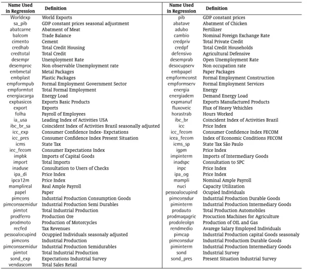
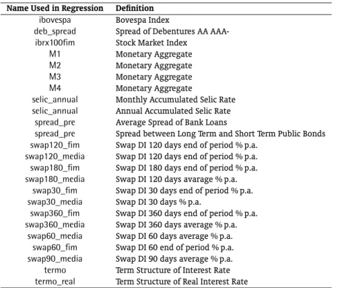
Our sample has quarterly data and goes from the first quarter of 1991 to the fourth quarter of 2015.Table A-1(see sectionA.1inAppendix A) shows all the names of all the real sector variables we use in our empirical exercise. We have 83 real sector variables. We use the level and the first difference in logarithm of the series variables. When possible, we also use the seasonally adjusted series in level or in the first difference in logarithm.10Table A-2shows the financial sector variables. We have 24 variables.
Once more, we use the level as well as the first difference in logarithm of these series.
The recession variable is built using the standard two consecutive quarters of negative variation of GDP with seasonal adjustment. We have 8 quarters of recession, which are: 1999Q1, 2001Q3, 2003Q2 and 2009Q1, 2014Q2, 2015Q2, 2015Q3, 2015Q4.11
3. EMPIRICAL ANALYSES
3.1. Forecasting Methodology
We now turn to the question of how to choose the models that best forecast out-of-sample recessions. Model misspecification by itself cannot account for forecast failure: in the absence of changed economic conditions, a model’s out-of-sample forecast performance would, on average, be the same as its in sam-ple fit to the data.
If forecast failure is primarily due to forecast-period location shifts asHendry & Clements(2002) stress, then there are no possible within sample tests of the models. Structural breaks happen all the time in the economy. Therefore, choosing models to forecast based on in sample forecast performance seems to be a great mistake.
To address these issues we utilize measures out-of-sample performance to discriminate between the best forecast models. We decided not to use Mean Squared Errors (MSE) or any of its variants as our main criteria to select models. The growing consensus among researchers who have been making com-parisons among forecasting methods is that the MSE should not be used.Newbold(1993), for example, explores the deficiencies of mean squared errors as a performance measure.
Thompson(1990) also concluded that MSE is not appropriate. He proposed a variation on the
MSE, the log mean squared error ratio (LRM), that would be appropriate for making comparisons across series. The LMR takes the log of the ratio calculated by dividing the proposed model’s MSE by the MSE of a benchmark model.
The out sample performance of our models is gauged with the so-called ROC curve as a model selection tool. The ROC curve plots the fraction of true positives (crisis=1) that a given model signals
10In the case of the first difference in logarithm, we append the series name with “dlog”. In the case of seasonality, we append the series name with “sa_”.
(out of all positives in the sample) vs. the fraction of false positive signals (out of all negatives in the sample) along contiguous threshold settings. The best model according to this criterion is the one that delivers the highest trade-off frontier between true and false alarms. Such a choice will be guided by the relative cost of failing to predict a crisis vs. that of a false alarm, credibility cost.
A clear advantage of this approach over traditional model selection criteria previously used in the forecast literature is that the analyst does not have to take a stand a priori on which region of the trade-off to pick. Distinct models deliver a distinct ROC curve and the overall “best” is the one that delivers the highest area under the curve, i.e., the higher outward frontier above the 45-degree line, where the latter traces out the good vs. false positive trade-off under random guesses.
There are other several advantages of ROC in comparison to other possible metrics of forecasting comparisons. For example,Estrella & Mishkin(1997) use out-of-sample PseudoR2as a metric to compare
the performance of models. As the authors acknowledge, in some cases out-of-sample PseudoR2furnish
negative results. This makes it a much worse metric than ROC in our view to compare the out-of-sample performance of models.12
The ROC methodology focuses on a fundamental characteristic of forecasting, that is, its ability to capture the occurrence of an event with an underlying high hit rate, while maintaining the false alarm rate to some acceptable level.
Recent applications of the ROC curve methodology to historical data on domestic bank credit in 14 advanced countries are provided inJordà, Schularick, & Taylor(2011), whereasSatchell & Xia(2006) present an earlier application to credit rating models.Catão & Milesi-Ferretti(2013) use it in an in-sample framework to forecast financial crisis. Yet, we are not aware of any other paper that uses it in the same way and context that we do in this paper.13
ROC, as any other empirical methodology, has also some drawbacks. As it is only based on a forecast of binary values, it ignores the magnitude of the forecast errors. It may have low power in small samples, because it does not consider the magnitudes of these forecast errors. ROC can be understood as a criteria of unconditional evaluation, because it does not make a distinction between the existence (or not) of temporal clusters of the binary variable (Kupiec,1995;Christoffersen,1998). Finally, although very useful to establish a forecast ranking among different models, one cannot verify if two models produce forecasts that are statistically significant and different.
To address some of the issues mentioned above, we will compare our results with some more traditional forecast models of rare events, such as the directional tests ofPesaran & Timmermann(1992).
We are interested in selecting one to four regressors models that best forecast recessions in Brazil from 1 to 8 quarters ahead.14 Being more specific, our methodology is the following. We estimate an
equation such as (1) below using a probabilistic extreme value model with only one regressor.
Pr(Yt+K =1 Xt
)
=f(Xt), (1)
wheref(
Xt) =exp(
−exp(−Xβ))(extreme value function), andK=1, . . . ,8.
Our first estimation period goes from 1991Q1 to 2002Q1. Then we forecastKperiods ahead (K from1to8), considering levels of cutoff probabilities that range from0.005to1and that vary in each
step by0.005. If the forecast value of recession is less that the cutoff probability that we are considering
12Lahiri & Wang(2013) stress that often-conventional goodness-of-fit statistics in probabilistic models, such as PseudoR2, among
others fail to identify the type of I and type of II errors in predicting the event of interest. Lahiri and Wang examine the quality of probability forecasts in terms of calibration, resolution and alternative variance decompositions. They discuss several measures of goodness of fit, like, for instance, the Brier’s Quadratic Probability Score, the Prequential Test for Calibration, the Skill Score and the Murph and Yates Decompositions.
13SeeCatão & Milesi-Ferretti(2013) for a utilization of ROC to forecast financial crisis.
we take the forecast to be zero. Otherwise, the forecast is one. We compare these values with the values of the recessions that occurred after the estimation period.15
We then increase the estimation period by one quarter and repeat the process above for every forecast period until we reach our final estimation period that goes from 1991Q1 to 2015Q3. We then calculate the number of success (correct forecasts) divided by the total number of successes (recessions); we also calculate the number of failures (false positive signals) and divide that by the total number of failures (all periods in which there were no recessions). By doing this, we are able to build a ROC function for each model with one regressor for everyKquarters ahead forecast. We then integrate this function from0to1and name this value the ROC of the model. The best models are the one with the highest ROCs for eachK forecast period.
We use the regressors of the models selected with one regressor in the specifications of the models with two regressors. We repeat the methodology above for every one of these models and select the best models as the ones with the highest ROCs for everyKforecast period. After selecting the two-regressor models, we repeat the process with three regressors, where two of them are the ones that proved best in forecasting. Finally, we choose the four-regressor models using the same process and considering the three regressor models selected as the basis for the four-regressor models.
3.2. Results
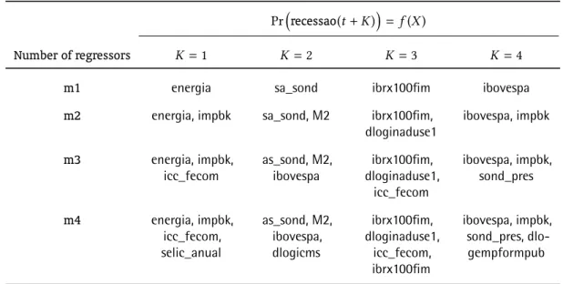
Table A-3andTable A-4(see sectionA.2inAppendix A) present the best models in terms of one-year
ahead forecasts. Table A-5presents the variables that make the models andTable A-6present the ROC values of these models. For one-quarter ahead forecasts, with one regressor the best model is the one that hasenergiaas the only regressor. The out-of-sample ROC of this model is 0.8710. In the case of the forecasts of two quarters, with one regressor the best model is the one that hassa_sondas the only regressor. The out-of-sample ROC of this model is 0.5701. When we consider 3 quarters ahead forecasts, with three regressors the best model is the one that hasicc_fecom,ibrx100fimanddloginaduse1. The ROC of this model is 0.9777. Finally, for 4 quarters ahead the best model is the four regressor model
withimpbk,sond_pres,ibovespaanddlogempformpubwith ROC of 0.9990.
For forecasts of more than one year, the results are presented inTable A-5and Table A-6(see sectionA.2inAppendix A).Table A-5presents the variables that make the models andTable A-6present the ROC values of these models. For five periods ahead, the best model is the one that has four regressors,
ibovespa,sond_press,empformtotanddlogprodauto, with ROC of 0.9732. For six quarters ahead, the
best model is the one with three regressorsicc_fecom,balcom,empformpubwith ROC of 0.9800. For seven quarters ahead, the best model is the one with 3 regressors,M2,dlogibovespa,dlogimpbk, and ROC of 0.6672. Finally, for eight quarters ahead the best model is the one with 3 regressors,icc_fecom, impbk,energia, with ROC of 0.9405.
We use the maximum variance ofBirnbaum & Klose(1957) and verify that all ROC areas presented in tablesA-3toA-6are statistically significant. As one can observe from the results, financial variables are relevant for forecasting. Particularly, those related to the stock market, likeibovespaandibrx100fim. These variables take part as regressors in many specifications. They are observed individually over their respective primary horizons, or they may be combined to produce very accurate models in terms of out of sample forecasts.
In general, prices of financial assets are supposed to contain expectations about the future path of the economy. The most convincing theoretical foundation of this assumption is the expectations theory of the term structure. The expectations hypothesis postulates that, for any choice of holding period, investors do not expect to realize different returns from holding bonds or bills of different maturities.
Not consistent with the findings ofEstrella & Mishkin(1997),Estrella & Hardouvelis(1990),Bernard
& Gerlach(1996), andPlosser & Rouwenhorst(1994), we have not shown that the term spread has
sig-nificant information content for forecasting recessions in Brazil. The term structure of interest rate is an important leading indicator for recessions in USA.
Some real sector indicators seem also relevant to forecast. The series energia, empformtot and empformpub are the ones that are more important. Their appearance in the best models is expected, because they reflect earlier than other real sector variables the possibility of a recession in the near future.
Confidence indicators and some monetary aggregates also play special roles in forecasting. In the case, of confidence indicators, we ponder that this may occur because households are getting better in understanding the dynamics of business cycles. In the case of monetary aggregates, we think the reason may be related to the high demand for public bonds in Brazil.
In sample results are based on equations estimated over the entire sample period. Their predic-tions or fitted values are then compared with the actual recession dates. Three types of results are presented: an in-sample ROC, a PseudoR2, and a MSE. We present the statistics of the same models
we selected from the out sample forecasts analysis above in TablesA-7andA-8(see sectionA.3in
Ap-pendix A). The in sample forecasts measures give a different indication of the forecast capacity of the
models selected. Some models that have better out-of-sample performance, do worse if we consider in-sample measures. Again, using theBirnbaum & Klose(1957) statistic we verify that all ROC values are statistically significant.
InTable A-9andTable A-10(see sectionA.4inAppendix A), we present thePesaran & Timmermann
(1992) statistic of the directional tests, which gives an idea of how well our models selected are good in forecasting change in direction of the variable of interest and the MSE statistic associated with each one of the models. Only a few of the statistics are not statistically significant (those in boldface). The results show clearly that the great majority of the models selected with the ROC criteria reject the null Hypothesis of not being able to forecast the changes in directions.
4. CASE STUDIES: FORECAST INDEXES WITH OUT OF SAMPLE ROC AND RECESSIONS IN
BRAZIL FROM 2000Q1 TO 2012Q4
Predicting the future is a tricky business. A good example of what may happen is provided by the experience with theStock & Watson(1990) leading indicators. Stock & Watson (1993) describe and analyze the disappointing performance of their indicator predicting the 1990–1991 recession.
Here we examine the performance of our chosen forecast models to predict recessions in Brazil in the period from 2000Q1 to 2015Q4. We consider the eight models that gave us the best out-of-sample ROC for each forecast period. We construct 4 indexes. The first one (Index1) is an equal weighted average of the forecasts of our best models in terms of ROC for each forecast horizon, from one to eight quarters. The second one (Index2) is a weighted average of our best forecast models (the one quarter ahead forecast with weight equal to eight and the others with weights decreasing until one). The third one (Index3) is an equal weighted average of the best ROC models selected (one to four regressors) for all horizons. The fourth indicator is a weighted weighted average of our best forecast models (the one quarter ahead forecast with weight equal to four and the others with weights decreasing until one).
Our comparison analyses are graphical and are of three types. We look at how these series behaved individually to forecast the recessions. We compare our forecasts with those made by a leading financial indicator of GDP that we built. Finally, we look at how our forecasts compare with those made by the market and for this we use the GERIN database of GDP forecasts in Brazil the market.
in all recession quarters. This seems to be evidence that they are anticipating recessions. They seem relevant as warnings of recessions.
We also build a leading financial indicator index based on Index of Economic Activity, Brazil (IBC-Br), that incorporates the pathway of the variables considered as proxies to the development of three most important economy sectors (agriculture and livestock, industry, and services).
To build the index, we considered the same 24 financial series we used in this paper. Initially, we calculated the current and lagged correlations between these series and the first difference of IBC-BR seasonally adjusted. Then, these series were submitted to Granger causality tests to find the final selection: end of period monthly return of ibovespa ibrx100fim lagged 2 periods. Figure B-4presents the dynamics of this index together with the average of the indexes we built with ROC. The figure shows that our recession indicators do a better job in forecasting recession in all cases.
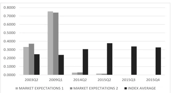
Finally, we compare our forecasts with the market forecasts. The Central Bank of Brazil collects every week forecasts of market participants with respect to five or four quarters ahead in time of GDP growth in Brazil. We create a market signal variable of recession if the market forecasts two consecutive quarters of negative growth. Otherwise, this variable is zero. Then we take the quarterly average of this variable. We create two market signals, one is an equally weighted average of the quarterly forecasts and the other is a weighted forecast (the one quarter ahead forecast with weight equal to four and the others with weights decreasing until one). Figure B-5shows the market signal are slightly better in predicting the 2003Q2 and 2009Q1 recessions but that our indicators are much better in predicting the more recent recessions, 2014Q2 and 2015Q2, 2015Q3.
5. CONCLUSION
Economic forecasting that allows for structural breaks and misspecified models has radically different implications from one that considers stationary and well-specified ones. It is well known by now in the literature that models that are well specified in- sample may perform very poorly out sample. There are many reasons for this, but maybe the most important is the occurrence of structural breaks in out-of-sample.
In this paper, we examine the usefulness of various financial and real sector variables in out-of-sample predictions of whether or not the Brazilian economy will be in a recession between one and eight quarters in the future. Variables with potential predictive content are selected from a broad array of candidates and are examined by themselves and in some plausible combinations.
The models selected, in our view, adapt quickly after any shift is discovered, therefore avoiding systematic failure of forecasting. We think they capture some of the robustness characteristics of the models that win forecasting competitions.
The predictive out-of-sample capacity of several models vary depending on the numbers of quar-ters ahead to forecast and on the number of regressors used in the model specification.
We think that our results are relevant for the literature of forecasting rare events, such as reces-sions. The best models selected can be thought as early warning signals of recessions in Brazil.
Of course, we do not propose that these indicators substitute macroeconomic models and judg-mental forecasts. Rather, we conclude that our selected models can usefully supplement the former models and other forecasts, and can serve as a quick, reliable check of more elaborate predictions.
REFERENCES
Bernard, H., & Gerlach, S. (1996, September). Does the term structure predict recessions? The international evidence(Working Paper No. 37). Basel, Switzerland: Bank for International Settlements. Retrieved from http://www.bis.org/publ/work37.htm
Birnbaum, Z. W., & Klose, O. M. (1957). Bounds for the variance of the Mann–Whitney statistic. Annals of Mathematical Statistics,28(4), 933–945.
Catão, L. A. V., & Milesi-Ferretti, G. M. (2013, May).External liabilities and crises(IMF Working Paper No. WP/13/113). International Monetary Fund. Retrieved fromhttp://www.imf.org/external/pubs/cat/longres.aspx?sk= 40545.0
Christoffersen, P. F. (1998). Evaluating interval forecasts.International Economic Review,39(4), 841–862. Retrieved fromhttp://www.jstor.org/stable/2527341
Duarte, A. J. M., Issler, J. V., & Spacov, A. (2004). Indicadores coincidentes de atividade econômica e uma cronologia de recessões para o Brasil.Pesquisa e Planejamento Econômico,34(1), 1–37. Retrieved fromhttp://ppe.ipea .gov.br/index.php/ppe/article/view/62
Estrella, A., & Hardouvelis, G. (1990). Possible roles of the yield curve in monetary policy. In Federal Reserve Bank of New York (Ed.),Intermediate targets and indicators for monetary policy(pp. 339–362). New York, NY: Federal Reserve Bank of New York. Retrieved fromhttps://fraser.stlouisfed.org/docs/publications/books/ frbny_itimp.pdf
Estrella, A., & Mishkin, F. S. (1997). The predictive power of the term structure of interest rates in Europe and the United states: Implications for the European Central Bank.European Economic Review,41(7), 1375–1401. doi:10.1016/S0014-2921(96)00050-5
Hamilton, J. D. (1989). A new approach to the economic analysis of nonstationary time series and the business cycle.Econometrica,57(2), 357–384. Retrieved fromhttp://www.jstor.org/stable/1912559
Hansen, B. E. (2001). The new econometrics of structural change: Dating breaks in U.S. labour productivity.Journal of Economic Perspectives,15(4), 117–128. doi:10.1257/jep.15.4.117
Hatch, N. (2001). Modeling and forecasting at the Bank of England. In D. F. Hendry & N. R. Ericsson (Eds.), Under-standing economic forecasts(pp. 124–148). Cambridge, MA: MIT Press.
Hendry, D. F., & Clements, M. P. (2002, August). Economic Forecasting: Some Lessons from Recent Research
(Royal Economic Society Annual Conference 2002 No. 99). Royal Economic Society. Retrieved fromhttps:// ideas.repec.org/p/ecj/ac2002/99.html
Jordà, Ò., Schularick, M., & Taylor, M. A. (2011). Financial crises, credit booms, and external imbalances: 140 years of lessons.IMF Economic Review,59(2), 340–378. doi:10.1057/imfer.2011.8
Koop, G., & Potter, S. (2000). Nonlinearity, structural breaks, or outliers in economic time series. In W. A. Barret, D. F. Hendry, S. Hylleberg, T. Teräsvirta, D. Tjøstheim, & A. Würtz (Eds.),Nonlinear econometric modeling in time series analysis: Proceedings of the Eleventh International Symposium in Economic Theory(pp. 61–78). Cambridge University Press.
Kupiec, P. H. (1995). Techniques for verifying the accuracy of risk measurement models.The Journal of Derivatives,
3(2), 73–84. doi:10.3905/jod.1995.407942
Lahiri, K., & Wang, J. G. (2013). Evaluating probability forecasts for GDP declines using alternative methodologies.
International Journal of Forecasting,29(1), 175–190. doi:10.1016/j.ijforecast.2012.07.004
Lamy, R. (1997). Forecasting Canadian recessions with macroeconomic indicators(Working Paper No. 97-03). Ottawa: Department of Finance Canada.
Mitchell, W. C., & Burns, A. F. (1961). Statistical indicators of cyclical revivals. In G. H. Moore (Ed.),Business cycle indicators, volume 1(pp. 162–183). Princeton University Press. Retrieved fromhttp://www.nber.org/ chapters/c0726
Moore, G. H. (1961). Statistical indicators of cyclical revivals and recessions. In G. H. Moore (Ed.),Business cycle indicators, volume 1(pp. 184–260). Princeton University Press. Retrieved fromhttp://www.nber.org/ chapters/c0727
Morais, A. C., & Chauvet, M. (2011). Leading indicators for the capital goods industry. Brazilian Review of Econometrics,31(1), 137–171. doi:10.12660/bre.v31n12011.3630
Newbold, P. (1993). On the limitations of comparing mean square forecast errors: Comment.Journal of Forecasting,
12(8), 658–660. doi:10.1002/for.3980120811
Pesaran, M. H., & Timmermann, A. (1992). A simple nonparametric test of predictive performance. Journal of Business & Economic Statistics,10(4), 461–465. doi:10.1080/07350015.1992.10509922
Pesaran, M. H., & Timmermann, A. (2009). Testing dependence among serially correlated multicategory variables.
Journal of the American Statistical Association,104(485), 325–337. doi:10.1198/jasa.2009.0113
Plosser, C. I., & Rouwenhorst, K. G. (1994). International term structures and real economic growth. Journal of Monetary Economics,33(1), 133–155. doi:10.1016/0304-3932(94)90017-5
Satchell, S., & Xia, W. (2006, August). Analytic models of the ROC curve: Applications to credit rating model validation(Research Paper No. 181). Sydney: University of Technology Sydney – Quantitative Finance Research Center. Retrieved fromhttp://www.qfrc.uts.edu.au/research/research_papers/rp181.pdf Stock, J. H., & Watson, M. W. (1990, April).New indexes of coincident and leading economic indicators(Working
Paper No. 1380). National Bureau of Economic Research (NBER). Retrieved fromhttp://www.nber.org/papers/ r1380
Stock, J. H., & Watson, M. W. (1993). A procedure for predicting recessions with leading indicators: Economet-ric issues and recent experience. In J. H. Stock & M. W. Watson (Eds.),Business cycles, indicators, and forecasting(pp. 95–156). The University of Chicago Press.
Stock, J. H., & Watson, M. W. (1996). Evidence on structural instability in macroeconomic time series relations.
Journal of Business & Economic Statistics,14(1), 11–30. doi:10.1080/07350015.1996.10524626
Stock, J. H., & Watson, M. W. (2001, March).Forecasting output and inflation: The role of asset prices(Working Paper No. 8180). National Bureau of Economic Research (NBER). doi:10.3386/w8180
APPENDIX A. TABLES
A.1. Descriptive Analysis of the Database
Our sample has quarterly data and goes from the first quarter of 1991 to the fourth quarter of 2015. We have 84 real sector variables. Table A-1shows the real sector variables. We use the level and the first difference in logarithm of the series variables. When possible, we also use the seasonally adjusted series in level or in the first difference in logarithm. Table A-2shows the financial sector variables. We have 26 variables. Once more, we use the level as well as the first difference in logarithm of these series.
Table A-1.Real sector variables.
Name Used
in Regression Definition in RegressionName Used Definition
Worldexp World Exports pib GDP constant prices
sa_pib GDP constant prices seasonal adjustment abatave Abatment of Chicken
abatcarne Abatment of Meat adubo Fertilizer
balcom Trade Balance cambio Nominal Foreign Exchange Rate
cimento Cement credpriv Total Private Credit
credhab Total Credit Housing credpf Total Credit Households credtotal Total Credit defensivo Agricultural Defensive desempr Unenployment Rate desemprab Open Unemployment Rate desemproc Non observable Unemployment rate desocupserv Non occupation rate
embmetal Metal Packages embpapel Paper Packages
embplast Plastic Packages empformconst Formal Employment Construction empformpub Formal Employment Government Sector empformserv Formal Employment Services
empformtot Total Formal Employment energia Energy
energiacarga Energy Load energiadem Demand Energy Load expbasicos Exports Basic Products expmanuf Exports Manufactured Products
export Exports fluxoveic Flux of Heavy Vehichles
folha Payroll of Employees horastrab Hours Worked
ia_usa Leading Index of Activities USA ibc_br Coincident Index of Activities Brazil ibc_br_sa Coincident Index of Activities Brazil seasonally adjusted icc Price Index
icc_exp Consumer Confidence Index- Expctations icc_fecom Consumer Confidence Index FECOM icc_pres Consumer Confidence Index Present Situation icea_fecom Index of Economic Conditions FECOM
icms State Tax icms_sp State Tax São Paulo
iec_fecom Consumer Expectations Index igpm Price Index
impbk Imports of Capital Goods impinterm Imports of Intermediary Goods
import Total Imports inadspc Consultation to SPC
inaduse Consultation to Users of Checks inpc Price Index
ipa_di Price Index ipa_og Price Index
ipca12m Price Index mampli Nominal Ample Payroll
mamplireal Real Ample Payroll nuci Capacity Utilization
papel Paper pessoalocupind Ocupied Individuals
pimcons Industrial Production Consumption Goods pimconsdur Industrial Production Durable Goods pimconssemidur Industrial Production Semi Durables piminterm Industrial Production Intermediary Goods
pimtot Total Industrial Production prodauto Total Production Automobiles prodferro Production Ore prodmaqagric Procuction Machines for Agriculture prodmoto Production of Motorcycles prodoleolgn Production of OIL and Gas
recfed Tax Revenues rendmedio Avarege Salary Employed Individuals pessoalocupind Ocuppied Individuals seasonaly adjusted pimcap Industrial Production capital Goods seasonaly
pimcons Industrial Production pimconsdur Industrial Productiom Durable Goods pimconssemidur Industrial Production Semidurables piminterm Industrial Production Intermediary Goods
pimtot Total Industrial Production sond Industrial Survey
Table A-2.Financial sector variables.
Name Used in Regression Definition
ibovespa Bovespa Index
deb_spread Spread of Debentures AA
AAA-ibrx100fim Stock Market Index
M1 Monetary Aggregate
M2 Monetary Aggregate
M3 Monetary Aggregate
M4 Monetary Aggregate
selic_annual Monthly Accumulated Selic Rate
selic_annual Annual Accumulated Selic Rate
spread_pre Average Spread of Bank Loans
spread_pre Spread between Long Term and Short Term Public Bonds
swap120_fim Swap DI 120 days end of period % p.a.
swap120_media Swap DI 120 days end of period % p.a.
swap180_fim Swap DI 180 days end of period % p.a.
swap180_media Swap DI 120 days avarage % p.a.
swap30_fim Swap DI 30 days end of period % p.a.
swap30_media Swap DI 30 days % p.a.
swap360_fim Swap DI 360 days end of period % p.a.
swap360_media Swap DI 360 days average % p.a.
swap60_media Swap DI 60 days average % p.a.
swap60_fim Swap DI 60 end of period % p.a.
swap90_media Swap DI 90 days average % p.a.
termo Term Structure of Interest Rate
termo_real Term Structure of Real Interest Rate
A.2. Out-of-sample ROCs
Our sample has quarterly data and goes from the first quarter of 1991 to the fourth quarter of 2015. Our leading indicators of recessions are composed of 83 real sector variables and 24 financial variables. We use both levels and first difference of these variables seasonaly adjusted and non seasonaly adjusted. We use a probabilistic extreme value model with only one regressor.
Our first estimation period goes from 1991Q1 to 2002Q1. Then we forecastKperiods ahead (K from 1 to 8), considering levels of cutoff probabilities that range from 0.005 to 1 and that vary in each step by 0.005. If the forecast value of recession is less that the cutoff probability that we are considering we take the forecast to be zero. Otherwise, the forecast is one. We compare these values with the values of the recessions that occurred after the estimation period. We then increase the estimation period by one quarter and repeat the process above for every forecast period until we reach our final estimation period that goes from 1991Q1 to 2015Q3. We then calculate the number of success (correct forecasts) divided by the total number of successes (recessions); we also calculate the number of failures (false positive signals) and divide that by the total number of failures (all periods in which there were no recessions). By doing this we are able to build a ROC function for each model with one regressor for everyK quarters ahead forecast. We then integrate this function from 0 to 1 and name this value the ROC of the model.
Finally, we choose the four regressor models using the same process and considering the three regressor models selected as the basis for the four regressor models. Table A-3shows the one year ahead models with the best forecasts andTable A-4shows their ROCs. Table A-5shows the two-year best models andTable A-6shows their ROCs.
Table A-3.Models of one year ahead forecasts.
Pr(recessao(t+K))=f(X)
Number of regressors K=1 K=2 K=3 K=4
m1 energia sa_sond ibrx100fim ibovespa
m2 energia, impbk sa_sond, M2 ibrx100fim,
dloginaduse1
ibovespa, impbk
m3 energia, impbk,
icc_fecom
as_sond, M2, ibovespa
ibrx100fim, dloginaduse1,
icc_fecom
ibovespa, impbk, sond_pres
m4 energia, impbk,
icc_fecom, selic_anual
as_sond, M2, ibovespa, dlogicms
ibrx100fim, dloginaduse1,
icc_fecom, ibrx100fim
ibovespa, impbk, sond_pres, dlo-gempformpub
Table A-4.ROCs of one year ahead models.
Pr(recessao(t+K))=f(X)
Number of regressors K=1 K=2 K=3 K=4
m1 0.8710 0.5701 0.6637 0.6885
m2 0.5413 0.7070 0.7402 0.4497
m3 0.8878 0.8823 0.9443 0.9912
Table A-5.Models two years ahead forecast.
Pr(recessao(t+K))=f(X)
Number of regressors K=5 K=6 K=7 K=8
m1 ibovespa icc_fecom M2 icc_fecom
m2 ibovespa,
sond_pres
icc_fecom, balcom
M2, dlogibovespa
icc_fecom, impbk
m3 ibovespa,
sond_pres, empformtot
icc_fecom, balcom, empformpub
M2, dlogbovespa,
desemp
icc_fecom, impbk, energia
m4 ibovespa,
sond_pres, empformtot, dlogprodauto
icc_fecom, balcom, empformpub,
dlogimpbk
M2, dlogbovespa,
desemp, ibovespa
icc_fecom, impbk, energia,
expmanuf
Table A-6.ROCs of one year ahead models.
Pr(recessao(t+K))=f(X)
Number of regressors K=5 K=6 K=7 K=8
m1 0.5098 0.6476 0.5421 0.9571
m2 0.6672 0.4771 0.4682 0.4095
m3 0.9147 0.9800 0.8569 0.9405
A.3. In-sample forecasts statistics
Our sample has quarterly data and goes from the first quarter of 1991 to the fourth quarter of 2015. Our leading indicators of recessions are composed of 83 real sector variables and 24 financial variables. We present insample ROC, PseudoR2 and MAE of the models selected with out-of-sample ROC inTable A-7
andTable A-8.
Table A-7.One year ahead.
Pr(recessao(t+K))=f(X)
K=1 K=2 K=3 K=4
Number of
regressors ROC Pseudo R2 MSE ROC Pseudo R2 ROC Pseudo R2 MSE ROC PSEUDOR2 MSE
m1 0.7371 0.0980 0.2968 0.6650 0.0881 0.6600 0.0025 0.2977 0.6755 0.0025 0.2465
m2 0.6755 0.1304 0.2506 0.6803 0.1024 0.6606 0.0305 0.2722 0.6803 0.0305 0.2696 m3 0.9937 0.2869 0.2977 0.7239 0.1683 0.7416 0.0973 0.2889 0.7196 0.1780 0.2888 m4 0.9937 0.2893 0.2709 0.7196 0.1718 0.7075 0.1784 0.2897 0.7416 0.1784 0.2830
Table A-8.Two years ahead.
Pr(recessao(t+K))=f(X)
K=5 K=6 K=7 K=8
Number of
regressors ROC Pseudo R2 MSE ROC Pseudo R2 MSE ROC MAE Pseudo R2 ROC MAE Pseudo R2
m1 0.7239 0.0027 0.2709 0.6869 0.0003 0.2852 0.6403 0.0824 0.2713 0.0134 0.0463 0.2852
m2 0.6277 0.0048 0.2963 0.6050 0.0228 0.2896 0.6044 0.0830 0.0727 0.6701 0.0651 0.2859 m3 0.8461 0.0973 0.2713 0.7620 0.0950 0.2624 0.8800 0.0797 0.1399 0.6866 0.0797 0.2875 m4 0.7166 0.0975 0.2873 0.7115 0.1055 0.2859 0.6819 0.1104 0.0851 0.8413 0.1104 0.2873
A.4.
Pesaran & Timmermann
(
1992
,
2009
) statistic and MSE
Our sample has quarterly data and goes from the first quarter of 1991 to the fourth quarter of 2012. Our leading indicators of recessions are composed of 83 real sector variables and 24 financial variables. We use both levels and first difference of these variables. We use a probabilistic extreme value model with only one regressor.
Our first estimation period goes from 1991Q1 to 2002Q1. Then we forecastKperiods ahead (K from 1 to 8), considering levels of cutoff probabilities that range from 0.005 to 1 and that vary in each step by 0.005. If the forecast value of recession is less that the cutoff probability that we are considering we take the forecast to be zero. Otherwise, the forecast is one. We compare these values with the values of the recessions that occurred after the estimation period.
for each model with one regressor for everyKquarters ahead forecast. We then integrate this function from 0 to 1 and name this value the ROC of the model.
The best models are the one with the highest ROCs for eachKforecast period. We use the regres-sors of the models selected with one regressor in the specifications of the models with two regresregres-sors. We repeat the methodology above for every one of these models and select the best models as the ones with the highest ROCs for everyKforecast period. After selecting the two regressor models, we repeat the process with three regressors, where two of them are the ones that proved best in forecasting. Fi-nally, we choose the four regressor models using the same process and considering the three regressor models selected as the basis for the four regressor models.
The t-statistics of thePesaran & Timmermann(1992,2009) directional tests are presented in tables
A-9andA-10.
Table A-9.One year ahead.
Pr(recessao(t+K)) =f(X) Number of regressors K=1 K=2 K=3 K=4
m1 -5.32 -2.2034 -2.0167 -1.4100 m2 -2.2000 -2.2035 -2.0167 -1.4174 m3 -2.2000 -2.2035 -1.40065 -1.4176 m4 -2.2030 -2.2035 -1.4100 -3.9139
Table A-10. Two year ahead.
Pr(recessao(t+K)) =f(X) Number of regressors K=5 K=6 K=7 K=8
APPENDIX B. FIGURES
Figure B-1. Recession probabilities with indexes of equal weighted average of forecast of best ROC models from 1 to 8 quarters (Index1, Index2).
0 0.2 0.4 0.6 0.8 1 1.2 2 0 0 2 Q 1 2 0 0 2 Q 3 2 0 0 3 Q 1 2 0 0 3 Q 3 2 0 0 4 Q 1 2 0 0 4 Q 3 2 0 0 5 Q 1 2 0 0 5 Q 3 2 0 0 6 Q 1 2 0 0 6 Q 3 2 0 0 7 Q 1 2 0 0 7 Q 3 2 0 0 8 Q 1 2 0 0 8 Q 3 2 0 0 9 Q 1 2 0 0 9 Q 3 2 0 1 0 Q 1 2 0 1 0 Q 3 2 0 1 1 Q 1 2 0 1 1 Q 3 2 0 1 2 Q 1 2 0 1 2 Q 3 2 0 1 3 Q 1 2 0 1 3 Q 3 2 0 1 4 Q 1 2 0 1 4 Q 3 2 0 1 5 Q 1 2 0 1 5 Q 3
RECESSION INDEX1 INDEX2
Figure B-2. Recession probabilities with indexes of equal weighted average of forecast of best ROC models from 1 to 4 quarters (Index3, Index4).
3 0 0.2 0.4 0.6 0.8 1 1.2 2 0 0 2 Q 1 2 0 0 2 Q 3 2 0 0 3 Q 1 2 0 0 3 Q 3 2 0 0 4 Q 1 2 0 0 4 Q 3 2 0 0 5 Q 1 2 0 0 5 Q 3 2 0 0 6 Q 1 2 0 0 6 Q 3 2 0 0 7 Q 1 2 0 0 7 Q 3 2 0 0 8 Q 1 2 0 0 8 Q 3 2 0 0 9 Q 1 2 0 0 9 Q 3 2 0 1 0 Q 1 2 0 1 0 Q 3 2 0 1 1 Q 1 2 0 1 1 Q 3 2 0 1 2 Q 1 2 0 1 2 Q 3 2 0 1 3 Q 1 2 0 1 3 Q 3 2 0 1 4 Q 1 2 0 1 4 Q 3 2 0 1 5 Q 1 2 0 1 5 Q 3
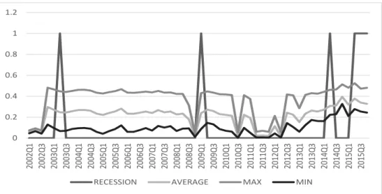
Figure B-3. Recession probabilities with maximum, average and minimum indexes of all ROC models selected (Index1, Index2, Index3, Index4).
4 0 0.2 0.4 0.6 0.8 1 1.2 2 0 0 2 Q 1 2 0 0 2 Q 3 2 0 0 3 Q 1 2 0 0 3 Q 3 2 0 0 4 Q 1 2 0 0 4 Q 3 2 0 0 5 Q 1 2 0 0 5 Q 3 2 0 0 6 Q 1 2 0 0 6 Q 3 2 0 0 7 Q 1 2 0 0 7 Q 3 2 0 0 8 Q 1 2 0 0 8 Q 3 2 0 0 9 Q 1 2 0 0 9 Q 3 2 0 1 0 Q 1 2 0 1 0 Q 3 2 0 1 1 Q 1 2 0 1 1 Q 3 2 0 1 2 Q 1 2 0 1 2 Q 3 2 0 1 3 Q 1 2 0 1 3 Q 3 2 0 1 4 Q 1 2 0 1 4 Q 3 2 0 1 5 Q 1 2 0 1 5 Q 3
RECESSION AVERAGE MAX MIN
Figure B-4. Recession probabilities with average of all ROC models selected (Index1, Index2, Index3, Index4) and leading financial indicator.
5 -0.004 -0.002 0 0.002 0.004 0.006 0.008 0.01 0.012 0 0.2 0.4 0.6 0.8 1 1.2
Figure B-5.Market forecasts of recessions and models selected with out-of-sample ROCs.
6
0.0000 0.1000 0.2000 0.3000 0.4000 0.5000 0.6000 0.7000 0.8000
2003Q2 2009Q1 2014Q2 2015Q2 2015Q3 2015Q4