Ionospheric conductances derived from satellite measurements of auroral UV and X-ray emissions, and ground-based electromagnetic data: a comparison

SRef-ID: 1432-0576/ag/2005-23-343 © European Geosciences Union 2005

Annales

Geophysicae

Ionospheric conductances derived from satellite measurements of

auroral UV and X-ray emissions, and ground-based electromagnetic

data: a comparison

A. Aksnes1, O. Amm2, J. Stadsnes1, N. Østgaard3,1, G. A. Germany4, R. R. Vondrak5, and I. Sillanp¨a¨a2

1_{Department of Physics and Technology, University of Bergen, Bergen, Norway}

2_{Finnish Meteorological Institute, Geophysical Research Division, P.O. Box 503, FIN–00101 Helsinki, Finland} 3_{University of California, Berkeley, CA 94720-7450, USA}

4_{University of Alabama in Huntsville, AL 35899, USA}

5_{NASA/Goddard Space Flight Center, Greenbelt, MD 20771, USA}

Received: 17 January 2004 – Revised: 5 October 2004 – Accepted: 19 October 2004 – Published: 28 February 2005

Abstract. Global instantaneous conductance maps can be derived from remote sensing of UV and X-ray emissions by the UVI and PIXIE cameras on board the Polar satellite. An-other technique called the 1-D method of characteristics pro-vides mesoscale instantaneous conductance profiles from the MIRACLE ground-based network in Northern Scandinavia, using electric field measurements from the STARE coherent scatter radar and ground magnetometer data from the IM-AGE network. The method based on UVI and PIXIE data gives conductance maps with a resolution of ∼800 km in space and∼4.5 min in time, while the 1-D method of charac-teristics establishes conductances every 20 s and with a spa-tial resolution of∼50 km. In this study, we examine three periods with substorm activity in 1998 to investigate whether the two techniques converge when the results from the 1-D method of characteristics are averaged over the spatial and temporal resolution of the UVI/PIXIE data.

In general, we find that the calculated conductance sets do not correlate. However, a fairly good agreement may be reached when the ionosphere is in a state that does not ex-hibit strong local turbulence. By defining a certain tolerance level of turbulence, we show that 14 of the 15 calculated con-ductance pairs during relatively uniform ionospheric condi-tions differ less than±30%. The same is true for only 4 of the 9 data points derived when the ionosphere is in a highly turbulent state. A correlation coefficient between the two conductance sets of 0.27 is derived when all the measure-ments are included. By removing the data points from time periods when too much ionospheric turbulence occurs, the correlation coefficient raises to 0.57. Considering the two very different techniques used in this study to derive the con-ductances, with different assumptions, limitations and scale sizes, our results indicate that simple averaging of mesoscale results allows a continuous transition to large-scale results.

Correspondence to:A. Aksnes (arve.aksnes@ift.uib.no)

Therefore, it is possible to use a combined approach to study ionospheric events with satellite optical and ground-based electrodynamic data of different spatial and temporal reso-lutions. We must be careful, though, when using these two techniques during disturbed conditions. The two methods will only give results that systematically converge when rel-atively uniform conditions exist.

Key words. Ionosphere (Auroral ionosphere; Particle pre-cipitation; Instruments and techniques)

1 Introduction

Knowledge of the ionospheric conductivity is needed to un-derstand the ionospheric electrodynamics and the dynami-cal magnetosphere-ionosphere (MI) coupling. The height-integrated Hall and Pedersen conductivities can be strongly enhanced during auroral substorms, when the particle pre-cipitation increases the electron density in theE-layer. The ionospheric conductivity pattern is complicated, though, as the precipitation may vary strongly in time and space.

The Hall and Pedersen conductivities, σH and σP, can be derived using the classical expressions (Krall and Triv-elpiece, 1973):

σH = Nee B (

2_e ν_en2_⊥+2_e −

2_i

ν_in2 +2_i ) (1)

σP =Nee B (

νini ν_in2 +2_i +

νen⊥2_e

ν_en2_⊥+2_e), (2) where e denotes the elementary charge, νen⊥ represents

Note that Eqs. (1) and (2) are applied to a pseudo-ion aver-age (Brekke, 1997), derived by proper weighting of all ions. The most critical parameter, though, is the electron density Ne. During an auroral substorm,Ne may vary strongly, re-sulting in large spatial and temporal changes in the conduc-tivities.Neis related to the particle precipitation, and height profiles of the ionization can be estimated using measure-ments from particle detectors on rockets (Marklund et al., 1982; Opgenoorth et al., 1983) and satellites (Vondrak and Robinson, 1985). This procedure involves a theoretical mod-elling of the interaction of the precipitating particles with at-mospheric constituents. Another approach is to calculate the conductivities from measurements ofNeby incoherent scat-ter radars on the ground. Numerous studies in the liscat-terature have performed such an investigation, including incoherent scatter radar measurements from Chatanika (Brekke et al., 1974; Banks and Doupnik, 1975; Wedde et al., 1977; de la Beaujardi`ere et al., 1981; Kamide and Vickrey, 1983; Robin-son and Vondrak, 1984), Sondrestrom (RobinRobin-son et al., 1987; Watermann et al., 1993;), and EISCAT (Buchert et al., 1988; Schlegel, 1988; Brekke et al., 1989; Senior, 1991; Olsson et al., 1996; L¨uhr et al., 1998; Davies and Lester, 1999).

An advantage with both in-situ particle measurements on rockets or satellites, andNecalculated from incoherent scat-ter radars, is the high resolution in time and space. The dis-advantage, though, is that only local measurements can be obtained. To provide a global map of conductances, remote sensing of visible, ultraviolet and X-ray emissions produced by the precipitating particles has been shown to be a powerful tool.

Kamide et al. (1986) used images of auroral emissions ob-served with the Dynamic Explorer (DE)-1 satellite to calcu-late ionospheric height-integrated conductivities, or conduc-tances, over the polar region with a 12-min time resolution. A direct empirical relationship between the conductances and the auroral ultraviolet (UV) emission intensity was as-sumed, in order to perform the calculations. Lummerzheim et al. (1991) also used auroral images from the DE-1 satellite to produce global conductance patterns. Their technique to calculate the height-integrated conductivities was somewhat different, as they first derived the characteristic energy and flux of the incoming particles from UV (OI lines at 130.4 and 135.6 nm) and visible (557.7 nm) emissions. Then a method developed by Rees et al. (1988) was used in order to convert the energy spectra to conductance values.

The precipitating electron energy determines the height region of energy deposition, being at lower altitudes with higher energies (Rees, 1963). The intensity of the short-est UV-emission wavelengths escaping the atmosphere de-creases strongly due to absorption of O2, when produced by

energetic electrons depositing their energy too low in the at-mosphere (Lummerzheim et al., 1991; Germany et al., 1990; 1998b). This means that measurements of UV-emissions are unable to accurately characterize the most energetic elec-trons of more than∼10 keV (Robinson and Vondrak, 1994). Østgaard et al. (2001; 2002) combined UV-emissions from the Ultraviolet Imager (UVI) and X-ray data from the Polar

Ionospheric X-ray Imaging Experiment (PIXIE) on board the Polar satellite, to derive global maps of the precipitating elec-tron energy spectra in an energy range of∼0.1–100 keV. By using a computer code based on the TANGLE code (Vondrak and Baron, 1976; Vondrak and Robinson, 1985), Aksnes et al. (2002; 2004) used this data base to derive height profiles of the ionization and the height-integrated conductivities by applying the empirical formulas given in Eqs. (1) and (2). It was found that UV measurements are sufficient to charac-terize the lower electron energies contributing to the Peder-sen conductance, while X-ray measurements are needed to characterize the energetic electrons affecting the Hall con-ductance.

Another approach to derive the ionospheric conductances is to make use of simultaneous ground magnetic and iono-spheric electric field data. The disturbances of the magnetic fieldB measured on the ground depends on the horizontal electric current densityJ flowing in the ionosphere, which is related to the electric fieldEthrough Ohm’s law involving the Hall and Pedersen conductances.

Applying a “trial and error scheme” (e.g. Baumjohann et al., 1981; Opgenoorth et al., 1983) different values of the conductances are combined with models of the ground mag-netic and ionospheric electric field until the calculated and measured magnetic disturbances converge to a sufficient de-gree. The method is applicable even during periods with very poor data coverage, but the method does not give unique so-lutions and no error estimates can be calculated. Another problem with the “trial and error” approach is that the elec-trodynamical parameters must be modelled on a much larger area than the region of interest to reproduce magnetic distur-bances. This often requires that one has to assume a station-ary structure moving with a certain velocity over the field of view of the measurements.

Another technique to investigate the electrodynamics is the method of characteristics (Inhester et al., 1992; Amm, 1995; 1998; Sillanp¨a¨a, 2002). This is a forward modelling method which gives more precise results than the “trial and error” approach (Untiedt and Baumjohann, 1993). Using measurements of the ground magnetic and ionospheric elec-tric field to solve a first-order differential equation, the Hall conductance is derived. By then assuming a ratio between the Hall and Pedersen conductances, the remaining electrody-namical quantities are inferred. There are regions where the solutions using the method of characteristics are not unique. Such regions, though, are known and estimates of the errors can be made. Another advantage compared with the “trial and error” approach is that no data are needed outside the region of interest.

com-parison studies exist in the literature (e.g. Basu and Jasperse, 1987; Vondrak et al., 1988; Senior, 1991; Watermann et al., 1993; Doe et al., 1997; Germany et al., 1997; Dymond et al., 2001; Østgaard et al., 2001). Such studies are complicated when the stochastical processes operate on different scales. Given two methods that measure a parameter with different spatial resolution, it is not a priori clear that an averaging of the results of the method with finer resolution reproduces the ones of the method with coarser resolution. This pos-sible scale-dependency has not been given much attention, though, in earlier papers. For a detailed mathematic formula-tion in terms of properties of statistical processes, the reader is referred to work by Christakos (1992).

In this paper, we derive and compare the ionospheric Hall and Pedersen conductances above Northern Scandinavia us-ing two different techniques. The first method is the proce-dure by Aksnes et al. (2002; 2004), based on remote sensing of UV and X-ray emissions from space, as well as the clas-sical expressions of the conductivities given in Eq. (1) and Eq. (2). This technique will be described more thoroughly in Sect. 2.1. The other procedure is the method of charac-teristics (Inhester et al., 1992; Amm, 1995; 1998, Sillanp¨a¨a, 2002), based on measurements of ground magnetic and iono-spheric electric fields. We will use a version of the procedure named the one-dimensional (1-D) method of characteristics (Inhester et al., 1992; Sillanp¨a¨a, 2002), in which we assume 1-D conditions, i.e. vanishing gradients along a certain direc-tion within the region of investigadirec-tion. A detailed descrip-tion is given in Sect. 2.2. While the former method provides data on a large-scale resolution (∼800 km), integrated over typically 5 min, the 1-D method of characteristics operates with mesoscale resolution (∼50 km) and having values every 20 s. A comparison between the two methods requires that individual conductances from the latter technique must be averaged. The main objective of this paper is to investigate whether simple averaging of the mesoscale results allows a continuous transition to the large-scale results. Such a transi-tion is not obvious regarding the two sets of conductances as results of stochastical processes operating on different scales. Using data from three periods with substorm activity in 1998, we have examined the relationship between the conductances resulting from the two methods to see if the results converge when averaged over the same spatial and temporal scales. Results are presented and discussed in Sect. 3. A summary is given in Sect. 4, while Sect. 5 provides the conclusions of this study.

2 Deriving ionospheric conductances

2.1 Technique 1: Remote sensing from space of UV and X-ray emissions

Through remote sensing of UV and X-ray emissions from space, the precipitating electron energy spectra can be de-rived. By then estimating height profiles of the resulting ionization, ionospheric Hall and Pedersen conductances are

obtained. A detailed description of this method is given by Aksnes et al. (2002; 2004), as well as a discussion of its limitation (Aksnes et al., 2004). Here we just give a brief description of the method.

The UVI camera (Torr et al., 1995) on the Polar satellite measures UV-emissions within the Lyman-Birge-Hopfield (LBH) band (140–180 nm). These UV-emissions are sepa-rated into LBHS (140–160 nm) and LBHL (160–180 nm). As the shortest wavelengths (LBHS) are subject to considerably greater absorption in the atmosphere than the longer wave-lengths (LBHL), we can derive the average electron energy from the ratio between the intensities of the two LBH-bands. We can further calculate the electron energy flux from the in-tensity of the LBHL emissions. To accumulate the two LBH images needed to perform an electron energy determination from UVI, it takes on the order of two minutes, depending on the operating sequence. UVI has a nominal spatial reso-lution of∼40 km from apogee (Torr et al., 1995). The spa-tial resolution is degraded in one direction to∼360 km due to wobbling of the Polar satellite. More details about the energy determination from UVI are given by Germany et al. (1997; 1998a,b).

The PIXIE camera (Imhof et al., 1995) measures bremsstrahlung in the energy range of∼2–22 keV, produced when precipitating electrons interact with the nuclei of at-mospheric particles. The X-ray photons detected by PIXIE go through a 4.4-mm pinhole, leaving us with a resolution in the X-ray source region of∼600–900 km (depending on Po-lar altitude). As described by Østgaard et al. (2000; 2001), the X-ray measurements combined with a look-up table pro-duced by a coupled electron-photon transport code (Lorence, 1992) can be used to derive a four-parameter representa-tion of the precipitating electrons from∼3 keV to∼100 keV. These electron spectra are typically 4.5-min averages every 10 min.

The energy characteristics derived from UVI and PIXIE measurements can be combined to give the electron energy distribution from∼0.1 to∼100 keV (Østgaard et al., 2001), with the temporal and spatial resolution of the PIXIE instru-ment (4.5 min and 600–900 km). An upper limit of modelling errors when deriving mean energies from UVI measurements is estimated to be 23% (Germany et al., 2001). Comparing the energy spectra derived from UVI and PIXIE data with in-situ measurements from the Defense Meteorological Satellite Program (DMSP) satellites, Østgaard et al. (2001) found an average ratio of 1.03±0.6 between calculated and measured energy flux from 0.09 keV to 30 keV. One possible explana-tion of the large standard deviaexplana-tion may be the different spa-tial resolutions.

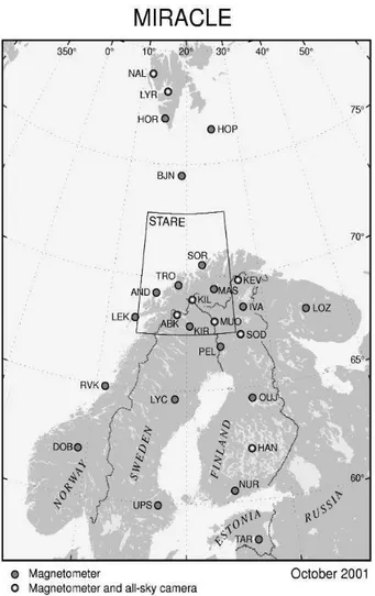
Fig. 1.Map of the MIRACLE network.

collision frequencies are estimated from Itikawa (1971) and Gagnepain et al. (1977), while the ion-neutral collision fre-quencies are derived using work by Mason (1970), Pesnell et al. (1993), and Viehland and Mason (1995).

2.2 Technique 2: 1-D method of characteristics

The ionospheric Hall and Pedersen conductances, 6H and 6P, can be derived using measurements of the ionospheric electric fieldEand the ground magnetic fieldB. The method is called the method of characteristics, as it solves a differen-tial equation along its characteristics. In this study, we will apply this technique using electric field measurements from the Scandinavian Twin Auroral Radar Experiment (STARE) and ground magnetometer data from the International Moni-tor for Auroral Geomagnetic Effects (IMAGE) network.

A map showing the Magnetometers - Ionospheric Radars - Allsky Cameras Large Experiment (MIRACLE) network is presented in Fig. 1. The IMAGE magnetometer sites are indicated as dots, while the STARE field of view (FOV) is marked by the black rectangle. The method of character-istics is described in detail by Inhester et al. (1992), Amm (1995; 1998), and Sillanp¨a¨a (2002). Here, we will only give

a general overview, including the most important equations. Note that we will use the 1-D version of the procedure, as-suming that gradients along a certain direction are vanishing within the region of investigation. We will first introduce the equations related to the two-dimensional (2-D) method of characteristics, and then proceed to the 1-D version.

When using the method of characteristics, the ionosphere is considered an infinitely thin conducting layer 100 km above the Earth’s surface, in which the Hall and Pedersen currents are flowing. The first step is to extract the external part of the ground magnetic field disturbance. A field contin-uation to the ionosphere is then performed (Mersmann et al., 1979; Untiedt and Baumjohann, 1993), and we derive the ionospheric equivalent currentJ_eq,ion. According to Fig. 1

the ground magnetometer data cover only about half the area of STARE. Pulkkinen et al. (2003) have shown, though, that the equivalent currents can be reliably reconstructed in the whole STARE FOV, including those areas which are not in an immediate vicinity of the ground magnetometers.

The true ionospheric current J can be separated into a curl-free component Jcf and a divergence-free component Jdf (Duschek and Hochrainer, 1961). While Jcf is as-sociated with the field-aligned current jz above the iono-sphere, Jdf is related to the horizontal component of the external magnetic field perturbation(Be)h immediately be-low the ionosphere (Untiedt and Baumjohann, 1993). Note that the subscripth indicates the horizontal component of Be. By assuming that the Earth’s geomagnetic field lines are directed vertically downward into thezˆ direction,Jdf will completely determine (Be)h (Bostrøm, 1964; Vasuliunas, 1970; Fukushima, 1976). If the angleχ between the iono-spheric plane and the geomagnetic field lines deviates from 90◦, then there is also some dependence of (Be)h onJcf (Fukushima, 1976). At auroral latitudes, though, it is appro-priate to disregard the tilting between the Earth’s magnetic field with respect to the vertical. The conductance calcula-tions using a typical value ofχ=77◦for the measuring sites in Northern Scandinavia to be compared withχ=90◦have been examined by Amm (1995) during four different situations: a two-dimensional eastward electrojet, a Harang discontinuity, an omega band and a westward travelling surge. The investi-gation by Amm (1995) revealed, with a few exceptions, only minor differences of a few % for most of the examined areas. Another basic electrodynamic equation needed when us-ing the method of characteristics is Ohm’s law. Here we disregard possible effects of the neutral wind (Untiedt and Baumjohann, 1993). We further assume a ratioα between the Hall and Pedersen conductances to be given:

α= 6H 6P

. (3)

con-ductance calculations from UVI and PIXIE (see Sect. 2.1) to determineα.

By combining all the relations established, we can provide a formula giving the Hall conductance6Halong a character-isticr(ℓ), which is a line in the xy-plane:

6H(r(ℓ))=6H(r0)exp[−I (0, ℓ)]

+ Z ℓ

0

D(r(ℓ))

|V(r(ℓ))|exp[−I (ℓ ′

, ℓ)]dℓ′ (4)

with I (ℓ′, ℓ)=

Z ℓ

ℓ′

C(r(ℓ′′))

|V(r(ℓ′′))| (5)

V =E−zˆ×E

α (6)

C= ∇h·V (7)

D= 2 µ0

∇h·(Be)h. (8)

Equation (4) represents the two-dimensional method of char-acteristics, asr(ℓ)lies on the xy-plane. The problem can be much simplified, though, if we assume a one-dimensional sit-uation for which the gradient of all quantities vanishes in one horizontal direction (Inhester et al., 1992; Sillanp¨a¨a, 2002). By taking _δyδ=0 and _δxδℓ=|_VV|

x, we can replace Eqs. (5), (7)

and (8) with: I (ℓ′, ℓ)=ln(Vx(x)

Vx(x′)

) (9)

C= δVx

δx (10)

D= 2 µ0

δBe,x

δx . (11)

Insertion of Eqs. (9), (10) and (11) into Eq. (4) yields the 1-D method of characteristic solution for the Hall conductance :

6H(x)=

2

µ0Be,x+K Vx(x)

(12) The constant K in Eq. (12) represents the effect of distant currents. If for somex0, Vx(x0)=0 holds,Kis uniquely

de-fined. In other cases we use the criterion that at the edges of the electrojet region the conductances drop to a given back-ground value (see Inhester et al., 1993; Sillanp¨a¨a, 2002) to inferK.

In this study, we have used the 1-D method of characteris-tic to derive the ionospheric Hall and Pedersen conductances in the Northern Scandinavian region, having a spatial reso-lution of ∼50 km and a temporal resolution of ∼20 s. As the procedure requires that the electrodynamical parameters only change in one direction within the STARE FOV, investi-gations have been performed to check that the different time steps and regions involved satisfy the 1-D condition. This

means that all quantities should have a vanishing derivative along a certain direction. In our case we assume that this direction is zonal (east-west), while we allow for variations in the meridional direction. The criterion for using the 1-D method is that the changing length of a parameter should be larger than the length of the relevant analysis area in the east-west direction. If the parameter isX, then the changing length is defined asL=|X/(dX_dL)|. The electric field strength must be more than∼17 mV/m for STARE to provide reliable results (Sillanp¨a¨a, 2002). For each time step along each lati-tude for which sufficient STARE data are available, we check whether the electric field is one-dimensional. Regions where this is not the case are excluded from the conductance cal-culation. Another possibility is that the conductances them-selves do not satisfy a 1-D condition. This situation will in most cases, but not all, cause a considerable non-1-D ground magnetic field. Such cases are more difficult to reveal, due to the limited east-west coverage of magnetometer stations within the STARE region (see Fig. 1). A more thorough dis-cussion about this problem is provided in Sect. 3 when in-terpreting the conductance profiles established using the two different techniques.

As shown in this section, the Hall conductance is the pri-mary output from the 1-D method of characteristics, from which other quantities like, for example, field-aligned cur-rents (FACs) can be calculated. In a recent study by Amm et al. (2003), the FACs calculated using the 1-D method of char-acteristics are compared with FAC derived from in-situ mea-surements by the Cluster satellites. By showing a convinc-ing agreement between the two sets of FAC data, Amm et al. (2003) indirectly demonstrate that the Hall conductances derived using the 1-D method of characteristics give reliable results.

2.3 Assumptions and limitations of the two techniques As explained in Sect. 1, the main objective of this paper is to investigate whether simple averaging of mesoscale results (1-D method of characteristics) allows for a continuous tran-sition to large-scale results (the UVI/PIXIE analysis). While the latter technique operates with a resolution of ∼800 km in space and∼4.5 min in time, the ground-based method es-tablishes conductances every 20 s and with a spatial resolu-tion of∼50 km. This comparison is further complicated by several different assumptions and limitations of the two tech-niques.

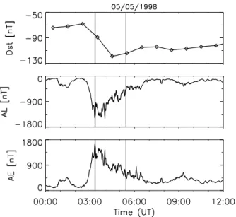
Fig. 2.The AE, AL andDst-indices between 00:00 and 12:00 UT on 5 May 1998. The two vertical solid lines indicate our time inter-val with data between 03:20 and 05:25 UT.

problem occurs when STARE data are unable to provide a reliable electric field value.

As pointed out in Sect. 2.1, the UVI data are responsible for the lower part of the precipitating electron energy spectra up to∼15–20 keV. The estimation of the electron energies using UVI measurements within time periods of∼4.5 min may be affected in two ways. First of all, the LBHL and LBHS images are not coincident as they are measured dur-ing different time intervals of 37 s. In cases where the au-roral morphology is significantly changing between the two observations, this leads to an analysis problem, though the uncertainty is difficult to estimate. A second problem is that the UVI measurements are not continuous within the investi-gated time intervals of∼4.5 min. For example, it takes 1 min and 51 s to perform a full energy analysis from UV-emissions for the operating modes used in this study. Then there is a gap of 1 min and 13 s before the procedure is repeated. If sudden changes in the particle precipitation takes place dur-ing such gaps, this will complicate the comparison with the 1-D method of characteristics.

The resolution of the PIXIE instrument is on the order of∼600–900 km (see Sect. 2.1), depending on the altitude of the Polar satellite. In comparison, the STARE FOV is nominally approximately 470 km×540 km, as it covers a ge-ographic region of 67.1–72.0 in latitude and 14.0–26.0 in longitude. For two of the three events studied in this paper, the most equatorward region has been left out of the analy-sis, due to a very limited number of ion velocity vectors pro-duced by the two radar beams. This reduces the latitudinal width from 540 km to 380 km. The inconsistency between the PIXIE’s resolution and the STARE’s FOV leads to an-other source of uncertainty which is discussed in more detail in Sect. 3.

2.4 Selection of data

Three periods with substorm activity in 1998 have been se-lected for this study. The two events of 5 May and 26 June 1998, include data from parts of the substorm expansion phase and most of the recovery phase. For the 12 August 1998 event, we have measurements from the start of sub-storm onset until the beginning of the recovery phase.

A number of only three events for a comparison study may seem low, but is due to a variety of reasons. First of all, to use the 1-D method of characteristics, the STARE radars must re-ceive enough backscatter to estimate the electric field. Most of the time STARE sees no echoes at all. Either there are too few electrons in the critical altitude range, or the electric field is too weak to form irregularities. While the former im-ply that substorm periods should be most suited for studies using STARE, the latter suggest that problems may some-times occur during the substorm expansion phase, when the electron density and therefore also the conductances can be extremely high in some small volume. If the magnetosphere acts as a current generator, this can lead to a suppression of the electric field to very small values below the threshold of the radars. In general, though, STARE is well suited to in-vestigate the electrodynamics during substorms, and so are also instruments performing remote sensing from space. A comparison between the two techniques, however, requires that the Polar satellite for the time period of interest is lo-cated above the Northern Hemisphere, with the UVI and PIXIE instruments viewing the Scandinavian region. Sub-storm conditions are best suited, as we need to detect suf-ficient X-ray photons by PIXIE to derive a proper electron spectrum. The UVI camera, which can operate in different modes to investigate certain aspects of the auroral activity, must further operate in a special mode if a full energy anal-ysis is to be performed. The most critical requirement lim-iting the number of possible events, though, is the fact that we have only considered the date period between May and September, 1998. While the Finnish STARE radar station Hankasalmi suffered from hardware problems in 1997 and the beginning of 1998, the PIXIE chamber detecting X-ray photons between∼8–22 keV was no longer functioning after 30 September 1998. PIXIE continued to detect X-ray pho-tons between∼2–8 keV until November 2002, but the lack of information about the most energetic X-rays strongly in-creased the uncertainty in estimating the high energy tail of the precipitating electrons up to 100 keV affecting the Hall conductance (Aksnes et al., 2002; 2004).

3 Results and discussion

3.1 5 May 1998

respectively, theDst-diagram show that we are in the main phase of a geomagnetic storm. A minimum in Dst of −119 nT between 04:00 and 05:00 UT means this event is classified as an intense storm (Gonzalez et al., 1994). We have estimated the conductances between 03:20 and 05:25 UT, as indicated by the two vertical solid lines. This time interval includes parts of the expansion phase and then the recovery phase.

The results of the conductance calculations using the two techniques including remote sensing of UV and X-ray emis-sions (see Sect. 2.1) and the 1-D method of characteristics (see Sect. 2.2) are presented in Fig. 3. The solid lines in Figs. 3a and b indicate the Hall and Pedersen conductances derived from the UVI/PIXIE analysis, while the dashed lines represent the conductances using the 1-D method of charac-teristics. The conductance values are 10 min apart, with an integration time of about 4.5 min. For this event, the STARE radar measurements are taken from a geographic region of 67.1–72.0 in latitude and 14.0–26.0 in longitude, meaning that the STARE FOV is approximately 470 km×540 km.

In the beginning of the investigated time interval, we ob-serve differences between the two conductance profiles in both magnitude and trend. The values derived using the 1-D method of characteristics show most variability, with a maxi-mum Hall conductance of 33 S at 04:00–04:05 UT and a min-imum 20 min later of only 11 S. For this time step, the con-ductances using ground-based measurements are more than 60% less than the values derived from remote sensing of UV and X-ray emissions. This is clearly indicated by the plot in Fig. 3c, showing the differences in % when calculating the conductances using the 1-D method of characteristics in-stead of using UVI/PIXIE data. As explained in Sect. 2.2, the Pedersen conductance calculated using the 1-D method of characteristics depends on the ratioα between the Hall and the Pedersen conductances derived from the UVI/PIXIE analysis. Consequently, the percentages given in Fig. 3c cor-respond to both the differences between the two Hall conduc-tance sets in Fig. 3a, as well as the differences between the two Pedersen conductance sets in Fig. 3b.

In the next time frame of 04:30–04:35 UT, a shear region intrudes into the STARE FOV. This causes a considerable dropout of STARE data, and therefore this time step is left out in the analysis. For the rest of the time period from 04:40 until 05:25 UT, the two conductance profiles match fairly well, except for the time step of 04:50–04:55 UT.

As described in Sect. 2.3, the different assumptions and limitations of the two techniques imply that a meaningful comparison relies strongly on the level of turbulence of the ionosphere. We have therefore developed a method to sep-arate the data points into relatively uniform conditions and non-uniform conditions. Relatively uniform conditions are considered to be present if the following three selection crite-ria are fulfilled: 1) More than 70% of the individual magnetic scale lengths must be larger than 429 km. 2) The largest UVI-inhomogeneity within the STARE FOV must be less than 100%. 3) The difference between the average UVI inten-sity within the STARE FOV vs. a larger region of∼800 km

03:00 03:30 04:00 04:30 05:00 05:30

Time [UT]

03:00 03:30 04:00 04:30 05:00 05:30

Time [UT]

Difference [%] in

UVI-emission values

STARE FOV vs PIXIE res.

-40 -20 0 20

40 0

50 100 150 200

Difference [%] MIN vs MAX

UVI-emission values

Mag Scale Length [km]

100 1000

10000 -100

-50 0 50 100

Difference

[%]

Pedersen

Conductance [S]

0 5 10 15 20

05/05/1998 05/05/1998

0 10 20 30 40

Hall

Conductance [S]

(a)

(b)

(c)

(d)

(e)

(f)

Fig. 3.(a)The Hall and(b)Pedersen conductances [S] derived in the Scandinavian region using UVI and PIXIE measurements (solid line) and the 1-D method of characteristics (dashed line) on 5 May

1998. (c)The difference in % between the two conductance sets.

The horizontal dashed line is drawn to give the 0-percent level, while the length of the lines indicates the integration time period.

(d)Magnetic field scale lengths (km) between the two MIRACLE

magnetometer stations of AND and KEV.(e)The average

percent-age calculated using the lowest and largest UVI-LBHL emission

values at five strips of constant latitude within the STARE FOV.(f)

The difference in % for the average UVI-LBHL intensity within the STARE FOV compared with the average UVI-LBHL intensity when including a larger area surrounding the STARE FOV match-ing the PIXIE resolution.

(the PIXIE resolution) must be less than 20%. A detailed de-scription of these three selection criteria will be given in the following when discussing Fig. 3.

14 18 22 26

69 71

73

< >

89 269 448 627 807 986 1166 1345 1525 1704 1883 2063 [R]

12 16 20 24 28

68 70

72 74

980505 042330-042407 UT

✁

14 18 22 26

69 71

73

< >

105 315 525 735 946 1156 1366 1577 1787 1997 2207 2418 [R]

12 16 20 24 28

68 70

72 74

980505 042634-042711 UT

Fig. 4. The UVI-LBHL images for the two time steps of (a)

04:23:30–04:24:07 UT and(b)04:26:34–04:27:11 UT on 5 May

1998. The inner black box drawn on top of the images corresponds to the STARE FOV, while the outer box matches the PIXIE

resolu-tion of∼800 km.

and Kevo (KEV), which are located at almost the same geo-graphic latitude (∼69.3 and∼69.8◦, respectively). When the calculated magnetic scale lengths are smaller than a heuristi-cal limit of∼429 km (the extent of the east-west chain AND-KEV), this means we may not have a 1-D condition. For such a situation, we should be careful when interpreting the conductances using the 1-D method of characteristics. All data within the STARE FOV are still included in the con-ductance calculation, as the investigation performed only in-volves the conditions between AND and KEV. Other regions within the STARE FOV are not investigated, as the limited

east-west coverage of magnetometer stations prevents an ef-ficient check similar to the procedure regarding the electric field.

In Fig. 3d, we present magnetic scale lengths estimated between AND and KEV for the different time periods. The scale lengths are calculated every 20 s, and we plot the in-dividual values in km as solid lines for the different time steps. We observe that the values are usually larger than the heuristical limit of∼429 km shown by a dashed horizontal line, indicating that our assumption of a 1-D condition holds. During some time intervals, though, many of the individual scale lengths drop below 429 km, suggesting more disturbed conditions. Our first selection criterion requests that more than 70% of the individual magnetic scale lengths (in the ∼5 min time frames) must be larger than the heuristical limit of 429 km. This is fulfilled for the first four time steps, as well as the last four. During the period∼04:00–04:45 UT, however, the investigation of magnetic scale lengths indi-cates too much ionospheric turbulence.

The second selection criterion also deals with the neces-sary 1-D condition for the 1-D method of characteristics. We have used UVI-LBHL measurements to monitor changes in precipitated energy flux. First, we have divided the STARE FOV into a 5×4 grid, with each subregion being 1◦in latitude and 3◦in longitude. Then we have calculated the differences in % between the lowest and the largest UVI intensities along each of the five strips of constant latitude. Based on these five individual values derived for the latitude sectors of 67–68◦, 68–69◦, 69–70◦, 70–71◦, and 71–72◦respectively, an aver-age percentaver-age value has been established for each UVI data set, having a temporal resolution of 37 s. For simplicity, we will refer to such values as ”UVI-inhomogeneities” through-out the text.

The results are presented in Fig. 3e. In the beginning of the time interval, the UVI-inhomogeneities are usually less than 50%. The first minor intensification is found at 03:34 UT, when the value reaches 62%. Throughout the next hour, we observe an increasing trend of the UVI-inhomogeneities, co-inciding with a reduction of the magnetic scale lengths pre-sented in Fig. 3d. Between∼04:00 and 04:30 UT, the UVI-inhomogeneities sometimes exceed 100% while the scale lengths drop below∼429 km.

In Figs. 4a and b, we have plotted the UVI images for the two time steps of 04:23:30–04:24:07 UT and 04:26:34– 04:27:11 UT. The inner black box drawn on top of each im-age indicates the STARE FOV, while the outer box corre-sponds to a region of ∼800 km, matching the PIXIE reso-lution. Note that the colors in the two plots correspond to different intensities, as the dark red color is set equal to the maximum value in each plot.

Such variability in the east-west direction complicates the calculation of conductances when using the 1-D method of characteristics. Our second selection criterion to iden-tify relatively uniform conditions requires that the UVI-inhomogeneities must be below 100%. This means that the time steps of∼03:50–03:55 and ∼04:50–04:55 UT should also be assigned non-uniform conditions, in addition to the time period of∼04:00–04:45 already determined from the previous investigation of magnetic scale lengths (Fig. 3d).

The third selection criterion deals with the difference be-tween the STARE FOV and the much coarser PIXIE resolu-tion. From the image given in Fig. 4a, we note a significant UVI intensity surrounding the STARE region. For this event on 5 May 1998, the PIXIE resolution of ∼800 km corre-sponds to an area about 2.5 times larger than the STARE FOV of 470 km×540 km. The inconsistency between the PIXIE resolution and the STARE’s FOV implies that the conditions in the particle precipitation outside the STARE region may influence the PIXIE measurements and therefore affect the conductance calculation. This possible source of error has been studied by investigating the UVI-LBHL emissions in a region larger than the actual analyzing area. The much better spatial and temporal resolution given by the UVI camera pro-vides us with a tool to investigate the reliability of the PIXIE data. First, we have calculated the average UVI-LBHL in-tensity within the STARE FOV, a region corresponding to the inner black box in Fig. 4. Then we have repeated the calculation and taken into account a larger area surrounding the STARE FOV matching the PIXIE resolution. This larger region corresponds to the outer black box in Fig. 4.

In Fig. 3f, we present the differences in % between the UVI intensities derived using the two approaches. Nega-tive values mean that the average UVI intensity is largest within the STARE FOV. Since regions with less precipitation surrounding the STARE FOV matching the PIXIE resolu-tion also influence the X-ray data, we may underestimate the conductances using UVI/PIXIE data during such situations. Likewise, positive values in Fig. 3f indicate stronger particle precipitation outside the region of investigation and a possi-ble overestimation of the conductances when using the satel-lite data. By comparing the results in Figs. 3c and f, we note some resemblance between the values. Around∼04:00 UT, we observe the lowest value in Fig. 3f of less than−20%. At this time the conductances using the 1-D method of char-acteristics are almost 30% larger than the conductances us-ing UVI/PIXIE data. Then the situation is reversed around 04:23 UT. The 1-D values are more than 60% less than the satellite calculations and Fig. 3f reveals a positive value of about 30%. Our third selection criterion states that the dif-ference between the average UVI intensity for a region corre-sponding to the STARE FOV vs. a larger region of∼800 km (the PIXIE resolution) must be below 20%. This means that the two time steps of 04:00–04:05 and 04:20–04:25 UT must be classified as periods when the ionosphere is in a highly turbulent state. Both time steps have already been assigned non-uniform conditions, though, based on the previous anal-ysis of magnetic scale lengths and UVI-inhomogeneities.

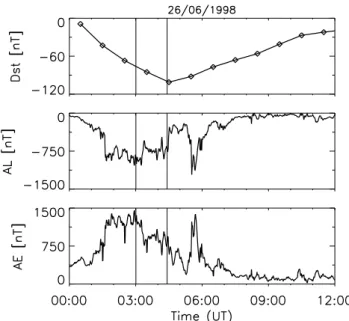
Fig. 5.The AE, AL andDst-indices between 00:00 and 12:00 UT on 26 June 1998. The two vertical solid lines indicate our time interval with data between 03:00 and 04:15 UT.

By performing several investigations and requiring that certain selection criteria associated with each of them are fulfilled, we are able to identify time periods when a bet-ter match between the two conductance sets should be ex-pected. Using different methods is helpful, as each proce-dure has its advantages as well as disadvantages. For exam-ple, the magnetic scale lengths are estimated continuously, while the UVI-inhomogeneities are calculated every 2 min with an integration time of 37 s. While this suggests that it should be sufficient to only deal with the former, the mag-netic scale lengths have a limited spatial coverage compared with UVI. Consequently, the latter procedure may reveal dis-turbed conditions not captured by the analysis of magnetic scale lengths.

To distinguish between the data points during relatively uniform conditions and non-uniform conditions, the latter has been marked with a dark grey shading in Fig. 3. For 5 of the 6 time steps when all three selection criteria are fulfilled, the differences between the two conductance sets are less than±30%. On the contrary, only 3 of the 6 time steps dur-ing non-uniform conditions between∼03:45 and 05:00 UT reveal conductances within±30%.

3.2 26 June 1998

03:00 03:15 03:30 03:45 04:00 04:15 Time [UT]

03:00 03:15 03:30 03:45 04:00 04:15

Time [UT]

Difference [%] in

UVI-emission values

STARE FOV vs PIXIE res.

-40 -20 0 20

40 0

50 100 150 200

Difference [%] MIN vs MAX

UVI-emission values

Mag Scale Length [km]

100 1000

10000 -100

-50 0 50 100

Difference

[%]

Pedersen

Conductance [S]

0 5 10 15 20

26/06/1998 26/06/1998

0 10 20 30 40

Hall

Conductance [S]

(a)

(b)

(c)

(d)

(e)

(f)

Fig. 6.(a)The Hall and(b)Pedersen conductances [S] derived in the Scandinavian region using UVI and PIXIE measurements (solid line) and the 1-D method of characteristics (dashed line) on 26 June

1998. (c)The difference in % between the two conductance sets.

The horizontal dashed line is drawn to give the 0-percent level, while the length of the lines indicates the integration time period.

(d)Magnetic field scale lengths (km) between the two MIRACLE

magnetometer stations of AND and KEV.(e)The average

percent-age calculated using the lowest and largest UVI-LBHL emission values at four strips of constant latitude within the STARE FOV.

(f)The difference in % for the average UVI-LBHL intensity within

the STARE FOV compared with the average UVI-LBHL intensity when including a larger area surrounding the STARE FOV match-ing the PIXIE resolution.

following recovery phase. As the Dst-index value reaches a minimum of−101 nT between 04:00 and 05:00 UT, we further note that we are in the main phase of an intense geo-magnetic storm.

In Figs. 6a and b we present the calculated Hall and Peder-sen conductances similar to Figs. 3a and b. The STARE radar measurements for this event have a lower latitude limit of 68.6◦, resulting in a STARE FOV of about 470 km×380 km. Highly disturbed ionospheric conditions occur for the three time periods between∼03:10 and 03:40 UT, as indicated by the dark grey area in Fig. 6. During the remaining 5 time periods, the ionosphere is in an appropriate state considering our three selection criteria presented in Sect. 3.1.

As seen in Fig. 6c, two of the time intervals, 03:20–03:25 and 03:30–03:35 UT, show differences between the derived conductances of −55 and 80%, respectively. This may be explained by a lack of 1-D conditions. According to Fig. 6d,

more than 50% of the individual magnetic scale length val-ues are below the heuristical limit of∼429 km between 03:20 and 03:25 UT. We further observe in Fig. 6e that the inves-tigation of UVI intensities along strips of constant latitude within the STARE FOV reveals the largest differences dur-ing the time interval of 03:25 and 03:35 UT, varydur-ing between ∼100 and∼160%. Consequently, these two time periods of 03:20–03:25 and 03:30–03:35 UT are assigned non-uniform conditions.

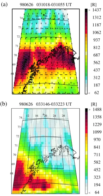
The UVI images for the two time steps of 03:10:18– 03:10:55 UT and 03:31:46–03:32:23 UT are plotted in Figs. 7a and b. Fairly stable conditions in the east-west di-rection are found in the first image, suggesting that the 1-D condition holds for the start of the time step of∼03:10– 03:15 UT. This is supported by individual magnetic scale lengths of∼1400 km. After a maximum scale length of more than 2000 km around 03:11 UT, the values decrease strongly and reach a minimum of 218 km (Fig. 3d). Only∼50% of the individual scale lengths are larger than 429 km within the time frame of∼03:10–03:15 UT, meaning that selection cri-terion No. 1 is not fulfilled.

Figure 7b reveals large variations along the strips of constant latitude, corresponding well with the UVI-inhomogeneities in Fig. 6e, exceeding 100% at these times. Consequently, the time step of ∼03:30–03:35 UT is at-tributed to non-uniform ionospheric conditions. This is also reflected in the investigation of the differences between the average UVI intensity for a region of 470 km×380 km (the STARE FOV) and∼800 km (the PIXIE resolution), respec-tively. As shown in Fig. 6f, the largest differences of more than 20% occur between∼03:20 and 03:40 UT.

Our analysis of the local ionospheric turbulence for this event on 26 June 1998, shows that non-uniform conditions appear during the three time steps between ∼03:10 and ∼03:40 UT. Only 1 of the 3 calculated conductance sets dur-ing this time period differs less than ±30%. On the con-trary, all 5 time steps when we have relatively uniform iono-spheric conditions provide conductances with differences within±30%.

3.3 12 August 1998

Figure 8 presents the geomagnetic indices AE, AL andDst, between 20:00 and 08:00 UT on 12–13 August 1998. In the beginning of the time period, when we have measurements between 23:30 and 23:55 UT on 12 August, we observe a sig-nificant increase in the AE- and AL-indices. The largest val-ues are found around 23:40 UT, when AE reaches∼650 and AL exceeds−400 nT. Then the magnetic activity decreases at the end of the time period, suggesting that our time in-terval of 23:30–23:55 UT includes the substorm expansion phase and the start of the recovery phase. We further note that no geomagnetic storm is present, as theDst-values are small.

14 18 22 26

69 71

73

< >

62 187 312 437 562 687 812 937 1062 1187 1312 1437

[R]

(a)

12 16 20 24 28

68 70

72 74

980626 031018-031055 UT

✁

14 18 22 26

69 71

73

< >

64 194 323 452 582 711 841 970 1099 1229 1358 1488

[R]

(b)

12 16 20 24 28

68 70

72 74

980626 033146-033223 UT

Fig. 7. The UVI-LBHL images for the two time steps of (a)

03:10:18–03:10:55 UT and(b)03:31:46–03:32:23 UT on 26 June

1998. The inner black box drawn on top of the images corresponds to the STARE FOV, while the outer box matches the PIXIE

resolu-tion of∼800 km.

similar to the event on 26 June 1998. The two conductance profiles are much alike. Both the magnetic scale lengths (Fig. 9d) and the UVI-inhomogeneities (Fig. 9e) indicate that the 1-D condition holds.

In Figs. 10a and b, we have plotted the UVI images for the two time steps of 23:41:58–23:42:35 UT and 23:45:02– 23:45:39 UT. Both images reveal more or less uniform con-ditions, with the latter changing only 10% in UVI intensity in the east-west direction within the STARE FOV. The two im-ages also suggest uniform conditions throughout the entire region of∼800 km, as the situation is much the same within

Fig. 8.The AE, AL andDst-indices between 20:00 and 08:00 UT on 12–13 August 1998. The two vertical solid lines indicate our time interval with data between 23:30 and 23:55 UT.

the outer black box corresponding to the PIXIE resolution. We therefore see in Fig. 9f that the differences in % between the average UVI intensity for a region of 470 km×380 km (the STARE FOV) and∼800 km (the PIXIE resolution) are practically 0. The results show that all four time steps occur during relatively uniform ionospheric conditions, and that all the conductance sets provide differences of less than±30%.

4 Summary

23:30 23:35 23:40 23:45 23:50 23:55 Time [UT]

23:30 23:35 23:40 23:45 23:50 23:55

Time [UT]

Difference [%] in

UVI-emission values

STARE FOV vs PIXIE res.

-40 -20 0 20

40 0

50 100 150 200

Difference [%] MIN vs MAX

UVI-emission values

Mag Scale Length [km]

100 1000

10000 -100

-50 0 50 100

Difference

[%]

Pedersen

Conductance [S]

0 5 10 15 20

12/08/1998 12/08/1998

0 10 20 30 40

Hall

Conductance [S]

(a)

(b)

(c)

(d)

(e)

(f)

Fig. 9.(a)The Hall and(b)Pedersen conductances [S] derived in the Scandinavian region using UVI and PIXIE measurements (solid line) and the 1-D method of characteristics (dashed line) on 12

Au-gust 1998. (c)The difference in % between the two conductance

sets. The horizontal dashed line is drawn to give the 0-percent level, while the length of the lines indicates the integration time period.

(d)Magnetic field scale lengths (km) between the two MIRACLE

magnetometer stations of AND and KEV.(e)The average

percent-age calculated using the lowest and largest UVI-LBHL emission values at four strips of constant latitude within the STARE FOV.

(f)The difference in % for the average UVI-LBHL intensity within

the STARE FOV compared with the average UVI-LBHL intensity when including a larger area surrounding the STARE FOV match-ing the PIXIE resolution.

UVI/PIXIE∼4.5-min intervals and in space over the STARE FOV.

The results presented in Sect. 3 reveal that the two tech-niques used to derive the conductances sometimes provide similar values. Other times, however, the conductances can differ strongly. For the events on 5 May and 26 June 1998, the best correspondence between the two conductance sets is found at the end of the investigated time periods, when we are in the late recovery phase of a substorm. Then the geo-magnetic conditions are less disturbed.

An even better agreement is found for the conductances derived on 12 August 1998. As shown in Fig. 8, we start out in the substorm expansion phase, followed by the beginning of the recovery phase. The AE and AL indices, though, are moderate compared to the other two events. We further note that this substorm takes place during non-storm conditions, while the events on 5 May and 26 June 1998, occurred during the main phase of an intense geomagnetic storm.

14 18 22 26

69 71

73

< >

43 130 216 303 390 476 563 650 736 823 910 996 [R]

(a)

12 16 20 24 28

68 70

72 74

980812 234158-234235 UT

✁

14 18 22 26

69 71

73

< >

35 107 179 250 322 393 465 537 608 680 752 823

[R]

(b)

12 16 20 24 28

68 70

72 74

980812 234502-234539 UT

Fig. 10. The UVI-LBHL images for the two time steps of (a)

2341:58-2342:35 UT and(b)23:45:02–23:45:39 UT on 12 August

1998. The inner black box drawn on top of the images corresponds to the STARE FOV, while the outer box matches the PIXIE

resolu-tion of∼800 km.

This has led to the separation of the different conductance values presented in Figs. 3, 6 and 9, according to their cor-responding ionospheric conditions. Relatively uniform con-ditions have been attributed to situations when the follow-ing selection criteria are fulfilled: 1) More than 70% of the individual magnetic scale lengths (Figs. 3d, 6d, 9d) must be larger than 429 km. 2) The largest UVI-inhomogeneity within the STARE FOV (Figs. 3e, 6e, 9e) must be less than 100%. 3) The difference between the average UVI intensity (Figs. 3f, 6f, 9f) within the STARE FOV vs. a larger region of∼800 km (the PIXIE resolution) must be less than 20%.

For the event on 5 May we find that 6 time periods may be attributed to relatively uniform conditions. Five of these cases provide conductances with differences of less than ±30%. The same holds true for the 5 time steps with lo-cal turbulence below our tolerance limit during the event on 26 June, as well as all 4 values taken from 12 August. On the contrary, only 4 of the conductance pairs from the remaining 9 periods with non-uniform conditions reveal differences of less than±30%.

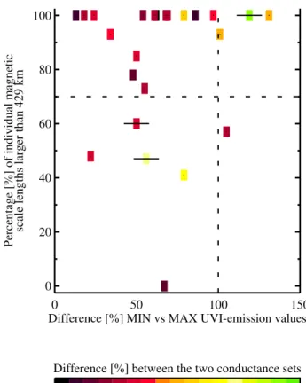
In Fig. 11, we show the relation between the three selec-tion criteria and the differences between the two conduc-tance sets. The vertical axis gives the percentage of in-dividual magnetic scale lengths larger than 429 km, while the UVI-inhomogeneities are provided along the horizontal axis. We note that 15 of the values plotted have percent-ages larger than 70% (above the dotted horizontal line) and UVI-inhomogeneities less than 100% (left side of the dot-ted vertical line). These values are assigned relatively uni-form conditions, and the red and dark red colors filling 14 of the 15 boxes reveal differences between the two conduc-tance sets of less than±30%. The 9 remaining data points marked by crosses take place during non-uniform conditions. In general, these values give significantly larger differences, as demonstrated by the orange, yellow and green colors. We also note that a thick horizontal line goes through three of these data points during non-uniform conditions. This means that they have failed to satisfy the third selection criterion re-garding the difference between the average UVI intensity for the STARE FOV vs. a larger region of∼800 km (the PIXIE resolution).

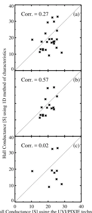
In Fig. 12, we present three scatter plots showing the cor-respondence between the two Hall conductance sets during the different ionospheric conditions. When including all 24 data points available we obtain a correlation coefficient of 0.27 (Fig. 12a). Then we plot the 15 cases of relatively uni-form ionospheric conditions, resulting in a much higher cor-relation coefficient of 0.57 (Fig. 12b). The remaining 9 data points represents non-uniform conditions. These are plotted in Fig. 12c, and the correlation coefficient drops to 0.02.

5 Conclusion

The ionospheric conductances have been derived and com-pared for three periods with substorm activity in 1998, using remote sensing of UV- and X-ray emissions (Sect. 2.1) and

0 50 100 150

Difference [%] MIN vs MAX UVI-emission values 0

20 40 60 80 100

Percentage [%] of individual magnetic

scale lengths larger than 429 km

Difference [%] between the two conductance sets

0 10 20 30 40 50 60 70 80

Fig. 11. The correspondence between percentage of individual magnetic scale lengths larger than 429 km (vertical axis), UVI-inhomogeneities (horizontal axis), and the differences between the two conductance sets (color bar). The data points assigned non-uniform conditions are marked by crosses. To fulfill the first two selection criteria, the data points must be above the dotted horizon-tal line at 70% (selection criterion No. 1) and the left side of the dotted vertical line at 100% (selection criterion No. 2). The thick horizontal lines through three of the boxes indicate the data points which do not fulfill selection criterion No. 3.

0 10 20 30 40

Hall Conductance [S] using the UVI/PIXIE technqiue 0

10 20 30 40

Hall Conductance [S] using 1D method of characteristics

0 10 20 30 40

(a)

(b)

(c)

Corr. = 0.27

Corr. = 0.57

Corr. = 0.02

✁

Fig. 12.Hall conductances6Hderived using the UVI/PIXIE tech-nique (horizontal axis) and the 1-D method of characteristics

(ver-tical axis) during(a)all conditions (24 data points),(b)relatively

uniform conditions (15 data points), and(c)non-uniform conditions

(9 data points). The dotted line having a proportionality factor of 1.0 is drawn to indicate the locations of the Hall conductance values in cases where the two data sets provide the same output.

As discussed in Sect. 1, the ionospheric conductances can be estimated using many different techniques. The reliability of the methods used in this study, involving remote sensing of UV- and X-ray emissions (Sect. 2.1) and 1-D method of characteristics (Sect. 2.2), depends on several assumptions and limitations. Our database is further restricted to 24 data points, meaning that we must be cautious when interpreting the results. Despite the limited statistics we nevertheless find

that the relation between the conductance sets is significantly improved when only including cases with relatively uniform conditions. As discussed in Sect. 2.1, studies by Germany et al. (2001) and Østgaard et al. (2001) indicate that the energy characteristics derived from UVI and PIXIE measurements, most important for the conductance calculations, are fairly reliable. This suggests that the estimated conductances us-ing Polar satellite data provide a meanus-ingful representation of the actual conductivities. The same conclusion can be made for the method of characteristics, according to inves-tigations by Amm (1995) and Amm et al. (2003). The fairly good agreement seen in Fig. 12b supports the two very dif-ferent techniques used and puts greater confidence in the two methods.

As explained in Sect. 1, it is not self-evident that simple averaging of the mesoscale results (1-D method of charac-teristics) allows for a continuous transition to the large-scale results (the UVI/PIXIE technique). By regarding the two sets of conductances as results of stochastical processes that oper-ate on different scales, a number of different situations can be imagined where averaging would not work. The correlation coefficient between the two conductance sets of 0.57 found in this study during relatively uniform conditions is not impres-sive, but still indicates that a reasonable agreement between the two methods giving large-scale and mesoscale conduc-tances can be reached. Therefore, it makes sense to study the ionospheric electrodynamics combining data with large spatial and temporal differences in the scales of the measure-ments. The lack of correspondence during non-uniform con-ditions also demonstrates the limitations of the two proce-dures, suggesting that the methods are less reliable when the local ionospheric region is in a highly turbulent state.

Acknowledgements. This study was supported by the Research

Council of Norway (NFR). The work of O. A. was supported by the Academy of Finland. The work of G. A. Germany was sup-ported by Subaward SA3527 from the University of California in Berkeley and by NASA AISRP Grant NAG5-1074. A. A. thanks A. D. Richmond for useful discussions on collision frequencies.

Topical Editor M. Lester thanks J. Watermann and another ref-eree for their help in evaluating this paper.

References

Aksnes, A., Stadsnes, J., Bjordal, J., Østgaard, N., Vondrak, R. R., Detrick, D. L., Rosenberg, T. J., Germany, G. A., and Chenette, D.: Instantaneous ionospheric global conductance maps during an isolated substorm, Ann. Geophys., 20, 1181, 2002,

SRef-ID: 1432-0576/ag/2002-20-1181.

Aksnes, A., Stadsnes, J., Lu, G., Østgaard, N., Vondrak, R. R., De-trick, D. L., Rosenberg, T. J., Germany, G. A., and Schulz, M.: Effects of energetic electrons on the electrodynamics in the iono-sphere, Ann. Geophys., 22, 475, 2004,

SRef-ID: 1432-0576/ag/2004-22-475.

Amm, O.: Method of characteristics in spherical geometry applied to a Harang-discontinuity situation, Ann. Geophys., 16, 413, 1998,

SRef-ID: 1432-0576/ag/1998-16-413.

Amm, O., Aikio, A., Bosqued, J. -M., Dunlop, M., Fazakerley, A., Janhunen, P., Kauristie, K., Lester, M., Sillanp¨a¨a, I., Tay-lor, M. G. G. T., Vontrat-Reberac, A., Mursula, K., and Andr´e, M.: Mesoscale structure of a morning sector ionospheric shear flow region determined by conjugate Cluster II and MIRACLE ground-based observations, Ann. Geophys., 21, 1737, 2003,

SRef-ID: 1432-0576/ag/2003-21-1737.

Banks, P. M. and Doupnik, J. R.: A review of auroral zone electro-dynamics deduced from incoherent scatter radar observations, J. Atmos. Terr. Phys., 37, 951, 1975.

Basu, B. and Jasperse, J. R.: Linear transport theory of auroral pro-ton precipitation: A comparison with observations, J. Geophys. Res., 92, 5920, 1987.

Baumjohann, W., Pellinen, R. J., Opgenoorth, H. J., and Nielsen, E.: Joint two-dimensional observations of ground magnetic and ionospheric electric fields associated with auroral zone currents: current system associated with local auroral break-ups, Planet. Space Sci., 29, 431, 1981.

Bostrøm, R.: A model of the auroral electrojets, J. Geophys. Res., 69, 4983, 1964.

Brekke, A.: Physics of the Upper Polar Atmosphere, John Wiley and Sons Ltd., Chichester, England, 1997.

Brekke, A., Doupnik, J. R., and Banks, P. M.: Incoherent scatter measurements of E region conductivities and currents in the au-roral zone, J. Geophys. Res., 79, 3773, 1974.

Brekke, A., Hall, C., and Hansen, T. L.: Auroral ionospheric con-ductances during disturbed conditions, Ann. Geophys., 7, 269, 1989.

Buchert, S., Baumjohann, W., Haerendel, G., La Hoz, C., and L¨uhr, H.: Magnetometer and incoherent scatter observations of an in-tense Ps 6 pulsation event, J. Atmos. Terr. Phys., 50, 357, 1988. Christakos, G.: Random Field Models in Earth Sciences, Academic

Press, San Diego, USA, 1992.

Davies, J. A. and Lester, M.: The relationship between electric fields, conductances and currents in the high-latitude ionosphere: a statistical study using EISCAT data, Ann. Geophys., 17, 43, 1999,

SRef-ID: 1432-0576/ag/1999-17-43.

de la Beaujardi`ere, O., Vondrak, R., Heelis, R., Hanson, W., and Hoffman, R.: Auroral arc electrodynamic parameters measured by AE-C and the Chatanika radar, J. Geophys. Res., 86, 4671, 1981.

Doe, R. A., Kelly, J. D., Lummerzheim, D., Parks, G. K., Brit-tnacher, M. J., Germany, G. A., and Spann, J.: Initial comparison of POLAR UVI and Sondrestrom IS radar estimates for auroral electron energy flux, Geophys. Res. Lett., 24, 999, 1997. Duschek, A. and Hochrainer, A.: Tensorrechnung in analytischer

darstellung II: Tensoranalysis, Springer-Verlag, New York, 1961. Dymond, K. F., Budzien, S. A., and Thonnard, S. E.: Electron den-sities determined by the HIRAAS experiment and comparisons with ionosonde measurements, Geophys. Res. Lett., 28, 927, 2001.

Fukushima, N.: Generalized theorem for no ground magnetic ef-fect of vertical currents connected with Pedersen currents in the uniform-conductivity ionosphere, Rep. Ionos. Space Res., Japan, 30, 35, 1976.

Gagnepain, J., Crochet, M., and Richmond, A. D.: Comparisoon of equatiorial electrojet models, J. Atmos. Terr. Phys., 39, 1119,

1977.

Germany, G. A., Torr, M. R., Richards, P. G., and Torr, D. G.: The dependence of modeled OI 1356 and N2 LBH auroral emissions on the neutral atmosphere, J. Geophys. Res., 95, 7725, 1990. Germany, G. A., Parks, G. K., Brittnacher, M., Cumnock, J.,

Lum-merzheim, D., Spann, J. F., Chen, L., Richards, P. G., and Rich, F. J.: Remote determination of auroral energy characteristics dur-ing substorm activity, Geophys. Res. Lett., 24, 995, 1997. Germany, G. A., Parks, G. K., Brittnacher, M., Spann, J. F.,

Cum-nock, J., Lummerzheim, D., Rich, F. J., and Richards, P. G.: En-ergy characterization of a dynamic auroral event using GGS UVI images, in Geospace Mass and Energy Flow: Results from the International Solar-Terrestrial Physics Program, edited by J. L. Horwitz, D. L. Gallagher, and W. K. Peterson, 143, AGU, 104, Washington, D.C., 1998a.

Germany, G. A., Spann, J. F., Parks, G. K., Brittnacher, M., Elsen, R., Chen, L., Lummerzheim, D., and Rees, M.: Auroral obser-vations from the Polar Ultraviolet Imager (UVI), in Geospace Mass and Energy Flow: Results from the International Solar-Terrestrial Physics Program, edited by J. L. Horwitz, D. L. Gal-lagher, and W. K. Peterson, 149, AGU, 104, Washington, D.C., 1998b.

Germany, G. A., Lummerzheim, D., and Richards, P. G.: Impact of model differences on quantitative analysis of FUV auroral emissions: Total ionization cross sections, J. Geophys. Res., 106, 12 837, 2001.

Gonzalez, W. D., Joselyn, J. A., Kamide, Y., Kroehl, H., Rostoker, G., Tsurutani, B. T., and Vasyliunas, V. M.: What is a geomag-netic storm?, J. Geophys. Res., 99, 5771, 1994.

Imhof, W. L., Spear, K. A., Hamilton, J. W., Higgins, B. R., Mur-phy, M. J., Pronko, J. G., Vondrak, R. R., McKenzie, D. L., Rice, C. J., Gorney, D. J., Roux, D. A., Williams, R. L., Stein, J. A., Bjordal, J., Stadsnes, J., Njøten, K., Rosenberg, T. J., Lutz, L., and Detrick, D. L.: The Polar Ionospheric X-ray Imaging Exper-iment (PIXIE), Space Sci. Rev., 71, 385, 1995.

Inhester, B., Untiedt, J., Segatz, M., and K¨urschner, M.: Direct de-termination of the local ionospheric Hall conductance distribu-tion from two-dimensional electric and magnetic field data, J. Geophys. Res., 97, 4073, 1992.

Itikawa, Y.: Effective collision frequency of electrons in atmo-spheric gases, Planet. Space Sci., 19, 993, 1971.

Kamide, Y. and Vickrey, J. F.: Relative contribution of ionospheric conductivity and electric field to the auroral electrojets, J. Geo-phys. Res., 88, 7989, 1983.

Kamide, Y., Craven, J. D., Frank, L. A., Ahn, B. -H., and Aka-sofu, S. -I.: Modeling substorm current systems using conduc-tivity distributions inferred from DE auroral images, J. Geophys. Res., 91, 11 235 1986.

Krall, N. A. and Trivelpiece, A. W.: Principles of Plasma Physics, McGraw-Hill, New York, USA, 1973.

Lorence, L. J., CEPXS/ONELD Version 2.0: A discrete ordinates code package for general one-dimensional coupled electron-photon transport, IEES Trans. Nucl. Sci, 39, 1031, 1992. L¨uhr, H., Aylward, A., Bucher, S. C., Pajunp¨a¨a, A., Pajunp¨a¨a, K.,

Holmboe, T., and Zalewski, S. M.: Westward moving dynamic substorm features observed with the IMAGE magnetometer net-work and other ground-based instruments, Ann. Geophys., 16, 425, 1998,

SRef-ID: 1432-0576/ag/1998-16-425.

Marklund, G., Sandahl, I., and Opgenoorth, H.: A study of the dynamics of a discrete auroral arc, Planet. Space Sci., 30, 179, 1982.

Mason, E. A.: Estimated ion mobilities for some air constituents, Planet. Space Sci., 18, 137, 1970.

Mersmann, U., Baumjohann, W., K¨uppers, F., and Lange, K.: Anal-ysis of an eastward electrojet by means of upward continuation of ground-based magnetometer data, J. Geophys., 45, 281, 1979. Olsson, A., Persson, M. A. L., Opgenoorth, H. J., and Kirkwood, S.: Particle precipitation in auroral breakups and westward traveling surges, J. Geophys. Res., 101, 24 661, 1996.

Opgenoorth, H. J., Pellinen, R. J., Baumjohann, W., Nielsen, E., Marklund, G., and Eliasson, L.: Three-dimensional current flow and particle precipitation in a westward travelling surge (ob-served during the barium-GEOS rocket experiment), J. Geophys. Sci., 88, 3138, 1983.

Østgaard, N., Stadsnes, J., Bjordal, J., Vondrak, R. R., Cummer, S. A., Chenette, D., Schulz, M., and Pronko, J.: Cause of the localized maximum of X-ray emission in the morning sector: A comparison with electron measurements, J. Geophys. Res., 105, 20 869, 2000.

Østgaard, N., Stadsnes, J., Bjordal, J., Germany, G. A., Vondrak, R. R., Parks, G. K., Cummer, S. A., Chenette, D., and Pronko, J.: Auroral electron distributions derived from combined UV and X-ray emissions, J. Geophys. Res., 106, 26 081, 2001.

Østgaard, N., Germany, G. A., Stadsnes, J., and Vondrak, R. R.: En-ergy analysis of substorms based on remote sensing techniques, solar wind measurements and geomagnetic indices, J. Geophys. Res., 107, 1233, 2002.

Pesnell, W. D., Omidvar, K., and Hoegy, W. R.: Momentum

trans-fer collision frequency of O+−O, Geophys. Res. Lett., 20, 1343,

1993.

Pulkkinen, A., Amm, O., and Viljanen, A.: and BEAR working group, Ionospheric equivalent current distributions determined with the method of spherical elementary current systems, J. Geo-phys. Res., 108, 1053, doi:10.1029/2001JA005085, 2003. Rees, M. H.: Auroral ionization and excitation by incident energetic

electrons, Planet. Space. Sci., 11, 1209, 1963.

Rees, M. H., Lummerzheim, D., Roble, R. G., Winningham, J. D., Craven, J. D., and Frank, L. A.: Auroral energy deposition rate, characteristic electron energy, and ionospheric parameters de-rived from Dynamics Explorer 1 images, J. Geophys. Res., 93, 12 841, 1988.

Robinson, R. M. and Vondrak, R. R.: Measurements of E region ionization and conductivity produced by solar illumination at high latitudes, J. Geophys. Res., 89, 3951, 1984.

Robinson, R. M. and Vondrak, R. R., Validation of techniques for space based remote sensing of auroral precipitation and its iono-spheric effects, Space Sci. Rev., 69, 331, 1994.

Robinson, R. M., Vondrak, R. R., Miller, K., Dabbs, T., and Hardy, D.: On calculating ionospheric conductances from the flux and energy of precipitating electrons, J. Geophys. Res., 92, 2565, 1987.

Schlegel, K.: Auroral zone E-region conductivities during solar minimum derived from EISCAT data, Ann. Geophys., 6, 129, 1988.

Senior, C.: Solar and particle contributions to auroral height-integrated conductivities from EISCAT data: a statistical study, Ann. Geophys., 9, 449, 1991.

Sillanp¨a¨a, I.: One-dimensional method of characteristics to deter-mine ionospheric conductances and currents, unpublished Grad-uate Thesis, Helsinki, Finland, 2002.

Torr, M. R., Torr, D. G., Zukic, M., Johnson, R. B., Ajello, J., Banks, P., Clark, K., Cole, K., Keffer, C., Parks, G., Tsurutani, B., and Spann, J.: A far ultaviolet imager for the international solar-terrestrial physics mission, Space Sci. Rev., 71, 329, 1995. Untiedt, J. and Baumjohann, W.: Studies of polar current sys-tems using the IMS scandinavian magnetometer array, Space Sci. Rev., 63, 245, 1993.

Vasyliunas, V. M.: Mathematical models of magnetospheric con-vection and its coupling to the ionosphere, in Particles and Fields in the Magnetosphere, edited by B. M. McCormac, 60, D. Reidel, Hinghamn, Mass., 1970.

Viehland, L. A. and Mason, E. A.: Transport Properties of Gaseous Ions Over a Wide Energy Range – Part IV, Atomic Data and Nu-clear Data Tables, 60, 37, 1995.

Vondrak, R. and Robinson, R., Inference of high-latitude ionization and conductivity from AE-C measurements of auroral electron fluxes, J. Geophys. Res., 90, 7505, 1985.

Vondrak, R. R. and Baron, M. J.: Radar measurements of the latitu-dinal variation of auroral ionization, Radio Sci., 11, 939, 1976. Vondrak, R. R., Robinson, R. M., Mizera, P. F., and Gorney, D.

J.: X-ray spectrophotometric remote sensing of diffuse auroral ionization, Radio Sci., 23, 537, 1988.

Watermann, J., de la Beaujardi`ere, O., and Rich, F. J.: Comparison of ionospheric electrical conductances inferred from coincident radar and spacecraft measurements and photoionization models, J. Atmos. Terres. Phys., 55, 1513, 1993.