Dynamic analysis and pattern visualization of forest fires.

(1)

Dynamic Analysis and Pattern Visualization of Forest

Fires

Anto´nio M. Lopes1*, J. A. Tenreiro Machado2

1Institute of Mechanical Engineering, Faculty of Engineering, University of Porto, Porto, Portugal,2Institute of Engineering, Polytechnic of Porto, Porto, Portugal

Abstract

This paper analyses forest fires in the perspective of dynamical systems. Forest fires exhibit complex correlations in size, space and time, revealing features often present in complex systems, such as the absence of a characteristic length-scale, or the emergence of long range correlations and persistent memory. This study addresses a public domain forest fires catalogue, containing information of events for Portugal, during the period from 1980 up to 2012. The data is analysed in an annual basis, modelling the occurrences as sequences of Dirac impulses with amplitude proportional to the burnt area. First, we consider mutual information to correlate annual patterns. We use visualization trees, generated by hierarchical clustering algorithms, in order to compare and to extract relationships among the data. Second, we adopt the Multidimensional Scaling (MDS) visualization tool. MDS generates maps where each object corresponds to a point. Objects that are perceived to be similar to each other are placed on the map forming clusters. The results are analysed in order to extract relationships among the data and to identify forest fire patterns.

Citation:Lopes AM, Tenreiro Machado JA (2014) Dynamic Analysis and Pattern Visualization of Forest Fires. PLoS ONE 9(8): e105465. doi:10.1371/journal.pone. 0105465

Editor:Jesus Gomez-Gardenes, Universidad de Zarazoga, Spain

ReceivedApril 21, 2014;AcceptedJuly 11, 2014;PublishedAugust 19, 2014

Copyright:ß2014 Lopes, Tenreiro Machado. This is an open-access article distributed under the terms of the Creative Commons Attribution License, which permits unrestricted use, distribution, and reproduction in any medium, provided the original author and source are credited.

Data Availability:The authors confirm that all data underlying the findings are fully available without restriction. The data used in our paper is held by the Portuguese Institute of Nature and Forest Conservation (Instituto da Conservac¸a˜o da Natureza e das Florestas - NCF) and is available for download at http://www. icnf.pt/portal/florestas/dfci/inc/estatisticas.

Funding:The authors have no support or funding to report.

Competing Interests:The authors have declared that no competing interests exist. * Email: aml@fe.up.pt

Introduction

Forest fires are a major concern in many countries, like United States, Australia, Russia, Brazil, China and Mediterranean Basin European regions [1–3]. Every year forest fires consume vast areas of vegetation, compromising ecosystems and contributing to the carbon dioxide emissions that are changing Earth’s climate [4–5]. Besides the long-term economic implications associated to the climate change, forest fires have direct impact upon economy due to the destruction of public and private property and infrastruc-tures [6]. Fires are mainly caused by natural factors, human negligence, or even human intent. Fire propagation and burnt area depend on many natural factors and conditions, not only on the terrain orography and the type of vegetation, but also on the efficacy of detection and suppression strategies. Moreover, fires caused by incendiaries contribute to increase the complexity of the phenomena. Understanding the underlying patterns of forest fires in terms of their size and spatiotemporal distributions may help the decision makers to take preventive measures beforehand, identi-fying possible hazards and deciding strategies for fire prevention, detection and suppression [7–8].

Forest fires have been studied using classical statistical tools. However, those methods reveal limitations, both in capturing all characteristics underneath forest fires dynamics, and the evolution along years [9]. Forest fires dynamics exhibits correlations in size, space and time. Size-frequency distributions unveil long range memory, which is typical in complex systems. Correlation between data is characterized by self-similarity and absence of

character-istic length-scale, meaning that forest fires exhibit power-law (PL) behaviour [10–13].

Several studies have been published during the last years about this topic [14–17]. In references [18–19] it is shown that forest fires exhibit PL frequency-size relationship over many orders of magnitude and that such behaviour seems consistent with the self-organized criticality arising in complex systems. The most important practical implication of such results is that the frequency-size distribution of small and medium fires can be used to quantify the risk of large fires [19]. Nevertheless, some authors [15] suggest that a simple PL distribution of sizes may be too simple to describe the distributions of forest fires over their full range.

In reference [20] the time dynamics of forest fires is investigated and it is shown that forest fires exhibit time-clustering phenomena. More recently, the fractality of the forest fires was addressed in [21] using spatial and temporal fractal tools. The authors prove that these phenomena exhibit space–time clustering behaviour.

(2)

extract relationships among the data. Finally, we propose an amplitude-space embedding technique that produces a clear fire pattern classification.

Characterization of the Dataset

Data from forest fires is available online at the Portuguese Institute of Nature and Forest Conservation (INCF), http://www. icnf.pt/portal/florestas/dfci/inc/estatisticas, and the catalogue contains events since 1980 up to 2012. Ignitions might have

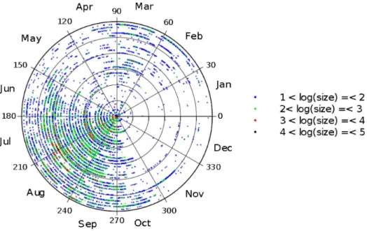
different sources, as natural causes, human negligence or human intentionality, among others. The data analysed in this paper was retrieved in December, 2013. Each record contains information about the events date, time (with one minute resolution), geographic location and size (in terms of burnt area). We decided to discard small size events, as those are prone to measurement errors, by adopting a cutoff threshold value ofAmin= 10 hectares. Fig. 1 illustrates the temporal evolution and size of the events occurred in Portugal, during 1980–2012 and meeting the cutoff threshold criterion. We tackle the concept of ‘circular time’ (since

Figure 1. Temporal evolution and size (in log units) of forest fires registered in Portugal in the time period 1980–2012, with burnt area larger thanAmin= 10 ha.Each (r,h) point represents the time of the event and the color represents the size.

doi:10.1371/journal.pone.0105465.g001

Figure 2. Evolution of burnt area per year and number of occurrences registered in Portugal in the time period 1980–2012 (are considered events with burnt area larger thanAmin= 10 ha).

(3)

there is a kind of one-year periodicity, with December close to January and not the opposite, as a Cartesian scale implicitly assumes). The (circular) time scale evolves along an Archimedean spiral, with origin at the center of the circumferences, given by:

h~2p: t Tzi

ð1Þ

r~pzq:h ð2Þ

where (r,h) denotes the radius and angle coordinates, respectively,

i= 0, …, 32, represents the year andp=q= 1. The burnt area is expressed in logarithmic units and is related to the color of the marks. We can note two annual cycles: the first is weaker and includes the months of February and March; the second is stronger and is due to the major incidence of fires during summer [22].

In Fig. 2 we depict the evolution of the burnt area per year and number of occurrences versus year. It is visible the increasing number of events as well as the strong activity verified around the middle of the decade 2000–2009. Nevertheless, the charts reveal a large volatility and pose difficulties to capture some trend. We observe minimal values for years 1983, 1988, …, 2008, and maximum values for 2003 and 2005, but no straightforward method to correlate data points. Fig. 3 represents the comple-mentary cumulative distributions of the events size and the time interval between consecutive events.

The results shown above illustrate through simple statistics the increasing importance of understanding the behavior of forest fires and characterizing the spatiotemporal distributions unveiled by such a complex phenomenon. For that purpose, in the next sections we adopt several complementary mathematical tools.

Mutual Information Analysis

In this section we adopt the mutual information to correlate forest fires annual patterns. First we compute the mutual information, based on events size (i.e., burnt area), for each pair of years in the time period 1980–2012. Second, we use a hierarchical clustering algorithm to find relationships among the

data. Visualization trees are used to highlight the interpretation of the results.

Mutual Information

The mutual information is a measure of the statistical dependence between two random variables, giving the amount of information that one variable ‘‘contains’’ about the other. IfXi

and Xj are two discrete random variables, then the mutual

information,I(Xi,Xj), is given by:

Figure 4. Contour map of the mutual information, IN(Xi, Xj),

between occurrences registered in Portugal during 1980–2012.

The cutoff threshold valueAmin= 10 ha is adopted.

Figure 5. Tree representing mutual information, IN(Xi, Xj),

between occurrences registered in Portugal during 1980– 2012.The cutoff threshold valueAmin= 10 ha is adopted.

Figure 3. Complimentary cumulative distribution of events size and time interval (in minutes) between consecutive events, corresponding to occurrences registered in Portugal in the time period 1980–2012, with burnt area larger than

Amin= 10 ha.

(4)

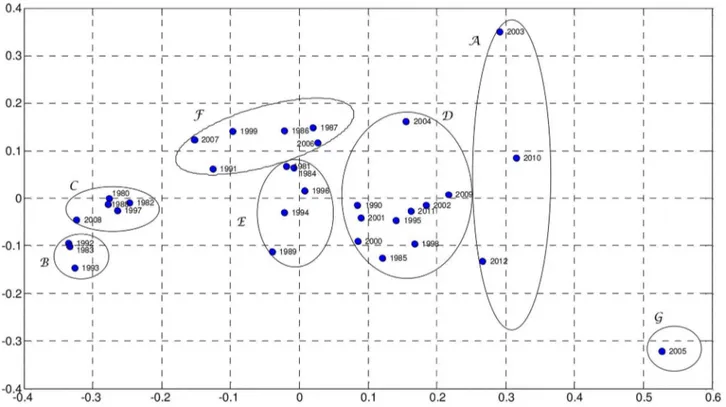
Figure 6. MDS map based on matrix D, for visualization space with dimensionm= 2.

Figure 7. MDS map based on matrix D, for visualization space with dimensionm= 3.

(5)

I(Xi,Xj)~X

xj[Xj

X

xi[Xi

p(xi,xj):log

p(xi,xj) p(xi):p(xj)

ð3Þ

wherep(xi, xj) is the joint probability distribution function of (Xi,

Xj), andp(xi) andp(xj) are the marginal probability distribution functions ofXiandXj, respectively.

The concept of mutual information comes from the information theory [23] and has been adopted in the study of complex systems from diverse fields, namely in experimental time series analysis, in

DNA and symbol sequencing and in providing a theoretical basis for the notion of complexity [24–30].

In this section, instead of expression (3), we use the normalized mutual information,IN(Xi,Xj), given by [31]:

IN(Xi,Xj)~I(Xi,Xj)

H(Xi,Xj) ð4Þ

whereH(Xi,Xj) represents the joint entropy betweenXiandXj:

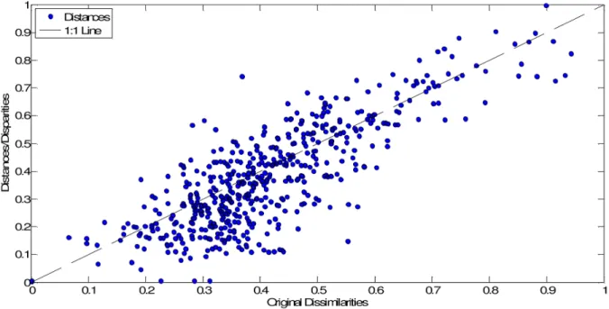
Figure 8. Shepard plot of the MDS map based on matrix D, for visualization space with dimensionm= 2.

Figure 9. Shepard plot of the MDS map based on matrix D, for visualization space with dimensionm= 3.

(6)

H(Xi,Xj)~{X

xj[_Xj

X

xi[_Xi

p(xi,xj):logp(xi,xj)

ð5Þ

The normalized mutual informationIN(Xi,Xj)M_{[0, 1] simplifies}

comparison across different conditions and improves sensitivity. Forest fires are analysed in an annual basis. For each year,i= 0, …, 32, in the period 1980–2012 the events are represented by:

xi(t)~X

T

k~1

Akd(t{tk), i~0, ,32 ð6Þ

leading to 33 one-year length time series. This means that the events are modelled as Dirac impulses, whereAk represents fire size (i.e., burnt area), tk is the instant of occurrence (with one minute resolution),trepresents time andTdenotes the time period of one year.

The signalsxi(t) are then normalized according to (7):

~ x

xi(t)~xi(t)

{m

s ð7Þ

wheremandsrepresent the mean and standard deviation values of all events listed during 1980–2012, with magnitude larger than

Amin= 10 ha. The mutual information is calculated to correlate events occurred in different years of the analysed time period.

Fig. 4 depicts in a contour map the mutual information,IN(Xi, Xj), between every pair of yearsi,j= 0, …, 32. The probabilities

for calculating the mutual information are estimated from the histograms of amplitudes Ak, constructed considering 476 bins,

each one having width equal to 0.1 ha. To facilitate the comparison the cases i=j (i.e., those with maximum value of mutual information) are removed from the graph.

The map reveals strong correlations between certain years, corresponding to higher values of mutual information. This is well noted for the years a = {2003, 1983}, b = {2003, 1993}, c = {2005, 1980}, d = {2005, 1983}, e = {2005, 1988}, f = {2005, 1993}, g = {2008, 2005} and h = {2010, 1983}. Nevertheless, the analysis is not totally assertive and requires multiple comparisons.

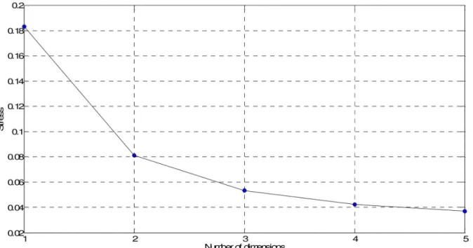
Figure 10. Stress plot for the MDS based on matrix D.

Figure 11. Bidimensional histogram of forest fires versus latitude and longitude, in Portugal, for year 2010.

(7)

Hierarchical clustering

Having in mind an efficient method to visualize and to compare results, a hierarchical clustering algorithm is adopted, based on the mutual information,IN(Xi,Xj), between pairs of objects.

The goal of hierarchical clustering is to build a hierarchy of clusters, in such a way that objects in the same cluster are, in some sense, similar to each other [30,32–33]. Based on a measure of dissimilarity between clusters, those are combined (or, alternative-ly, split) for agglomerative (or, alternativealternative-ly, divisive) clustering. This is achieved by using an appropriate metric, quantifying the distance between pairs of objects, and a linkage criterion, defining the dissimilarity between clusters as a function of the pairwise distances between objects. The results of hierarchical clustering are presented in a phylogenetic tree adopting the successive (agglom-erative) clustering and average-linkage method (Fig. 5). The software PHYLIP was used for generating both graphs (http:// evolution.genetics.washington.edu/phylip.html).

Fig. 5 unveils groups of objects (years) in such a way that objects in the same group (cluster) are more similar to each other than to

those in other groups. For example, we can easily identify clusters composed by years A = {2003, 2010, 2012}, B = {1983, 1992, 1993} and C = {1980, 1982, 1988, 1997, 2008,}. On the contrary, year G = {2005} is far aside, meaning that it is different from all the rest. Both representations of Fig. 4 and Fig. 5 can be used to visualise and to compare the events, in an annual basis. Fig. 5 leads to a result easier to interpret than Fig. 4, as it identifies groups of objects that are similar.

MDS Analysis and Visualization

In this section we adopt the MDS tools to handle information and the relationships embedded into the data.

MDS is a statistical technique for visualizing data that can reveal similarities between objects. The algorithm requires the definition of a similarity measure (or, inversely, of a distance) and the construction of as6s symmetric matrix Dof similarities (or distances) between each pair ofsobjects. MDS assigns a point to each object in am-dimensional space and arranges the set in order to reproduce the observed similarities. A shorter (larger) distance between two points means that the corresponding objects are more similar (distinct). For m= 2 or m= 3 dimensions the resulting locations may be displayed in a ‘‘map’’ that can be visualized [34– 39].

In our case, we obtainD(33633 dimensional) by means of the mutual information (4). Fig. 6 and Fig. 7 show the MDS maps for

m= 2 and m= 3, respectively. The Shepard and the stress plots assess the quality of the MDS maps. The Shepard diagrams (Fig. 8 and Fig. 9) show an acceptable distribution of points around the 45 degree line, which means a good fit of the distances to the dissimilarities. On the other hand, the stress plot reveals that a three dimensional space describes adequately the data (Fig. 10). This can be concluded by observing the stress line, which diminishes strongly until the dimensionality is two, moderately towards dimensionality three and weakly from then on. Often, the maximum curvature point of the stress line is adopted as the criterion for deciding the dimensionality of the MDS map.

The MDS maps of Fig. 6 and Fig. 7 confirm the groups previously identified by the hierarchical clustering and, conse-quently, the relationships between the corresponding yearly patterns. Comparing Fig. 5 with Fig. 6 and Fig. 7, we conclude that all allow an easy interpretation of the results. The MDS maps, in particular the 3D plot, are more intuitive than the phylogenetic

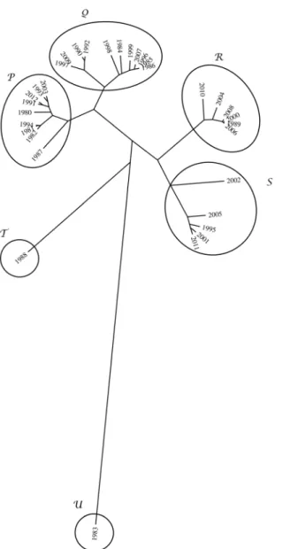
Figure 12. Tree comparing the 33 bidimensional histograms based on indexdij.

Figure 13. Entropy, Si, versus year, during the time period

1980–2012.

(8)

tree. Moreover, most software for MDS analysis allows the user to rotate and visualise the maps from different perspectives, easing the identification of clusters. This is useful especially when dealing with large amounts of data.

Forest Fires Spatial Patterns

In this section we study forest fires in a complementary line of thought, namely by considering spatial information. First, we divide the geographic territory under study (i.e., 36.95u# lat #

42.15u;29.50u#lon#26.19u), using aM6N(M= 30,N= 15) rectangular grid, and we determine the 33 bidimensional histograms of relative frequencies for all years in the period 1980–2012. Second, for characterizing the histograms, we calculate the Shannon entropy,Si, given by:

Si~{X

M

m~1

XN

n~1

pi(m,n):log½pi(m,n), i~0, ,32 ð8Þ

where the probabilitiespi(m,n) are approximated by the relative frequencies.

In Fig. 11, for example, we depict the bidimensional histogram for year 2010. The corresponding entropy isSi= 4.08 (i= 30).

For histogram comparison we calculate a M6N symmetric matrixD= [dij], where

dij~DSi{SjD, i,j~0, ,32 ð9Þ

The results are visualized in the phylogenetic tree of Fig. 12. We can observe six clusters: P = {1980, 1981, 1982, 1987, 1991, 1993, 1994, 2003, 2012}; Q = {1984, 1985, 1986, 1990, 1992, 1996, 1997, 1998, 1999, 2007, 2009}; R = {1989, 2000, 2004, 2006, 2008, 2010}; S = {1995, 2001, 2002, 2005, 2011}; T = {1983} and U = {1988}.

The evolution ofSiversus year is represented in Fig. 13, where the clusters shown in Fig. 12 are identified. In this chart is clear a large volatility and apparently some increase of entropy along time.

In a more global perspective, we verify that amplitude and space data lead to distinct observations. The conclusions are ‘decoupled’ and reveal that both directions must be explored, with more data, in order to include all information in a global tool of analysis.

In this line of though, we embed amplitude and space data into a single graph by adding to the bidimensional MDS plot of Fig. 6 a vertical axis representing the Shannon entropy (Fig. 14).

We note that only two years, Y = {1983} and Z = {2005}, have now a clearly distinct separation from the main cluster, X. In Fig. 13 we observed them to be located at near extreme values, but, as mentioned, it is difficult to get idea due to large volatility. The embedding of amplitude-space techniques produced a clear classification pattern.

Conclusions

We analysed forest fires from the perspective of dynamical systems. Data from a public domain forest fires catalogue, containing information of events for Portugal, during the period 1980–2012, was studied in an annual basis. Mutual information to correlate annual patterns was considered. Phylogenetic trees generated by hierarchical clustering algorithms and MDS visualization tools were used to compare to extract relationships among the data and to identify forest fire patterns. Those tools allow different perspectives over forest fires that may be used to better understand the dynamics emerging in the plethora of phenomena that occur in forest fires.

Author Contributions

Conceived and designed the experiments: AML JTM. Performed the experiments: AML. Analyzed the data: AML JTM. Contributed reagents/

Figure 14. MDS 2D plot with the vertical axis representing Shannon entropy.

(9)

materials/analysis tools: AML JTM. Contributed to the writing of the manuscript: AML JTM.

References

1. Di Bella CM, Jobba´gy EG, Paruelo JM, Pinnock S (2006) Continental fire density patterns in South America. Global Ecology and Biogeography 15, 192– 199.

2. Bradstock RA (2008) Effects of large fires on biodiversity in south-eastern Australia: disaster or template for diversity?. International Journal of Wildland Fire 17, 809–822.

3. Hanson CT, Odion DC (2013) Is fire severity increasing in the Sierra Nevada, California, USA?. International Journal of Wildland Fire 23, 1–8.

4. Flannigan MD, Krawchuk M, de Groot W, Wotton B, Gowman L (2009) Implications of changing climate for global wildland fire. International Journal of Wildland Fire 18, 483–507.

5. Zumbrunnen T, Pezzatti GB, Mene´ndez P, Bugmann H, Bu¨rgi M, et al. (2011) Weather and human impacts on forest fires: 100 years of fire history in two climatic regions of Switzerland. Forest Ecology and Management, 261, 2188– 2199.

6. Silva FR, Gonza´lez-Caba´n A (2010) ‘SINAMI’: a tool for the economic evaluation of forest fire management programs in Mediterranean ecosystems. International journal of wildland fire, 19 927–936.

7. Zamora R, Molina-Martı´nez JR, Herrera MA, Rodrı´guez y Silva F (2010) A model for wildfire prevention planning in game resources. Ecological Modelling 221, 19–26.

8. Preisler HK, Westerling AL, Gebert KM, Munoz-Arriola F, Holmes TP (2011) Spatially explicit forecasts of large wildland fire probability and suppression costs for California. International Journal of Wildland Fire 20, 508–517.

9. Alvarado E, Sandberg DV, Pickford SG (1998) Modeling Large Forest Fires as Extreme Events. Northwest Science 72, 66–75.

10. Bak P, Chen K, Tang C (1990) A forest-fire model and some thoughts on turbulence. Physics Letters A 147, 297–300.

11. Barford P, Bestavros A, Bradley A, Crovella M (1999) Changes in Web client access patterns: characteristics and caching implications. World Wide Web 2, 15–28.

12. Baraba´si AL (2005) The origin of bursts and heavy tails in human dynamics. Nature 435, 207–211.

13. Pinto CMA, Lopes AM, Tenreiro Machado JA (2012) A review of power laws in real life phenomena. Communications in Nonlinear Science and Numerical Simulations 17, 3558–3578.

14. Ricotta C, Avena G, Marchetti M (1999) The flaming sandpile: self-organized criticality and wildfires. Ecological Modelling 119, 73–77.

15. Reed W, McKelvey K (2002) Power-law behaviour and parametric models for the size-distribution of forest fires. Ecological Modelling 150, 239–254. 16. Prentice IC, Kelley DI, Foster PN, Friedlingstein P, Harrison SP, et al. (2011)

Modeling fire and the terrestrial carbon balance. Global Biogeochemical Cycles. 25, GB3005

17. Fletcher IN, Araga˜o LE, Lima A, Shimabukuro Y, Friedlingstein P (2013) Fractal properties of forest fires in Amazonia as a basis for modelling pan-tropical burned area. Biogeosciences Discussions 10, 14141–14167. 18. Drossel B, Schwabl F (1992) Self-organized critical forest-fire model. Physical

Review Letters 69, 1629–1632.

19. Malamud B, Morein G, Turcotte D (1998) Forest Fires: An Example of Self-Organized Critical Behavior. Science 281, 1840–1842.

20. Telesca L, Amatulli G, Lasaponara R, Lovallo M, Santulli A (2005) Time-scaling properties in forest-fire sequences observed in Gargano area (southern Italy). Ecological Modelling 185, 531–544.

21. Telesca L, Amatucci G, Lasaponara R, Lovallo M, Rodrigues MJ (2007) Space– time fractal properties of the forest-fire series in central Italy. Communications in Nonlinear Science and Numerical Simulation 12, 1326–1333.

22. Marques S, Borges JG, Garcia-Gonzalo J, Moreira F, Carreiras JMB, et al. (2011) Characterization of wildfires in Portugal. European Journal of Forest Research 130, 775–784.

23. Shannon CE (1948) A Mathematical Theory of Communication. Bell System Technical Journal 27, 379–423, 623–656.

24. Herzel H, Schmitt AO, Ebeling W (1994) Finite Sample effects in Sequence Analysis. Chaos, Solitons & Fractals 4, 97–113.

25. Mori T, Kudo K, Tamagawa Y, Nakamura R, Yamakawa O, et al. (1998) Edge of chaos in rule-changing cellular automata. Physica D 116, 275–282. 26. Matsuda H (2000) Physical nature of higher-order mutual information: Intrinsic

correlations and frustration. Physical Review E 62, 3096–3102.

27. Posadas A, Hirata T, Vidal F, Correig A (2000) Spatio-temporal seismicity patterns using mutual information application to southern Iberian peninsula (Spain) earthquakes. Physics of the Earth and Planetary Interiors 122, 269–276. 28. Telesca L (2011) Tsallis-Based Nonextensive Analysis of the Southern California

Seismicity. Entropy 13, 1267–1280.

29. Mohajeri N, Gudmundsson A (2012) Entropies and Scaling Exponents of Street and Fracture Networks. Entropy 14, 800–833.

30. Tenreiro Machado JA, Lopes AM (2013) Analysis and Visualization of Seismic Data using Mutual Information. Entropy 15, 3892–3909.

31. Kvalseth TO (1987) Entropy and correlation: Some comments. IEEE Transactions on Systems, Man and Cybernetics 17, 517–519.

32. Jain A, Dubes R (1988) ‘Algorithms for Clustering Data.’ (Prentice-Hall: Englewood Cliffs, NJ).

33. Johnson SC (1996) Hierarchical clustering schemes. Psychometrika 32, 241–54. 34. Shepard R (1962) The analysis of proximities: multidimensional scaling with an

unknown distance function. Psychometrika 27, 219–246.

35. Kruskal J, Wish M (1978) ‘Multidimensional Scaling.’ (Sage Publications: Newbury Park, CA).

36. Cox T, Cox M (2001) ‘Multidimensional scaling.’ (Chapman & Hall/CRC). 37. Martinez W, Martinez A (2005) ‘Exploratory Data Analysis with MATLAB.’

(Chapman & Hall/CRC Press: UK).

38. Tzagarakis C, Jerde TA, Lewis SM, Ugurbil K, Georgopoulos AP (2009) Cerebral cortical mechanisms of copying geometrical shapes: a multidimensional scaling analysis of FMRI patterns of activation, Experimental Brain Research 194, 369–380.

39. Costa AM, Tenreiro Machado JA, Quelhas MD (2011) Histogram-based DNA analysis for the visualization of chromosome, genome and species information. Bioinformatics 27, 1207–1214.