www.atmos-chem-phys.net/7/5569/2007/ © Author(s) 2007. This work is licensed under a Creative Commons License.
Chemistry
and Physics
Emissions from forest fires near Mexico City
R. J. Yokelson1, S. P. Urbanski2, E. L. Atlas3, D. W. Toohey4, E. C. Alvarado5, J. D. Crounse6, P. O. Wennberg7, M. E. Fisher4, C. E. Wold2, T. L. Campos8, K. Adachi9,10, P. R. Buseck9,10, and W. M. Hao2
1University of Montana, Department of Chemistry, Missoula, MT 59812, USA 2USDA Forest Service, Fire Sciences Laboratory, Missoula, MT, USA
3University of Miami, Rosenstiel School of Marine and Atmospheric Science, USA 4University of Colorado, Department of Atmospheric and Oceanic Sciences, Boulder, USA 5University of Washington, College of Forest Resources, Seattle, USA
6Division of Chemistry and Chemical Engineering, California Institute of Technology, Pasadena, USA
7Divisions of Engineering and Applied Science and Geological and Planetary Science, California Institute of Technology,
Pasadena, USA
8National Center for Atmospheric Research, Boulder, CO, USA
9School of Earth and Space Exploration, Arizona State University, Tempe, AZ, USA 10Department of Chemistry and Biochemistry, Arizona State University, Tempe, AZ, USA
Received: 19 April 2007 – Published in Atmos. Chem. Phys. Discuss.: 16 May 2007 Revised: 14 August 2007 – Accepted: 27 October 2007 – Published: 9 November 2007
Abstract. The emissions of NOx(defined as NO (nitric
ox-ide) + NO2(nitrogen dioxide)) and hydrogen cyanide (HCN),
per unit amount of fuel burned, from fires in the pine forests that dominate the mountains surrounding Mexico City (MC) are about 2 times higher than normally observed for for-est burning. The ammonia (NH3) emissions are about
av-erage for forest burning. The upper limit for the mass ra-tio of NOx to volatile organic compounds (VOC) for these
MC-area mountain fires was∼0.38, which is similar to the NOx/VOC ratio in the MC urban area emissions inventory
of 0.34, but much larger than the NOx/VOC ratio for
tropi-cal forest fires in Brazil (∼0.068). The nitrogen enrichment in the fire emissions may be due to deposition of nitrogen-containing pollutants in the outflow from the MC urban area. This effect may occur worldwide wherever biomass burning coexists with large urban areas (e.g. the tropics, southeast-ern US, Los Angeles Basin). The molar emission ratio of HCN to carbon monoxide (CO) for the mountain fires was 0.012±0.007, which is 2–9 times higher than widely used literature values for biomass burning. The ambient molar ra-tio HCN/CO in the MC-area outflow is about 0.003±0.0003. Thus, if only mountain fires emit significant amounts of HCN, these fires may be contributing about 25% of the CO production in the MC-area (∼98–100 W and 19–20 N). Com-paring the PM10/CO and PM2.5/CO mass ratios in the MC
Metropolitan Area emission inventory (0.0115 and 0.0037) Correspondence to:R. J. Yokelson
to the PM1/CO mass ratio for the mountain fires (0.133) then suggests that these fires could produce as much as∼79–92% of the primary fine particle mass generated in the MC-area. Considering both the uncertainty in the HCN/CO ratios and secondary aerosol formation in the urban and fire emissions implies that about 50±30% of the “aged” fine particle mass in the March 2006 MC-area outflow could be from these fires.
1 Introduction
surround MC – usually between the hours of 10 a.m. and 6 p.m. During the January through June dry season, read-ily visible biomass burning in the surrounding mountains also occurs mainly during the afternoon. Thus, an air mass may mix with: fire emissions upwind of MC, then the MC pollutants (which may contain some urban biomass burning emissions), and then fire emissions immediately downwind of MC. The resulting plume then further evolves chemically downwind during regional transport. A key goal of MILA-GRO is to develop photochemical models that accurately re-produce the actual evolution of the MC plume measured dur-ing March 2006 research flights. For these dry season mea-surements, entrained fire emissions could affect the observed photochemical transformations. Since HCN is likely emitted mostly or exclusively by fires (Li et al., 2000), measurements of HCN emissions by fires and of HCN in the downwind plume could help quantify the biomass-burning contribution to the downwind plume.
As part of MILAGRO, an instrumented US Forest Ser-vice Twin Otter aircraft measured the emissions from 63 fires throughout south-central Mexico. This paper focuses on a “study area” ranging from 19–20 N and 98–100 W that in-cludes the MC metropolitan area and the adjacent mountains. This “box” approximates the source region relevant for air-borne measurements several hours to several days downwind of MC. The Twin Otter sampled 8 fires in this study area, of which 7 were sampled with instrumentation capable of mea-suring reactive nitrogen species. All the fires were located in the pine-dominated forests that dominate the mountains near MC. One plume from a similar MC-area fire was pro-filed by the NCAR C-130 while measuring HCN and CO and both these species were also measured regionally on board the C-130. The purpose of this paper is to present emis-sion factor and emisemis-sion ratio measurements for the pine-dominated forest fires in the MC-area mountains and a few preliminary implications of those measurements. In addition, we propose that the emissions from these fires were proba-bly impacted by the deposition of urban pollutants in the MC plume. This is likely relevant to understanding atmospheric chemistry wherever biomass burning coexists with urban ar-eas globally. Future papers will present other atmospheric chemistry measurements made on the MILAGRO research aircraft and the emission factors for the other fires sampled throughout south-central Mexico. The latter included tropi-cal deforestation fires, other forest fires, shrub and grassland fires, and agricultural waste burning.
2 Experimental details
2.1 Data acquisition
2.1.1 Airborne Fourier transform infrared spectrometer (AFTIR)
The AFTIR on the Twin Otter provided measurements of several nitrogen species and other reactive and stable trace gases present above ∼5–20 ppbv. The AFTIR had a ded-icated, halocarbon-wax, coated inlet that directed ram air through a Pyrex, multipass cell. The AFTIR was used for continuous measurements of water vapor (H2O),
car-bon dioxide (CO2), carbon monoxide (CO), and methane
(CH4); or to grab samples for signal averaging and
measure-ment of H2O, CO2, CO, nitric oxide (NO), nitrogen
diox-ide (NO2), ammonia (NH3), hydrogen cyanide (HCN), CH4,
ethene (C2H4), acetylene (C2H2), formaldehyde (HCHO),
methanol (CH3OH), acetic acid (CH3COOH), formic acid
(HCOOH), and ozone (O3). The details and the accuracy of
the AFTIR technique are described by Yokelson et al. (1999, 2003a, b).
2.1.2 Whole air sampling (WAS)
A forward facing, 25 mm i.d. stainless steel elbow sam-pled ram air into stainless steel canisters on board the Twin Otter. Two-liter canisters were shipped to the University of Miami and analyzed by gas chromatography (GC) with a flame ionization detector (FID) for CH4, and the
fol-lowing non-methane hydrocarbons: ethane, C2H4, C2H2,
propane, propene, isobutane, n-butane, t-2 butene, 1-butene, isobutene, c-2-butene, 1,3 butadiene, cyclopentane, isopen-tane, and n-penisopen-tane, with detection limits in the low pptv. CO was measured in parallel with the CH4 measurement,
but utilized GC with a Trace Analytical Reduction Gas De-tector (RGD). Starting 18 March, 800-ml canisters were also filled with the same sampling system and analyzed later at the United States Forest Service (USFS) Fire Sciences Lab-oratory by GC/FID/RGD for CO2, CO, CH4, H2, and
sev-eral C2-C3hydrocarbons. Details of the canister analysis are
given by Weinheimer et al. (1998), Flocke et al. (1999), and Hao et al. (1996). GC with mass-selective detection (MSD) measurements of higher molecular weight hydrocarbons and halocarbons will be reported elsewhere. CO and CH4were
measured with high accuracy by both the AFTIR and the cans, which facilitated coupling the data from these instru-ments.
2.1.3 Nephelometry
The large-diameter, fast-flow, WAS inlet also supplied sam-ple air for a Radiance Research Model 903 integrating neph-elometer that measuredbscat at 530 nm at 0.5 Hz;
campaign, the measurements of bscat by the
nephelome-ter were compared to gravimetric (filnephelome-ter-based) measure-ments of the mass of particles with aerodynamic diameter
<2.5 microns (PM2.5) for 14 fires in pine forest fuels burned
in the US Forest Service Missoula biomass fire simulation facility. We obtained (and applied) a linear relationship be-tweenbscatand PM2.5inµg/m3of standard temperature and
pressure air.
bscat×228 000(±11 000(2σ ))=PM2.5(µg/m3) (1)
The conversion factor is similar to the 250 000 measured by Nance et al. (1993) for smoke from Alaskan wildfires in coniferous fuels, which they showed was within±20% of the factors determined in other studies of biomass burning smoke. In addition, an earlier study in the Missoula fire lab, with fires in a larger variety of wildland fuels, found that the conversion factor of 250 000 reproduced gravimetric par-ticle mass measurements within±12% (Trent et al., 2000). We note that these conversion factors were measured in fresh smoke and are used only for fresh smoke in this work. 2.1.4 TEM analysis and co-located, fast, isokinetic particle
and CO2measurements
An isokinetic particle inlet (Jonsson et al., 1995) was used on the Twin Otter to sample fine particles with a diame-ter cut-off of a few microns. Both the measured and previ-ously published particle size distributions show that particles of diameter below 1 micron account for nearly all the fine-particle (PM2.5) mass emitted by biomass fires (Radke et al.,
1991). This inlet supplied sample air for two MPS-3 parti-cle samplers (California Measurements, Inc.) that were used to collect 182 samples over time intervals of∼1 to 10 min for analyses using transmission electron microscopy (TEM). Each sampler consists of a three-stage impactor, which col-lects particles with aerodynamic diameters of >2, 2–0.3,
<0.3µm. A CM 200 (FEI) microscope was used for sub-sequent TEM analysis at Arizona State University, which re-vealed details of the chemistry and structure of individual particles.
The same inlet also supplied a LiCor (Model #7000) mea-suring CO2 and H2O at 5 Hz and the UHSAS (Ultra High
Sensitivity Aerosol Spectrometer, Droplet Measurement Technologies) (both deployed by U. Colorado). The UHSAS provided the number of particles in each of 99 user-selectable bins for diameters between 55 and 1000 nm at 1 Hz. All three inlets were located near each other as can be seen in the photo at (https://www.umt.edu/chemistry/faculty/yokelson/ galleries/Mexico/Airborne/Aircraft/index.html). Use of a single inlet for both the UHSAS and fast CO2enabled
cou-pling the particle and trace gas data.
2.1.5 HCN and CO measurements on the C-130
The California Institute of Technology chemical ionization mass spectrometer (CIMS) measured selected product ions
on the C-130 via reaction of the reagent ion CF3O−with
an-alytes directly in air. HCN is measured by monitoring the product ion withm/z=112, which is the cluster of CF3O−
with HCN. The sensitivity is dependent on the water vapor mixing ratio. Sensitivity changes due to water vapor changes are corrected for using the dewpoint hygrometer water mea-surement from the C-130 aircraft, and a water calibration curve which has been generated though laboratory measure-ments. Non-water sensitivity changes are corrected for using in-flight standard addition calibrations of H2O2 and HNO3
(other species measured by the CIMS) and proxied to labo-ratory calibrations of HCN. The detection limit (S/N=1) for HCN for a 0.5 second integration period is better than 15 pptv for moderate to low water vapor levels (H2O mixing ratio ≤0.004) (Crounse et al., 2006).
A CO vacuum ultraviolet (UV) resonance fluorescence in-strument, similar to that of Gerbig et al. (1999), was operated on the C-130 through the National Center for Atmospheric Research and NSF. The MILAGRO data have a 3 ppbv pre-cision, 1-s resolution, and a typical accuracy of±10% for a 100 ppbv ambient mixing ratio.
2.1.6 Airborne sampling protocol
The Twin Otter and C-130 were based in Veracruz with the 4 other MILAGRO research aircraft (http://mirage-mex.acd. ucar.edu/). The Twin Otter flew 67 research hours from 4– 29 March in the approximate range 16–23 N and 88–102 W. Background air was thoroughly characterized while search-ing for fires. The nephelometer, LiCor, UHSAS, and the AFTIR were usually operated continuously in background air with similar time resolutions from 0.5 to 5 Hz. At many key locations, the MPS-3 obtained integrated samples and WAS and AFTIR acquired “grab” samples of background air. To measure the initial emissions from the fires, we sampled smoke less than several minutes old by penetrating the col-umn of smoke 150–500 m above the flame front. The LiCor, UHSAS, and nephelometer profiled their species while pen-etrating the plume. The AFTIR, MPS-3, and WAS were used to acquire “grab” samples in the smoke plumes. More than a few kilometers downwind from the source, smoke sam-ples are usually already “photochemically aged” and bet-ter for probing post-emission chemistry than estimating ini-tial emissions (Goode et al., 2000; Hobbs et al., 2003). To determine excess concentrations in the smoke-plume grab-samples, paired background grab-samples were acquired just outside the plume.
Fig. 1. The location of the MODIS hotspots and the fires sampled by MILAGRO aircraft in the study area. The land cover map in Fig. 1 is based on the 1 km2 resolution North American Seasonal Land Cover Database Version 2.0 (SLCV2.0) from the USGS Land Cover Characterization Database (http://edcsns17.cr.usgs.gov/glcc/glcc.html; Loveland et al., 2000). The original land cover categories of SLCV2.0 were aggregated to produce the simplified land cover classification used in Fig. 1. The mixed forest category consists mostly of pine mixed with other conifers or oak.
2.1.7 Ground-based fire and fuel consumption measure-ments
All but a few of the many fires observed from the MILAGRO aircraft in our MC study area were understory fires in forests dominated by pine that were located in the mountains. How-ever, overlapping the March 2006 MODIS hotspots (http: //maps.geog.umd.edu; Justice et al., 2002) with a vegetation map (Loveland et al., 2000) indicates that a sizeable frac-tion of the fires occurred in grassland or shrubland (Fig. 1). This may be partly due to the fact that fires under a forest canopy can be difficult to detect from space (Brown et al., 2006). In addition, at least two of the forest fires we actu-ally sampled (and photographed) are in non-forest areas ac-cording to multiple vegetation maps (INEGI and INE, 1998; CONABIO, 1999; Loveland et al., 2000). In any case, to ensure both airborne and ground-based sampling of a repre-sentative, well-characterized fire; a planned fire was carried out by CONAFOR (Mexican Federal Forest Service) and the Department of Ecology of the state of Morelos. Prescribed
Table 1.Locations, times, and fuel consumption for the pine-dominated forest fires sampled by the MILAGRO aircraft or ground crew in the mountains surrounding Mexico City.
time of airborne sampling
Fire Sampled by Burn Date(s) Lat (N) Long (W) start finish Coverage by cloud-free MODIS OP UMD hotspot? Fuel Consumption Burned Area Name dd/mm/yyyy dd.dddd dd.dddd hh:mm (LT) hh:mm (LT) Terra hhmm (LT) Aqua hhmm (LT) Y or N Mg total hectares 3 6-F1 TOa 06/03/2006 19.0763 99.0537 13:27 11:15 14:20 N nm nm
3 6-F2 TO, Gb 06/03/2006 19.1739 99.1903 13:32 11:15 14:20 N 61 7.7
3 6-F3 TO 06/03/2006 19.1881 99.3783 17:05 17:09 11:15 14:20 N nm nm 3 6-F4 TO 06/03/2006 19.0711 99.2283 17:14 11:15 14:20 N nm nm M6 F12 G 06/03/2006 19.3142 99.4290 none 11:15 14:20 N 85 3.7 3 9-F1 TO 09/03/2006 19.3269 99.4775 13:20 11:41 none N nm nm 3 10-F1 C-130 10/03/2006 19.6431 98.3578 17:16 10:55 13:55 N nm nm 3 17-PF TO, G 17/03/2006 19.0681 99.0616 11:58 12:42 10:55 14:00 N 145 22.2 3 17-F2 TO 17/03/2006 19.3862 98.6066 13:06 13:18 10:55 14:00 N nm nm 3 18-F2 TO, G 18/03/2006 19.3456 98.6851 15:46 16:39 11:34 none N 873 27.2 3 18-F3 G ∼17–19/03/2006 19.3174 98.6888 none Hotspot at 19.32,−98.72 (3/17 AQUA at 14:00) ∼3100 ∼300
M6 F8 G unknown 19.2252 99.3934 none N nm 6.9 Approximate Mexico City Center 19.411 99.131
aTO indicates USFS Twin Otter (see text).
bG indicates ground-based fire characterization crew (see text).
Some of the other pine-understory fires sampled by the Twin Otter were later located by the ground-based crew. The burned area was measured and the fuel consumption was measured by comparing adjacent burned and unburned areas that had similar vegetation and terrain (Table 1). In addition, forest fires that were not sampled by the MILAGRO aircraft were also located by the ground-based crew and the burned area and fuel consumption measurements obtained are also shown in Table 1.
2.2 Data processing and synthesis
Grab samples or profiles of an emission source provide ex-cess mixing ratios (1X, the mixing ratio of species “X” in the plume minus the mixing ratio of “X” in the background air). 1Xreflect the instantaneous dilution of the plume and the instrument response time. Thus, a useful, derived quan-tity is the normalized excess mixing ratio where1Xis com-pared to a simultaneously measured plume tracer such as
1CO or1CO2. A measurement of1X/1CO or1X/1CO2
made in a nascent plume (seconds to a few minutes old) is an emission ratio (ER). For any carbonaceous fuel, a set of ER to CO2 for the other major carbon emissions (i.e. CO,
CH4, a suite of non-methane organic compounds (NMOC),
particulate carbon, etc.) can be used to calculate emission factors (EF, g compound emitted/kg dry fuel burned) for all the emissions quantified from the source using the carbon mass-balance method (Yokelson et al., 1996). In this project, the carbon data needed to calculate EF was provided mostly by AFTIR measurements of CO2, CO, CH4, and NMOC and
also canister sampling of CO2, CO, CH4, and non-methane
hydrocarbons (NMHC). The particle data allowed inclusion of particle carbon in the carbon mass balance. Next we sum-marize a few details of the methods we used to synthesize the data from the various instruments on the aircraft and to calculate ER and EF.
2.2.1 Estimation of fire-average, initial emission ratios (ER) for trace gases
First we describe the computation of ER on a molar basis to CO and/or CO2for each species detected in the AFTIR and
canister grab samples. This is done for each individual fire or each group of co-located, similar fires. If there is only one grab sample of a fire (as for the 9 March fire) then the calculation is trivial and equivalent to the definition of1X
given above. For multiple grab samples of a fire (or group of similar fires) then the fire-average, initial ER were obtained from the slope of the least-squares line (with the intercept forced to zero) in a plot of one set of excess mixing ratios versus another. This method is justified in detail by Yokelson et al. (1999).
The molar ER to CO2for the NMHC measured in the
U-Miami cans was derived for each fire as follows. The molar ER to CO measured in the cans from a fire was multiplied by the molar CO/CO2ER measured on that same fire by AFTIR.
All the molar ER we obtained for each fire can be retrieved from the EF in Table 2 (calculated as described next) after accounting for any difference in molecular mass. The mod-ified combustion efficiency (MCE, 1CO2/(1CO2+1CO))
for each fire is also shown in Table 2. The MCE indicates the relative amount of flaming and smoldering combustion for biomass burning. Lower MCE indicates more smolder-ing (Ward and Radke, 1993).
The molar HCN/CO ratio for the MC-area outflow is the average ratio of all the C-130 measurements in the out-flow that were not in distinct local plumes. The molar
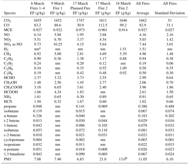
Table 2.Emission factors for the pine-dominated forest fires sampled in the mountains surrounding Mexico City in March 2006.
6 March 9 March 17 March 17 March 18 March All Fires All Fires Fires 1–4 Fire 1 Planned Fire Fire 2 Fire 2
Species EF (g/kg) EF (g/kg) EF (g/kg) EF (g/kg) EF (g/kg) Average Standard Deviation CO2 1655 1652 1747 1611 1646 1662 51
CO 83.2 88.6 30.9 112.5 99.2 82.9 31.1 MCE 0.927 0.922 0.973 0.901 0.914 0.927 0.027
NO 6.14 5.88 1.95 2.68 4.16 2.16
NO2 5.51 6.70 3.37 4.54 5.03 1.42
NOxas NO 9.73 10.25 4.15 5.64 7.44 3.01
H2 nma nm nm nm 1.51 1.51 nm
CH4 6.92 5.00 2.81 4.69 5.39 4.96 1.48
C2H4 0.90 0.36 1.38 1.17 0.88 0.94 0.38 C2H2 0.24 nm 0.20 0.12 nm 0.19 0.06
C2H6 0.34 nm 0.35 0.55 1.09 0.58 0.35 C3H6 0.19 nm 0.42 0.48 0.92 0.50 0.30
HCHO 2.37 3.32 3.73 2.55 2.99 0.64 CH3OH 1.48 2.56 1.45 2.77 2.06 0.70
CH3COOH 3.18 6.65 3.61 2.40 3.96 1.86
HCOOH 1.66 4.34 1.83 nm 2.61 1.50
NH3 1.81 0.65 0.30 0.89 0.91 0.65
HCN 1.50 0.32 1.67 0.60 1.02 0.66
propane 0.948 nm 0.141 0.069 0.386 0.488 isobutane 0.119 nm 0.015 nm 0.067 0.074 n-butane 0.326 nm 0.040 nm 0.183 0.202 t-2 butene 0.013 nm 0.030 0.044 0.029 0.016 1-butene 0.042 nm 0.086 0.105 0.078 0.032 isobutene 0.053 nm 0.072 0.118 0.081 0.033 c-2-butene 0.010 nm 0.021 0.031 0.021 0.011 cyclopentane 0.004 nm 0.002 nm 0.003 0.001 isopentane 0.032 nm 0.011 nm 0.022 0.015 n-pentane 0.051 nm 0.018 0.008 0.026 0.023 1,3 butadiene 0.042 nm 0.090 0.069 0.067 0.024 PM1 7.08 7.40 6.83 21.0 13.0b 11.05 6.10
anm indicates “not measured”
bThe 18 March particle measurement was of PM 2.5.
2.2.2 Estimation of fire-average, initial emission factors (EF)
We estimated fire-average, initial EF (g/kg) for PM1 and each observed trace gas from our fire-average, initial ERs using the carbon mass balance method (Yokelson et al., 1999). In brief, we assume that all the volatilized carbon is detected and that the fuel carbon content is known. By ignoring un-measured gases, we may inflate the emission factors by 1-2% (Andreae and Merlet, 2001). We assumed that all the fires burned in fuels containing 50% carbon by mass (Susott et al., 1996), but the actual fuel carbon percentage may vary by
±10% (2σ) of our nominal value. (EF scale linearly with as-sumed fuel carbon percentage.) The fire-average, initial EF for each compound and fire are listed in Table 2. Because NO is quickly converted to NO2after emission, we also report a
single EF for “NOxas NO.”
2.2.3 Determination of particle mass
The nephelometer was used to profile PM2.5per unit volume
of air (µg/m3)during plume penetrations of the 18 March fire. The LiCor simultaneously measured the mass of CO2
per unit volume of air during each pass through the plume. The ER (on a mass basis) for PM2.5to CO2for each fire (or
group of similar fires) was obtained by linear regression as above, except that the integrated excess mass values for each profile through the plume were used in lieu of grab sample excess mixing ratios. Assuming the particles were 60% car-bon by mass (Ferek et al., 1998) gave the contribution of PM2.5to the total carbon emitted for the emission factor
cal-culations. The PM2.5/CO2 mass ratio times EFCO2 (g/kg)
gave EFPM2.5(g/kg). The EFPM2.5for 18 March is likely
Because, the nephelometer was not available before 18 March, the UHSAS particle size data which was collected at a sample rate similar to that of the nephelometer (and from a nearby inlet that was also used for fast CO2measurements)
was used to determine particle mass as described next. We assumed spherical particles and integrated over the size distribution measured by the UHSAS, to obtain an es-timate of the volume of particles at 1 Hz. For each of the 8 plume penetrations on 18 March that featured both the UH-SAS and nephelometer sampling pine-forest fires in the MC-area mountains, the integrated particle mass was ratioed to the integrated particle volume. For the densest plumes, only data from the more dilute parts of the plume (<100µg/m3)
were used to avoid effects of saturation in the UHSAS. The mass to volume ratio was 1.858±0.183 g/cc. It is tempting to interpret this mass/volume ratio as an estimate of particle density, but the real density should be lower since: the par-ticles are not perfectly spherical, there is a small amount of particle mass in the diameter range 1–2.5 microns, and the particles are also∼8% black carbon by mass (Ferek et al., 1998; Reid et al., 2005), which would partially absorb the UHSAS laser. In any case, we used the above “empirical” m/v ratio to convert the integrated UHSAS particle volume to integrated particle mass for the pine forest fire, plume-penetration samples obtained 6–17 March. The simultane-ous co-located CO2measurements again provided the
com-parable integrated mass of CO2for each plume penetration.
The ER (on a mass basis) for PM1 to CO2 were used as
described above for the emission factor calculations. The EFPM1 values obtained as described above, may only be ac-curate to±25%, but are not large enough to introduce signifi-cant error in the trace gas EF. Because of the size distribution mentioned above, EFPM1 should be essentially equivalent to EFPM2.5
3 Results and discussion
3.1 Description and relevance of fires sampled
Detailed information about the MODIS and AVHRR hotspots detected in the entire country of Mexico since 2003 is conveniently tabulated at (http://www.conabio.gob.mx/ conocimiento/puntos calor/doctos/puntos calor.html). The data shows that fire activity increases gradually and then sharply from November to May before dropping to low levels by August. The months of March, April, and May accounted for about 12, 31, and 43% of the total MODIS hotspots from 2003–2006, respectively. Nationwide, March 2006 showed average activity for March not counting the 2003 El Nino year. However, Mexican Forestry personnel (personal communication to E. Alvarado) and casual inspection of MODIS hotspot maps produced by the University of Mary-land (UMD) Web Fire Mapper (http://maps.geog.umd.edu) (Justice et al., 2002) indicate that the level of fire activity in
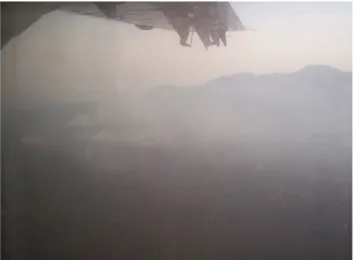
Fig. 2.Photo taken a few km northwest of the site of fire 3 6-F4 on 6 March at 5:13 p.m. local time. A large number of pine-forest fires are burning in, and mixing with, the MC outflow on a mountain pass to the south of the city.
March 2006 in the mountains around MC was above normal for March in that area and similar to levels that normally oc-cur in that area in April.
Table 1 shows location, time, and any fuel consumption and burned area information we have for the pine-forest fires that we were able to sample in the study area. Figure 1 shows all the MODIS UMD hotspots detected during March 2006 from 98–100 W and 19–20 N – the geographic limits of our MC-area study. Fire detections were made in the study area on 19 of the 31 days in March and totaled 218. The true number of fires is much larger as discussed below. Clouds or lack of coverage likely impacted the hotspot count on at least 14 of 31 days and that combined with a possible lack of sufficiently large fires at overpass time likely explain the days without detections. None of the fires that we sampled from the air in the study area registered as UMD-MODIS hotspots, because they were mostly short-lived (∼1 h) and occurred
>1 h before or after the Terra or Aqua overpass. However our fires were located in the precise areas showing the most hotspot activity. Thus, we conclude that (1) the number of hotspots provides a lower limit on the number of fires, (2) the hotspots are concentrated in the areas with the most burning, and (3) the fires we sampled were in the areas with the most burning.
y = -153.77x + 153.66
R2 = 0.4737
0 5 10 15 20 25
0.89 0.9 0.91 0.92 0.93 0.94 0.95 0.96 0.97 0.98
MCE
EFPM1
Fig. 3. Fire-average emission factors (EF) plotted versus fire-average modified combustion efficiency (MCE) for PM1 (data from Table 2). A range of EF occurs, which correlates with the relative amount of flaming and smoldering.
3.2 Initial emissions from pine-forest fires in MC-area mountains
Table 2 gives the EF for every species we detected for each fire (or group of similar fires) and the average and standard deviation for all the species measured. The standard devia-tion is a fairly large percentage of the average value for many species. Figure 3 shows EFPM1 vs MCE (index of the rel-ative amount of flaming and smoldering). Figure 3 suggests that much of the variability in EFPM1 is correlated with the different relative amounts of flaming and smoldering that oc-cur naturally on biomass fires. For nitrogen species there is also a contribution to variability from the differing fuel ni-trogen content (Yokelson et al., 1996, 2003a). The sum of the EF for VOC in Table 2 is 18.85 g/kg. However, oxy-genated VOC (OVOC) normally dominate the NMOC emit-ted by biomass fires and, in this study, we did not have the ca-pability to detect several OVOC common in biomass smoke (Christian et al., 2003). Therefore, we use 20 g/kg as a con-servative estimate of the real sum of VOC, which may be as high as 25 g/kg.
3.3 Comparison to other biomass burning emission factors and the influence of urban pollution on fire emissions
Most of the average EF shown in Table 2 are similar to pre-viously measured average values for forest burning. For in-stance, our study average EFPM1 (11±6 g/kg) agrees well with the recommended EFPM2.5 for extratropical forest
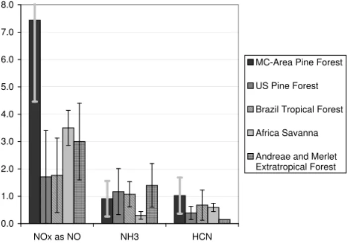
burning (13±7 g/kg) in Andreae and Merlet (2001). How-ever, large differences with previous forest fire measurements occur for NOxand HCN. In Fig. 4 we compare our EF for
NOx, HCN, and NH3, to those from other types of biomass
burning. In Fig. 4 the data for MC-area pine forest is from the present study. The data for US pine forest is an average from several published sources (Yokelson et al., 1996; Goode et al., 1999; Radke et al., 1991) and also includes some very similar unpublished lab-fire values obtained during the
fol-0.0 1.0 2.0 3.0 4.0 5.0 6.0 7.0 8.0
NOx as NO NH3 HCN
MC-Area Pine Forest
US Pine Forest
Brazil Tropical Forest
Africa Savanna
Andreae and Merlet Extratropical Forest
Fig. 4. Comparison of EF for selected nitrogen containing species between the MC-Area pine forest (affected by deposition), US Pine forest (in pristine area), tropical forest in Brazil, and savanna in Africa.
lowing studies (Christian et al., 20031). The Brazil tropical forest values are from a 2004 field campaign in the Ama-zon (Yokelson et al., 2007) and the African savanna data are from Yokelson et al. (2003a). The EF for extratropical for-est from the widely-used recommendations of Andreae and Merlet (2001) are also shown.
For NH3 the MC-area pine-dominated forest EF is close
to what has been measured for other forest burning and the recommendation of Andrea and Merlet. However for NOx
the MC-area pine forest EF is about 4 times typical measure-ments for other forests and more than twice the recommen-dation of Andrea and Merlet. For HCN the MC-area pine forest fire EF is about 3 times that measured for US pine forests and about twice that for tropical forests and savannas. Our EFHCN is almost 7 times higher than the recommen-dation of Andreae and Merlet. Our higher values for HCN could also indicate that a larger EF for acetonitrile (CH3CN)
is appropriate, but we did not measure the latter.
It is interesting that our average EF for NOx and HCN
are 3–4 times the average measured for US pine forests. The difference in the mean is statistically significant for NOx (7.44±3.0 MC-area, 1.71±1.7 US), whereas for HCN
the variability in the MC-area EF overlaps the US mean (1.023±0.66 MC-area, 0.39±0.24 US). Nevertheless, the in-dication is that the true HCN mean is also higher for the MC-area. We note that the MC-area forests are heavily impacted by deposition of MC pollutants (Fenn et al., 1999), whereas the US pine forest data is from pristine pine forest ecosys-tems. Thus we speculate that the high NOxand HCN
emis-sions in the MC-area pine forests may be due to enrichment
1Christian, T. J., Karl, T. G., Yokelson, R. J., Guenther, A., and
Fig. 5. Bright-field TEM image and EDS spectra of particles collected approximately 40 km south of the center of MC (sample 3 17-PF in Table 1 and Fig. 1a; collected 17 March 2006; start time 11:57:50, stop time 11:58:30 – local time,). They are the products of biomass burning (forest fire).(a)Image of various kinds of particles on a substrate of lacey carbon. OM – organic material, OM+K – organic material with inclusions of K compounds, S – sulfate, and S+K – ammonium and K sulfate.(b)EDS spectra for the particles in (a). The particle types were identified by their compositions and morphological properties. Numbers (1) to (6) in the inserts in (b) to (d) correspond to particles in the TEM image (a). The Cu peaks in the spectra are from the TEM grids.
of fuel nitrogen components that contribute to the emissions of these species via deposition of nitrogen-containing pollu-tants to the vegetation. The near-normal NH3emissions may
indicate that they arise from other more ubiquitous fuel nitro-gen components. These assumptions could be further tested in the future after we analyze the IR spectra from the pine forest fires sampled in less-polluted Mexican environments.
The observations of larger-than-normal NOx and HCN
emissions from the MC-area fires may also be relevant to understanding the local-regional atmospheric chemistry in other fire-impacted urban areas such as the Los Angeles basin where Radke et al. (1991) observed fire-induced resus-pension of CFC-12. In addition, Hegg et al. (1987) mea-sured higher emissions of NOx, SO2, and particle nitrate
from burning chaparral near Los Angeles than in the Pacific Northwest. In the latter study, the fuel types were differ-ent and the higher emissions of flaming compounds from chaparral were very likely partly due to the higher MCE of the chaparral fires, but deposition/resuspension probably also contributed to the difference as they suggested. In our study, we seem to support their hypothesis in a comparison of more similar fuel types. If industrial deposition does impact fire emissions, this could also be important in the southeastern US where widespread prescribed burning occurs near urban areas and in most urban areas in “developing countries” since they usually coexist with biomass burning.
3.4 Overview of particle chemistry
TEM studies show that many of the aerosol particles con-sist of internally mixed aggregates of several distinct particle types. For example, Fig. 5 shows a range of such particles (<0.3µm aerodynamic diameter) together with their compo-sitions, measured using energy dispersive X-ray spectrome-try (EDS). This sample was collected when the Twin Otter passed through the plume of the planned fire on 17 March. Identified particle types include soot, clay (probably kaolin-ite), tar balls, other organic material (OM), and a variety of sulfates and nitrates with and without K. The ammonium sul-fates as well as KNO3and, to a lesser extent, K2SO4tend to
NOx(see Sect. 3.3), the gaseous nitrogen may also contribute
to the N in OM particles and, conversely, particles may host an appreciable fraction of the emitted N.
3.5 Preliminary assessment of the contribution of fires to the MC-area plume
Fire emission factors (g/kg) can be multiplied by fuel con-sumption data (kg) to estimate total emissions at various scales. However, it is difficult to measure the amount of fuel burned for a large fire-prone geographic area. Consid-eration of the fires we sampled, combined with the MODIS hotspots, allows a crude estimate of the total fuel burned by mountain fires in the study area during March 2006. We base our rough estimate on the assumption that the planned fire had a size (22.2 ha), duration (∼1 h) and fuel consump-tion (6.54 Mg/ha) that is approximately average for the study area mountain fires. These assumptions seem conservative since the total fuel consumption of 145 Mg was about one-half the average total fuel consumption of 295 Mg for the 5 fires sampled by the ground crew in the area. We approx-imate the time period during which “average fires” burn as noon to five p.m. local time. (We choose noon as the be-ginning of the burning period because during one flight to southern Mexico we actually observed numerous fires being simultaneously ignited over a large, previously-clean area a few minutes after noon.) We note that cloud-free MODIS coverage of the study area (98–100 W and 19–20 N) during this “burning period” occurred on 2 of the 4 days (or one-half of the days) that the Twin Otter sampled fires there. If the average fire lasts for one hour, then an overpass during the burning period could detect up to one-fifth of the average fires if they were evenly distributed throughout the burning period. Coupling the above factors suggests that the actual number of mountain fires could be about 10 times larger than the 218 detected from space. Thus, 2180 fires times the total fuel consumption for the planned fire (145 Mg) estimates the total fuel consumption by these fires for the study area for March 2006, which is∼317 000 000 kg.
If the average fire duration is actually longer than the 1 h duration of the planned fire or if the number of fires peaks sharply at overpass time, then we have overestimated the number of fires, but this error could tend to be cancelled by the larger total fuel consumption expected for longer-lasting or more intense (mid-afternoon) fires. (The key assumption is the fuel consumption rate.) The study-area fuel consump-tion estimated this way may well be a lower limit since it does not account for fires that are obscured by the canopy, too small to register as hot spots (but potentially numerous), or large multi-day fires that would consume fuel for more than 5 h per day (several were observed from the Twin Ot-ter in restricted airspace and one was measured at∼300 ha by the ground crew). A good, satellite-based, burned area measurement for this region would reduce the uncertainties associated with our assumptions above, but is not available to
our knowledge. This estimate also explicitly leaves out any small-scale urban burning for cooking, garbage disposal etc. In any case, our estimated March 2006 study-area fuel consumption (317 000 000 kg) can be multiplied by any EF (g compound emitted per kg fuel burned) in Table 2 to estimate the total study-area emissions of that compound for the month produced by the mountain, pine-forest fires (hereinafter “mountain fires”). Our March 2006 mountain-fire CO emissions can be compared to 1/12 of the annual CO in the 2004 MC metropolitan area emissions inven-tory (MCMAEI, http://www.sma.df.gob.mx/sma/index.php? opcion=26{\&}id=392) and they represent about 18% of that value. Thus this analysis implies that these fires were respon-sible for about 15% of the CO exported in the March 2006 MC-area plume, although West et al. (2004) argued that the CO and VOC emissions may be underestimated in the MC-MAEI. Our preliminary, bottom-up estimate suggests simi-lar fire contributions to the total for NOx(14%), NH3(16%),
and VOC (12%) and coincidentally the upper limit for the NOx/VOC mass ratio from fires (∼0.38) is similar to that in
the MCMAEI (∼0.34). In contrast to the similar tions calculated for the trace gases above, the fire contribu-tion to the primary PM10 is estimated to be much larger at
67%. The true contribution could be higher since PM1/PM10
from fires is about 0.7 (Andreae and Merlet, 2001). Com-paring to the MCMAEI PM2.5suggests that 86% of the
pri-mary PM2.5produced in the study area is from the mountain
fires. The above estimates also do not include the fire emis-sions due to any other biomass burning not sampled by our aircraft (Bertschi et al., 2003a; Yevich and Logan, 2003). Another relevant insight is derived by noting that the pri-mary PM10/CO and PM2.5/CO mass ratios in the MCMAEI
are∼0.0115 and 0.0037, respectively; whereas the primary PM1/CO ratio from mountain fires was∼0.133. Thus, re-gardless of the fire fraction of CO in the MC-area plume, the fire fraction of primary fine PM should be much greater.
The contribution of fire emissions to the MC-area plume can be estimated by another approach since HCN and CH3CN are both thought to be emitted primarily by biomass
the days of the downwind measurements, (2) that other types of biomass burning in the study area may be ignored, and (3) that our airborne measurements of the fire ER HCN/CO are also valid for any initially-unlofted smoldering fire emissions (Bertschi et al., 2003b). The third assumption is supported by the fact that EFHCN are not strongly dependent on MCE in this work (or in Africa (Yokelson et al., 2003a) or Brazil (Yokelson et al., 2007)).
Explicitly, the average MC-area mountain-fire molar ER for HCN/CO measured during MILAGRO is 0.012±0.007 (combining 0.0128±0.0096 from the Twin Otter and 0.011 from the single MC-area fire measurement of HCN/CO on the C-130, which is in good agreement with the Twin Otter mean). The average outflow HCN/CO molar ratio measured on the C-130 was about 0.003±0.0003 implying that about 25% of the study area CO was from the mountain fires we sampled. This is actually fairly consistent with our crude bottom-up estimate above. Note, that use of fire HCN/CO ER from the other sources shown in Fig. 4 would have increased the estimate of the biomass burning contribution by a factor of 2–9. Given the large uncertainty in both the urban and fire emissions mentioned above, it would be useful to develop estimates based on additional biomass burning indicators if possible (e.g. CH3CN, CH3Cl, particle14C, etc.).
We can go a step further with the “tracer-based analysis” since according to the fire and urban primary PM/CO ra-tios quoted above; a 25% fire contribution to study-area CO implies fire contributions to study-area primary PM10 and
PM2.5of 79% and 92%, respectively. We again emphasize
that these fractional values depend strongly on the accuracy of our fuel consumption estimate and the MCMAEI (e.g. if the MCMAEI primary PM2.5was higher, then our estimate
of the fire fraction of primary PM2.5produced in the study
area would be lower). However, it is interesting that this sec-ond, partially-independent approach also suggests that fires are the main source of primary, fine-particle mass in our study area in March 2006. Finally we note that in both the bottom-up estimate and the HCN-based analysis we have so far ignored how other types of biomass burning in the study area (e.g. cooking, garbage burning, etc.) would affect an es-timate of the fire contribution to the MC-area outflow. In the case of the bottom up estimate, adding more types of burn-ing increases the overall fire contribution. We can also de-duce the likely affect on the tracer-based estimates as fol-lows. Bertschi et al. (2003a) found that HCN was below their detection limits for cooking fires. Thus, most likely, the HCN/CO ratio for the other types of burning is lower than for the mountain fires and the same HCN/CO ratio in the outflow would then imply that biomass burning as a whole makes a larger contribution to the outflow CO and particulate.
In addition to the near-source mixing of fire and urban emissions in the MC-area plume, we note that the more aged MC-area plume also likely interacts with biomass burning emissions from other regions of Mexico. For example, on 12 March and 29 March the Twin Otter sampled (mostly)
widespread agricultural waste burning (also characterized by relatively high N emissions) on the western Yucatan penin-sula. On both of these days, HYSPLIT forward trajectories from the western Yucatan fires trend to the NW and pass close to the NE-trending forward trajectories from MCMA over the Gulf of Mexico (Draxler and Rolph, 2003). The projected mixing would be after emissions from both sources had aged 1–3 days. To aid in modeling this potential inter-action, the Twin Otter sampled approximately 20 fires on the Yucatan and the C-130 also sampled 3 fires there. The results for those fires will be presented in a separate paper.
Even if the MC plume does not mix with additional down-wind fire or urban emissions, the particles observed hours to days downwind from MC will reflect both the primary emis-sions from our study area and secondary processes such as oxidation, coagulation, and secondary organic and inorganic aerosol formation. Secondary processes make a strict source apportionment less rigorous. For instance gases from fos-sil fuel sources can condense on biomass burning particles and vice versa. Biogenic emissions can condense on both types of particles. A biomass burning particle can coagulate with a particle generated from fossil fuel combustion mak-ing a larger particle with an ambiguous source. Particle con-stituents could evaporate and then recondense (with or with-out oxidation) onto other particles (Robinson et al., 2007). A full analysis of these issues would require a modeling study similar to that of Olcese et al. (2007).
However, it is of interest to consider secondary processes (ignoring mixing of the two particle sources considered in this paper) and then roughly re-estimate the mass contri-bution of the two sources to the downwind plume. The secondary process with the most potential to alter source PM/CO ratios is secondary aerosol formation. Secondary aerosol formation is promoted by the presence of large amounts of condensable gases or high levels of O3, which
can convert volatile NMOC to condensable gases (Reid et al., 1998; Olcese et al., 2007; Kang et al., 2007). Both of these factors are present in abundance for both sources in our study area.
The mass ratio for primary particles to CO in the MCMA EI is 0.0115. According to DeCarlo (attributed comment2) and references therein (e.g. Salcedo et al., 2006) a mass ra-tio for PM/CO that realistically includes secondary aerosol formation in the fossil-fuel aerosol from the MC area would range from 0.04 to 0.08. This represents an increase over the MCMA EI PM10 by a factor of 3.5–7. PM/CO is also
likely to increase in the biomass burning aerosol. Moffet et al. (2007) measured a factor of 1.6 increase in the volume of biomass burning particles aged for several hours in the MC-urban area during MILAGRO. A review article on biomass
2DeCarlo, P.: Interactive comment on “Emissions from forest
burning particles by Reid et al. (2005) gives many examples of biomass burning aerosol mass (ratioed to CO) increasing by factors from 1.7 to 2.0 over 1–3 days in the absence of significant contributions from other sources (see also Reid et al., 1998). Growth factors as low as 1.2 have not been mea-sured for biomass burning aerosol, but we adopt that factor as our lower limit for fires. This is justified by using the 2004 MCMAEI and our Table 2 and then assuming that the same percentage of co-emitted gas-phase precursors condense onto the biomass burning particles as is implied by our lower limit of 0.04 PM/CO for the urban aerosol. This could be reason-able because it essentially assumes that similar chemistry and physics affect the two types of combustion particles. We do not consider evaporation of gases from the particles for ei-ther source because strong evidence exists that on real fires significant growth in PM accompanies large∼50-fold dilu-tion of the emissions (Ward et al., 1992; Babbitt et al., 1996). The range of growth factors we consider for biomass burn-ing aerosol is much smaller than that for fossil fuel aerosol, but corresponds to the addition of similar mass. In fact, more mass could add to the biomass burning particles since the fire particles are produced at higher elevation, which implies that more O3and UV and lower temperatures (favoring
conden-sation) are relevant. In addition, the forest fire particles are produced in an environment likely to have higher concentra-tions of biogenic emissions and the NMOC gases co-emitted by fires are much more reactive than for fossil fuel combus-tion (Reid et al., 1998; Christian et al., 2004).
We now re-estimate a range of mass fractions in the MC-area outflow under the approximation of just two sources (mountain pine forest fires and MCMA). A lower estimate for the fire, fine-particle mass contribution in the outflow is 40% (60% from MCMA). This is obtained by starting with our HCN-based estimate of the fire contribution to study-area CO and then assuming that the PM/CO mass ratio in the aged MCMA aerosol should be 0.08 and that our fire PM/CO should be multiplied by 1.2 to account for secondary aerosol formation. A higher fire contribution is estimated by assuming a mass-growth factor of 2 for biomass burning and a PM/CO mass ratio of 0.04 for the MCMA aerosol. In this case the fire contribution is estimated as 69% (31% MCMA contribution). The midpoint of this range corresponds to 55% of the fine particle mass in the MC-area outflow being due to the mountain fires. Of course, different assumptions, addi-tional downwind data, or a detailed modeling exercise could lead to adjustments in these estimates.
3.6 Possible nature of fire impacts on the MC-area plume photochemistry
The main purpose of this paper is to present the study area EF and a preliminary assessment of their significance. Hav-ing established that fires will likely produce a visible sig-nal in the MC-area plume measurements we now list some fairly obvious potential influences of fires on the plume
pho-tochemistry. Introductory material about these affects can be found in atmospheric chemistry textbooks (Finlayson-Pitts and Pitts, 1986). For example, the injection of fresh “fire-NOx” into the MC plume immediately downwind of MC
could contribute to the measured change in the NOx/NOy
ratio between downtown MC and further downwind. Both NOxand VOC from fires could alter the downwind O3
pro-duction (which could also be impacted by the high dust lev-els observed (Moffet et al., 2007)). NOx from fires could
also contribute to aerosol nitrate (Fig. 5). Ammonia is an-other reactive fire emission that could contribute to aerosol particles such as ammonium sulfate or ammonium bisulfate and affect secondary aerosol formation in general. The parti-cles emitted by fires are enriched in organic carbon (Fig. 5a) compared to particles from industrial sources and this could affect observed downwind heterogeneous chemistry. Also, the addition of organic rich particles to the MC plume by fires should not be confused with secondary aerosol forma-tion. Confirmation of any of these impacts may be found in the MILAGRO airborne data.
3.7 Relevance to ground-based measurements in the Mex-ico City basin
Previous atmospheric chemistry measurements in the MC-area were nearly all ground-level measurements in the heart of the MC urban area. An influence of biomass burning was recognized in some of these reports. Bravo et al. (2002) an-alyzed the particulate data for the MC urban area from 1992 to 1999. They observed some large increases in urban PM10
and total suspended particulate (TSP) during March-May of 1998, which they attributed to greatly increased biomass burning in Mexico at that time (Galindo et al., 2003). Moya et al. (2003) analyzed urban MC particulate from December 2000 to October 2001. There was a marked peak in total loading during April of 2001, which coincides with the usual annual peak of fire activity in the area.
not be expected to find their way to downtown MC. Even for directly upwind mountain fires, much of the emissions could pass above ground-level monitors.
As part of the March 2006 MILAGRO campaign, at least two ground-based studies focused on source apportionment for particles, in the MC basin, during roughly the same time period as our airborne measurements. Stone et al. (2007) estimated that biomass burning accounted for 5–50% of the organic carbon in particles collected on filters in the Mexico City basin. At a downtown MC site during MILAGRO, Mof-fet et al. (2007) found that particles with a biomass-burning core accounted for the largest number fraction (41%) of sub-micron, ambient particles. The results of both of these stud-ies would have been partially affected by types of biomass burning other than the mountain fires that we directly sam-pled from the air and discuss in this paper. Nevertheless, as explained above, both of these estimates are consistent with our preliminary source apportionment for the outflow.
4 Conclusions
The MILAGRO experiment was conducted to further the understanding of the outflow from the Mexico City (MC) area. This paper presents data that is useful for modeling the biomass burning contribution to the outflow photochem-istry that arises due to fires in the pine-dominated forests lo-cated in the mountains around MC. The average forest fire emissions of HCN were∼2 times higher than normally ob-served for forest fires, which should be taken into account in source apportionment. The average forest fire emissions of NOx were 2–4 times higher than would be assumed based
on literature values. This is important in modeling plume photochemistry. The high N emissions from MC-area forest fires may be relevant to understanding atmospheric chemistry throughout the world in the many urban areas that coexist with biomass burning.
For source apportionment purposes, we designate the re-gion from 19–20◦N and 98–100◦W (which includes MC and the adjacent mountains) as the “Mexico City area.” Prelim-inary “bottom-up” or “tracer-based” analysis then suggests that mountain fires produced about 15 or 25%, respectively, of the CO, and similar percentages of VOC, NH3, and NOx
in the MC area in March 2006; but a much larger percentage (67–92%) of the primary fine particles. Assuming the moun-tain fire contribution to the CO in the March 2006 MC-area outflow is 25% (based on the HCN/CO ratios) and coupling with a range of values for secondary aerosol formation in the urban and forest fire emissions suggests that about 40– 69% (55% midpoint) of the fine particle mass in the outflow was from the mountain fires. Coupling the uncertainty in the HCN/CO ratios with the above analysis suggests that the March 2006 mountain fire contribution to the MC-area out-flow fine particle mass was approximately 50±30% (i.e. 20– 80%). The large range highlights the need for more work.
However, it is interesting that our “bottom-up” and “tracer-based” approaches to these estimates agreed well. Taken together they suggest that biomass burning is a significant component of the MC-area outflow during the biomass burn-ing season in Mexico (March–May). There are likely days of higher and lower fire influence on the outflow, but fires are probably a significant influence, on average, during these three months. Further, we do not claim that Mexico City’s air quality problems could be solved by eliminating regional biomass burning, but there is a strong possibility that the application of smoke management techniques (Hardy et al., 2001) to regional biomass burning could improve the March– May Mexico City air quality.
Acknowledgements. The authors thank Eric Hintsa and NSF for
emergency supplemental funding that made it possible for ASU, U Miami, and U Colorado to conduct measurements on the Twin Otter. We thank the Twin Otter pilots E. Thompson, G. Moore, J. Stright, A. Knobloch, and mechanic K. Bailey. Special thanks go to S. Madronich, L. Molina, and J. Meitin for their dedication to making the MILAGRO campaign a success for all. The University of Montana, the planned fire, and the airborne research was supported largely by NSF grant ATM-0513055. Yokelson was also supported by the Rocky Mountain Research Station, Forest Service, U.S. Department of Agriculture (agreement 03-UV-11222049-046). The USFS science team and partial support for the airborne research was provided by the NASA North American Carbon Plan (NNHO5AA86I). Participation by Arizona State University was supported by NSF grant ATM-0531926. Electron Microscopy was performed at the John M. Cowley Center for High Resolution Microscopy at Arizona State University. Support to the University of Miami was provided by NSF (ATM 0511820). X. Zhu and L. Pope provided excellent technical support for the canister trace gas analyses. Support for operation of the Caltech CIMS instrument was provided by NASA (NNG04GA59G) and by EPA-STAR support for J. Crounse. We also thank the fire staff of Mexico’s Comision Nacional Forestal in the states of Morelos, Mexico, Distrito Federal, and the Guadalajara Head-quarters for the execution of the prescribed fire in the state of Morelos and for logistical support to conduct post-fire assess-ment of several fires of opportunity flown by the Twin Otter aircraft.
Edited by: L. Molina
References
Andreae, M. O. and Merlet, P.: Emission of trace gases and aerosols from biomass burning, Global Biogeochem. Cy., 15(4), 955–966, doi:10.1029/2000GB001382, 2001.
Arai, M.: Continuous analysis of vehicle exhaust gas by Fourier transform infrared spectroscopy, Anal. Sci., 9, 77–82, 1993. Babbitt, R. E., Ward, D. E., Susott, R. A., Artaxo, P., and Kaufmann,
J. B.: A comparison of concurrent airborne and ground based emissions generated from biomass burning in the Amazon Basin, SCAR-B Proceedings, Transtec, Sa˜o Paulo, Brazil, 1996. Bertschi, I. T., Yokelson, R. J., Ward, D. E., Christian, T .J., and
transform infrared spectroscopy, J. Geophys. Res., 108(D13), 8469, doi:1029/2002/D002158, 2003a.
Bertschi, I. T., Yokelson, R. J., Ward, D. E., Babbitt, R. E., Susott, R. A., Goode, J. G., and Hao, W. M.: Trace gas and particle emissions from fires in large-diameter and be-lowground biomass fuels, J. Geophys. Res., 108(D13), 8472, doi:10.1029/2002JD002100, 2003b.
Bravo, A. H., Sosa, E. R., Sanchez, A. P., Jaimes, P. M., and Saave-dra, R. M. I.: Impact of wildfires on the air quality of Mexico City, 1992–1999, Environ. Poll., 117, 243–253, 2002.
Brown, I. F., Schroeder, W., Setzer, A., de Los Rios Maldonado, M., Pantoja, N., Duarte, A., and Marengo, J.: Monitoring fires in southwestern Amazonia rain forests, EOS Trans. AGU, 87(26), 253–264, 2006.
Brown, J. K.: Handbook for inventorying down woody material, General Technical Report INT-16, Ogden UT, U.S. Department of Agriculture, Forest Service Intermountain Research Forest and Range Experiment Station, 23 pp., 1974.
Christian, T., Kleiss, B., Yokelson, R. J., Holzinger, R., Crutzen, P. J., Hao, W. M., Saharjo, B. H., and Ward, D. E.: Comprehen-sive laboratory measurements of biomass-burning emissions: 1. Emissions from Indonesian, African, and other fuels, J. Geophys. Res., 108(D23), 4719, doi:10.1029/2003JD003704, 2003. Comisi´on Nacional para el Conocimiento y Uso de la
Biodi-versidad (CONABIO): Uso de suelo y vegetaci´on modificado por CONABIO, Escala 1:1 000 000, Comisi´on Nacional para el Conocimiento y Uso de la Biodiversidad, Mexico City, Mexico, 1999.
Crounse, J. D., McKinney, K. A., Kwan, A. J., and Wennberg, P. O.: Measurement of gas-phase hydroperoxides by chemical ioniza-tion mass spectrometry, Anal. Chem., 78(19), 6726–6732, 2006. de Gouw, J. A., Warneke, C., Stohl, A., et al.: Volatile organic com-pounds composition of merged and aged forest fire plumes from Alaska and western Canada, J. Geophys. Res., 111, D10303, doi:10.1029/2005JD006175, 2006.
Draxler, R. R. and Rolph, G. D.: HYSPLIT (HYbrid Single-Particle Lagrangian Integrated Trajectory) Model access via NOAA ARL READY Website (http://www.arl.noaa.gov/ready/hysplit4.html), NOAA Air Resources Laboratory, Silver Spring, MD, 2003. Fast, J. D., de Foy, B., Acevedo Rosas, F., et al.: A
meteorologi-cal overview of the MILAGRO field campaigns, Atmos. Chem. Phys., 7, 2233–2257, 2007,
http://www.atmos-chem-phys.net/7/2233/2007/.
Fenn, M. E., de Bauer, L. I., Quevedo-Nolasco, A., and Rodriquez-Frausto, C.: Nitrogen and sulfur deposition and forest nutrient status in the Valley of Mexico, Water Air Soil Poll., 113, 155– 174, 1999.
Ferek, R. J., Reid, J. S., Hobbs, P. V., Blake, D. R., and Liousse, C.: Emission factors of hydrocarbons, halocarbons, trace gases, and particles from biomass burning in Brazil, J. Geophys. Res., 103(D24), 32 107–32 118, doi:10.1029/98JD00692, 1998. Finlayson-Pitts, B. J. and Pitts Jr., J. N.: Atmospheric Chemistry:
Fundamentals and Experimental Techniques, John Wiley, Inc., New York, 1098 pp., 1986.
Flocke, F., Herman, R. L., Salawitch, R. J., et al.: An exami-nation of the chemistry and transport processes in the tropical lower stratosphere using observations of long-lived and short-lived compounds obtained during STRAT and POLARIS, J. Geo-phys. Res., 104, 26 625–26 642, 1999.
Galindo, I., Lopez-Perez, P., and Evangelista-Salazar, M.: Real-time AVHRR forest fire detection in Mexico (1998–2000), Int. J. Remote Sens., 24, 9–22, 2003.
Gerbig, C., Schmitgen, S., Kley, D., Volz-Thomas, A., Dewey, K., and Haaks, D.: An improved fast-response vacuum-UV reso-nance fluorescence CO instrument, J. Geophys. Res., 104, 1699– 1704, 1999.
Goode, J. G., Yokelson, R. J., Susott, R. A., and Ward, D. E.: Trace gas emissions from laboratory biomass fires measured by open-path FTIR: Fires in grass and surface fuels, J. Geophys. Res., 104(D17), 21 237–21 245, doi:10.1029/1999JD900360, 1999. Goode, J. G., Yokelson, R. J., Ward, D. E., Susott, R. A.,
Bab-bitt, R. E., Davies, M. A., and Hao, W. M.: Measurements of excess O3, CO2, CO, CH4, C2H4, C2H2, HCN, NO, NH3,
HCOOH, CH3COOH, HCHO, and CH3OH in 1997 Alaskan
biomass burning plumes by airborne Fourier transform infrared spectroscopy (AFTIR), J. Geophys. Res., 105(D17), 22 147– 22 166, doi:10.1029/2000JD900287, 2000.
Hand, J. L., Malm, W. C., Laskin, A., et al.: Optical, physical, and chemical properties of tar balls observed during the Yosemite Aerosol Characterization Study, J. Geophys. Res., 110, D21210, doi:10.1029/2004JD005728, 2005.
Hao, W. M., Ward, D. E., Olbu, G., and Baker, S. P.: Emissions of CO2, CO, and hydrocarbons from fires in diverse African
sa-vanna ecosystems, J. Geophys. Res., 101, 23 577–23 584, 1996. Hardy, C., Ottmar, R., Peterson, J., Core, J., Seamon, P. (Eds.):
Smoke Management Guide for Prescribed and Wildland Fire, 2001 Edition, National Interagency Fire Center, Boise, ID, US, 226 pp., 2001.
Hegg, D. A., Radke, L. F., Hobbs, P. V., and Brock, C. A.: Nitrogen and sulfur emissions from the burning of forest products near large urban areas, J. Geophys. Res., 92, 14 701–14 709, 1987. Hobbs, P.V., Sinha, P., Yokelson, R. J., Christian, T. J., Blake, D. R.,
Gao, S., Kirchstetter, T. W., Novakov, T., and Pilewskie, P.: Evo-lution of gases and particles from a savanna fire in South Africa, J. Geophys. Res., 108(D13), 8485, doi:10.1029/2002JD002352, 2003.
Instituto Nacional de Estad´ıstica, Geograf´ıa e Inform´atica (INEGI) and Instituto Nacional de Ecolog´ıa (INE): Uso de suelo y veg-etaci´on: Agrupado por CONABIO: Escala 1:1 000 000, Mexico City, Mexico, 1998.
Jonsson, H. H., Wilson, J. C., Brock, C. A., et al.: Performance of a focused cavity aerosol spectrometer for measurements in the stratosphere of particle size in the 0.06–2.0µm diameter range, J. Ocean. Atmos. Technol., 12, 115–129, 1995.
Johnson, K. S., de Foy, B., Zuberi, B., Molina, L. T., Molina, M. J., Xie, Y., Laskin, A., and Shutthanadan, V.: Aerosol composi-tion and source apporcomposi-tionment in the Mexico City metropolitan area with PIXE/PESA/STIM and multivariate analysis, Atmos. Chem. Phys. 6, 4591–4600, 2006.
Justice, C. O., Giglio, L., Korontzi, S., Owens, J., Morisette, J. T., Roy, D., Descloitres, J., Alleaume, S., Petitcolin, F., and Kauf-man, Y.: The MODIS fire products, Remote Sens. Environ., 83, 244–262, 2002.
Kang, E., Root, M. J., and Brune, W. H.: Introducing the concept of Potential Aerosol Mass (PAM), Atmos. Chem. Phys. Discuss., 7, 9925–9972, 2007,
aerosol particles from biomass burning in southern Africa: 2. Compositions and aging of inorganic particles, J. Geophys. Res., 108(D13), 8484, doi:10.1029/2002JD002310, 2003.
Li, Q., Jacob, D. J., Bey, I., Yantosca, R. M., Zhao, Y., Kondo, Y., and Notholt, J.: Atmospheric hydrogen cyanide (HCN): biomass burning source, ocean sink?, Geophys. Res. Lett., 27(3), 357– 360, doi:10.1029/1999GL010935, 2000.
Loveland, T. R., Reed, B. C., Brown, J. F., Ohlen, D. O., Zhu, J., Yang, L., and Merchant, J. W.: Development of a Global Land Cover Characteristics Database and IGBP DISCover from 1-km AVHRR Data, Int. J. Remote Sens., 21, 1303–1330, 2000. Moffet, R. C., de Foy, B., Molina, L. T., Molina, M. J., and Prather,
A.: Measurement of ambient aerosols in northern Mexico City by single particle mass spectrometry, Atmos. Chem. Phys. Discuss., 7, 6413–6457, 2007,
http://www.atmos-chem-phys-discuss.net/7/6413/2007/. Molina, L. T., Kolb, C. E., de Foy, B., Lamb, B. K., Brune, W. H.,
Jimenez, J. L., and Molina, M. J.: Air quality in North America’s most populous city – overview of MCMA-2003 campaign, At-mos. Chem. Phys., 7, 2447–2473, 2007,
http://www.atmos-chem-phys.net/7/2447/2007/.
Nance, J. D., Hobbs, P. V., Radke, L. F., and Ward, D. E.: Airborne measurements of gases and particles from an Alaskan wildfire, J. Geophys. Res., 98, 14 873–14 882, 1993.
Olcese, L. E., Penner, J. E., and Sillman, S.: Development of a sec-ondary organic aerosol formation mechanism: comparison with smog chamber experiments and atmospheric measurements, At-mos. Chem. Phys. Discuss., 7, 8361–8393, 2007,
http://www.atmos-chem-phys-discuss.net/7/8361/2007/. P´osfai, M., Simonics, R., Li, J., Hobbs, P. V., and Buseck,
P. R.: Individual aerosol particles from biomass burning in southern Africa: 1. Compositions and size distributions of carbonaceous particles, J. Geophys. Res., 108(D13), 8483, doi:10.1029/2002JD002291, 2003.
P´osfai, M., Gelencs´er, A., Simonics, R., Arat´o, K., Li, J., Hobbs, P. V., and Buseck, P. R.: Atmospheric tar balls: Particles from biomass and biofuel burning, J. Geophys. Res., 109, D06213, doi:10.1029/2003JD004169, 2004.
Radke, L.F., Hegg, D. A., Hobbs, P. V., Nance, J. D., Lyons, J. H., Laursen, K. K., Weiss, R. E., Riggan, P. J., and Ward, D. E.: Particulate and trace gas emissions from large biomass fires in North America, in: Global Biomass Burning: Atmospheric, Climatic, and Biospheric Implications, edited by: Levine, J. S., MIT Press, Cambridge, 209–224, 1991.
Reid, J. S., Hobbs, P. V., Ferek, R. J., Blake, D. R., Martins, J. V., Dunlap, M. R., and Liousse, C.: Physical, chemical, and opti-cal properties of regional haze dominated by smoke in Brazil, J. Geophys. Res., 103, 32 059–32 080, 1998.
Reid, J. S., Koppmann, R., Eck, T. F., and Eleuterio, D. P.: A review of biomass burning emissions part II: intensive physical proper-ties of biomass burning particles, Atmos. Chem. Phys., 5, 799– 825, 2005,
http://www.atmos-chem-phys.net/5/799/2005/.
Robinson, A. L., Donahue, N. M., Shrivastava, M. K., Weitkamp, E. A., Sage, A. M., Grieshop, A. P., Lane, T. E., Pierce, J. R., and Pandis, S. N.: Rethinking organic aerosols: Semivolatile emis-sions and photochemical aging, Science, 315(5816), 1259–1262, 2007.
Salcedo, D., Onasch, T. B., Dzepina, K., et al.: Characterization
of ambient aerosols in Mexico City during the MCMA-2003 campaign with Aerosol Mass Spectrometry: results from the CENICA Supersite, Atmos. Chem. Phys., 6, 925–946, 2006, http://www.atmos-chem-phys.net/6/925/2006/.
Shim, C., Wang, Y., Singh, H. B., Blake, D. R., and Guenther, A. B.: Source characteristics of oxygenated volatile organic com-pounds and hydrogen cyanide, J. Geophys. Res., 112, D10305, doi:10.1029/2006JD007543, 2007.
Stone, E. A., Snyder, D. C., Sheesley, R. J., Sullivan, A. P., Weber, R. J., and Schauer, J. J.: Source apportionment of fine organic aerosol in Mexico City during the MILAGRO Experiment 2006, Atmos. Chem. Phys. Discuss., 7, 9635–9661, 2007,
http://www.atmos-chem-phys-discuss.net/7/9635/2007/. Susott, R. A., Olbu, G. J., Baker, S. P., Ward, D. E., Kauffman,
J. B., and Shea, R.: Carbon, hydrogen, nitrogen, and thermo-gravimetric analysis of tropical ecosystem biomass, in: Biomass Burning and Global Change, edited by: Levine,J. S., MIT Press, Cambridge, 350–360, 1996.
Trent, A., Davies, M. A., Fisher, R., Thistle, H., and Babbitt, R.: Evaluation of optical instruments for real-time, continuous mon-itoring of smoke particulates, Tech. Rep. 0025 2860 MTDC, USDA Forest Service, Missoula Technology and Development Center, Missoula, Mont., 38 pp., 2000.
Ward, D. E. and Radke, L. F.: Emissions measurements from veg-etation fires: A comparative evaluation of methods and results, in: Fire in the Environment: The Ecological, Atmospheric and Climatic Importance of Vegetation Fires, edited by: Crutzen, P. J. and Goldammer, J. G., John Wiley, New York, 53–76, 1993. Ward, D. E., Susott, R. A., Waggoner, A. P., Hobbs, P. V., and
Nance, J. D.: Emission factor measurements for two fires in British Columbia compared with results for Oregon and Wash-ington, in: Proceedings of Pacific Northwest International Sec-tion of the Air and Waste management AssociaSec-tion Annual Meet-ing, Bellevue, WA, 11–13 November, 1992.
Weinheimer, A. J., Montzka, D. D., and Campos, T. L., et al.: Com-parison of DC-8 and ER-2 species measurements on 8 February 1996: NO, NOy, O3, CO2, CH4, and N2O, J. Geophys. Res.,
103, 22 087–22 096, 1998.
West, J., Zavala, M. A., Molina, L. T., Molina, M. J., Martini, F. S., McRae, G. J., Sosa-Iglesias, G., and Arriaga-Colina, J. L.: Mod-eling ozone photochemistry and evaluation of hydrocarbon emis-sions in the Mexico City metropolitan area, J. Geophys. Res., 109, D19312, doi:10.1029/2004JD004614, 2004.
Yokelson, R .J., Karl, T. G., Artaxo, P., Blake, D. R., Christian, T. J., Griffith, D. W. T., Guenther, A., and Hao, W. M.: The tropical forest and fire emissions experiment: Overview and airborne fire emission factor measurements, Atmos. Chem. Phys., 7, 5175– 5196, 2007,
http://www.atmos-chem-phys.net/7/5175/2007/.
Yokelson, R. J., Bertschi, I. T., Christian, T. J., Hobbs, P. V., Ward, D. E., and Hao, W. M.: Trace gas measurements in nascent, aged, and cloud-processed smoke from African savanna fires by air-borne Fourier transform infrared spectroscopy (AFTIR), J. Geo-phys. Res., 108(D13), 8478 doi:10.1029/2002JD002322, 2003a. Yokelson, R. J., Christian, T. J., Bertschi, I. T., and Hao, W. M.: Evaluation of adsorption effects on measurements of ammonia, acetic acid, and methanol, J. Geophys. Res., 108(D20), 4649 doi:10.1029/2003JD003549, 2003b.
R. E., Wade, D. D., Bertschi, I., Griffith, D. W. T., and Hao, W. M.: Emissions of formaldehyde, acetic acid, methanol, and other trace gases from biomass fires in North Carolina measured by air-borne Fourier transform infrared spectroscopy, J. Geophys. Res., 104(D23), 30 109–30 126, doi:10.1029/1999JD900817, 1999.