A COMPARATIVE ANALYSIS OF THREE METAHEURISTIC METHODS APPLIED TO FUZZY COGNITIVE MAPS LEARNING
Bruno A. Ang´elico
1*, M´arcio Mendonc¸a
1, Taufik Abr˜ao
2and L´ucia Val´eria R. de Arruda
3Received February 14, 2012 / Accepted June 22, 2013
ABSTRACT.This work analyses the performance of three different population-based metaheuristic ap-proaches applied to Fuzzy cognitive maps (FCM) learning in qualitative control of processes. Fuzzy cog-nitive maps permit to include the previous specialist knowledge in the control rule. Particularly, Particle Swarm Optimization (PSO), Genetic Algorithm (GA) and an Ant Colony Optimization (ACO) are con-sidered for obtaining appropriate weight matrices for learning the FCM. A statistical convergence analysis within 10000 simulations of each algorithm is presented. In order to validate the proposed approach, two industrial control process problems previously described in the literature are considered in this work. Keywords: Fuzzy Cognitive Maps, Particle Swarm Optimization, Genetic Algorithm, process control, statistical convergence analysis.
1 INTRODUCTION
Fuzzy Cognitive Maps are signed and directed graph, in which the involved variables are fuzzy numbers. They were initially proposed by Kosko [1, 2, 3], as an extension of cognitive maps proposed by Axelrod [4]. The graph nodes represent linguistic concepts modeled by fuzzy sets and they are linked with other concepts through fuzzy connections. Each of these connections has a numerical value (weight) taken from a fuzzy set, which models the relationship strength among concepts. In addition, FCM can be considered a type of cognitive neuro-fuzzy network, which is initially developed by the acquisition of expert knowledge, but can be trained by several supervised and/or unsupervised techniques as reviewed in [5].
There are in the literature several models based on fuzzy cognitive maps developed and adapted to a large range of applications, such as political decision [6], medical decision [7, 8], indus-trial process control [9, 10], artificial life [11], social systems [12], corporative decision, policy
*Corresponding author
1Federal University of Technology – Paran´a (UTFPR), Corn´elio Proc´opio, Brazil. E-mails: bangelico@utfpr.edu.br; mendonca@utfpr.edu.br
2State University of Londrina – Paran´a (UEL), Londrina, Brazil. E-mail: taufik@uel.br
analysis [13], among others. A good survey of recent applications is given by Papageorgiou e Salmeron in [14].
A FCM construction can be done in the following manner:
• Identification of concepts and its interconnections determining the nature (positive, nega-tive or null) of the causal relationships between concepts.
• Initial data acquisition by the expert opinions and/or by an equation analysis when the mathematical system model is known.
• Submitting data from expert opinions to a fuzzy system which output represents the FCM weights.
• Weight adaptation and optimization of the initially proposed FCM, adjusting its response to the desired output.
• Validation of the adjusted FCM.
However, when the experts are not able to express the causal relationships or they substantially diverge in opinion about it, computer methods for learning FCMs may be necessary.
Particularly, this paper focuses on the FCM learning using three different population based meta-heuristics: particle swarm optimization (PSO), genetic algorithm (GA) and a continuous ant colony optimization version based on the ACOR proposed by [15]. A statistical convergence analysis of these three algorithms is proposed. Two process control problems described in [9] and [10] are considered in this work.
The rest of the paper has the following organization: Section 2 briefly describes the FCM model-ing and the control processes. Section 3 considers the PSO, GA and ACO approachmodel-ing for FCM learning, while Section 4 shows the simulation results. Lastly, Section 5 points out the main conclusions.
2 FCM MODELING IN CONTROL PROCESSES
In FCMs, concepts (nodes) are utilized to represent different aspects and behavior of the sys-tem. The system dynamics are simulated by the interaction of concepts. The concept Ci,i =
1,2, . . . , Nis characterized by a valueAi ∈ [0,1].
Concepts are interconnected concerning the underlying causal relationships amongst factors, characteristics, and components that constitute the system. Each interconnection between two concepts, Ci andCj, has a weight,Wi,j, which is numerically represented to the strength of
the causal relationships betweenCi andCj. The sign ofWi,j indicates whether the conceptCi
causes the conceptCj or vice versa. Hence,
⎧ ⎪ ⎨
⎪ ⎩
Wi,j >0, positive causality
Wi,j <0, negative causality
The number of concepts and the initial weights of the FCM are determined by human knowledge and experience. The numerical values,Ai, of each concept is a transformation of the fuzzy values
assigned by the experts. The FCM converges to a steady state (limit cycle) according to the scheme proposed in [3]:
Ai(k+1)= f
⎛
⎜ ⎜ ⎝
Ai(k)+ N
j=1 j=i
Wj iAj(k)
⎞
⎟ ⎟ ⎠
, (1)
wherekis the interaction index and f(·)is the sigmoid function
f(x)= 1
1+e−λx, (2)
that guarantees the valuesAi ∈ [0,1].λ >0 is a parameter that determines its steepness in the
area around zero. In this work,λ=1.
Applications of FCM are found in many fields of science, such as artificial life [11], social systems [12], modeling and decision make in corporative environments, in rapid access high-ways [13], in medical field [8], among others. In this paper, two FCM models for process control problems, described in [9] and [10], are considered.
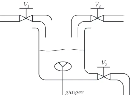
2.1 First Process Control (PROC1)
A simple chemical process frequently considered in literature [9, 16, 17], is initially selected for illustrating the need of FCM learning.
Figure 1 represents the process (PROC1) consisting of one tank and three valves that controls the liquid level in the tank. ValvesV1andV2fill the tank with different liquids. A chemical reaction
takes place into the tank producing a new liquid that leaves the recipient by valveV3. A sensor
(gauger) measures the specific gravity of the resultant mixture.
GAUGER
6 6
6
When the value of the specific gravity,G, is in the range[Gmin, Gmax], the desired liquid has
been produced. The height of the liquid inside, H, must lie in the range [Hmin, Hmax]. The
controller has to keepGandHwithin their bounds,i.e.,
Hmin≤H≤Hmax; (3)
Gmin≤G≤Gmax. (4)
The group of experts defined a list of five concepts, Ci,i = 1, 2, . . . , 5, related to the main
physical quantities of the process, [9].
• ConceptC1: volume of liquid inside the tank (depends onV1,V2, and,V3);
• ConceptC2: state ofV1(closed, open or partially open);
• ConceptC3: state ofV2(closed, open or partially open);
• ConceptC4: state ofV3(closed, open or partially open);
• ConceptC5: specific gravity of the produced mixture.
For this process, the fuzzy cognitive map in Figure 2 can be abstracted [9].
#
#
#
#
#
7
7
7
7
7
7
7
7
Figure 2– Fuzzy Cognitive Map proposed in [9] for the chemical process control problem.
The experts also had a consensus regarding the range of the weights between concepts, as presented in Equations (5) to (12).
−0.50≤W1,2≤ −0.30; (5)
−0.40≤W1,3≤ −0.20; (6)
0.20≤W1,5≤0.40; (7)
0.30≤W2,1≤0.40; (8)
−1.0≤W4,1≤ −0.80; (10)
0.50≤W5,2≤0.70; (11)
0.20≤W5,4≤0.40. (12)
For this problem the following weight matrix is obtained:
W=
⎡
⎢ ⎢ ⎢ ⎢ ⎢ ⎣
0 W1,2 W1,3 0 W1,5
W2,1 0 0 0 0
W3,1 0 0 0 0
W4,1 0 0 0 0
0 W5,2 0 W5,4 0 ⎤
⎥ ⎥ ⎥ ⎥ ⎥ ⎦
. (13)
According to [9], all the experts agreed on range of values forW2,1,W3,1, andW4,1, and most of
them agreed on the same range forW1,2andW1,3. However, regarding the weightsW1,5,W5,2,
andW5,4, their opinions varied significantly.
Finally, the group of experts determined that the values output concepts,C1andC5, which are
crucial for the system operation, must lie, respectively, in the following regions:
0.68≤ A1≤0.70; (14)
0.78≤ A5≤0.85. (15)
2.2 Second Process Control (PROC2)
In [10] a system consisting of two identical tanks with an input and an output valve each one, with the output valve of the first tank being the input valve of the second (PROC2), as illustrated in Figure 3.
6
6
6
4
4
HEATER
Figure 3– PROC2: a chemical process control problem described in [10].
The objective is to control the volume of liquid within the limits determined by the height HminandHmaxand the temperature of the liquid in both tanks within the limitsTminandTmax,
such that
Tmin2 ≤T2≤Tmax2 ; (17)
Hmin1 ≤H1≤Hmax1 ; (18)
Hmin2 ≤H2≤Hmax2 . (19)
The temperature of the liquid in tank 1 is increased by a heater. A thermostat continuously senses the temperature in tank 1, turning the heater on or off. There is also a temperature sensor in tank 2. WhenT2decreases, the valveV2is open and hot liquid comes into tank 2.
Based on this process, a FCM is constructed with eight concepts:
• ConceptC1: volume of liquid inside the tank 1 (depends onV1andV2);
• ConceptC2: volume of liquid inside the tank 2 (depends onV1andV2);
• ConceptC3: state ofV1(closed, open or partially open);
• ConceptC4: state ofV2(closed, open or partially open);
• ConceptC5: state ofV3(closed, open or partially open);
• ConceptC6: Temperature of the liquid in tank 1;
• ConceptC7: Temperature of the liquid in tank 2;
• ConceptC8: Operation of the heater.
According to [10], the fuzzy cognitive map in Figure 4 can be constructed.
It is assumed in this paper only causal constraints in the weights between concepts, where weights W4,1 and W5,2 are ∈ (−1,0] and the others have positive causality. The weight matrix for
PROC2 is given by
W=
⎡
⎢ ⎢ ⎢ ⎢ ⎢ ⎢ ⎢ ⎢ ⎢ ⎢ ⎢ ⎢ ⎣
0 0 W1,3 W1,4 0 0 0 0
0 0 0 W2,4 W2,5 0 0 0
W3,1 0 0 0 0 0 0 0
W4,1 W4,2 0 0 0 0 W4,7 0
0 W5,2 0 0 0 0 0 0
0 0 W6,3 0 0 0 0 W6,8
0 0 0 W7,4 0 0 0 0
0 0 0 0 0 W8,6 0 0
⎤
⎥ ⎥ ⎥ ⎥ ⎥ ⎥ ⎥ ⎥ ⎥ ⎥ ⎥ ⎥ ⎦
. (20)
Finally, it is assumed in this paper that the values output concepts,C1,C2,C6andC7, which are
crucial for the system operation, must lie, respectively, in the following regions:
0.64≤A1≤0.69; (21)
0.63≤ A6≤0.67; (23)
0.63≤ A7≤0.67. (24)
Two significant weaknesses of FCMs are its critical dependence on the experts opinions and its potential convergence to undesired states. In order to handle these impairments, learning pro-cedures can be incorporated, increasing the efficiency of FCMs and avoiding convergence to undesired steady states [18].
#
#
#
#
#
#
#
#
7
7
7
7
7
7
7
7
7
7
7
7
7
Figure 4– Fuzzy Cognitive Map proposed in [10] for the chemical process control problem.
3 METAHEURISTIC FCM LEARNING
In [5] a very interesting survey on FCM learning is provided. The FCM weights optimization (FCM learning) can be classified into three different methods.
1. Hebbian learning based algorithm;
2. Metaheuristic optimization techniques, including genetic algorithm, particle swarm opti-mization, differential evolution, ant colony optimization (these four are population based algorithms), simulated annealing, etc;
3. Hybrid approaches.
In the Hebbian based methodologies, the FCM weights are iteratively adapted based on a law which depends on the concepts behavior [11], [19], requiring the experts’ knowledge for initial weight values. Dickerson and Kosko in [11] proposed the Differential Hebbian Learning (DHL) algorithm, which is a classic example . On the other hand, metaheuristic techniques tries to find a properWmatrix by minimizing a cost function based on the error among the desired values of the output concepts and the current output concepts’ values (27). The experts’ knowledge is not totally necessary, except for the causality constraints, due to the physical restrictions1.
These techniques are optimization tools and generally are computationally complex. Examples of hybrid approaching considering Hebbian learning and Metaheuristic optimization techniques can be found in [20], [21].
According to [22], metaheuristic search methods represent methodologies that can be used in designing underlying heuristics to solve specific optimization problems. PSO, GA and ACO are inside a specific class named population-based metaheuristics.
There are several works in the literature dealing with metaheuristic optimization learning. Most of them are population-based algorithms. For instance, in [9] the PSO algorithm with constriction factor is adopted; in [23] it is presented a FCM learning based on a Tabu Search (TS) and GA combination; in [24] a variation of GA named RCGA (real codec-G.A.) is proposed; in [25] a comparison between GA and Simulated Annealing (SA) is done; in [16] the authors presented a GA based algorithm named Extended Great Deluge Algorithm.
The purpose of the learning is to determine the values of the FCM weights that will produce a desired behavior of the system, which are characterized by theMoutput concept values that lie within desired bounds determined by the experts. Hence, the main goal is to obtain a connection matrix
W=Wi,j, i, j =1,2, . . . , N, (25)
that leads the FCM to a steady state with output concept values within the specified region. Note that, with this notation, and definingA=[A1 · · · AN]⊤, andW=W⊤+I, with{·}⊤meaning
transposition andIidentity matrix, Equation (1) can be compactly written as
A(k+1)= f
W·A(k)
. (26)
After the updating procedure in (26), the following cost function is considered for obtaining the optimum matrixW[9]:
F(W) = M
i=1
HminAiout−Aiout min
Aiout−Aiout +
M
i=1
HAiout−maxAiout max
Aiout−Aiout
, (27)
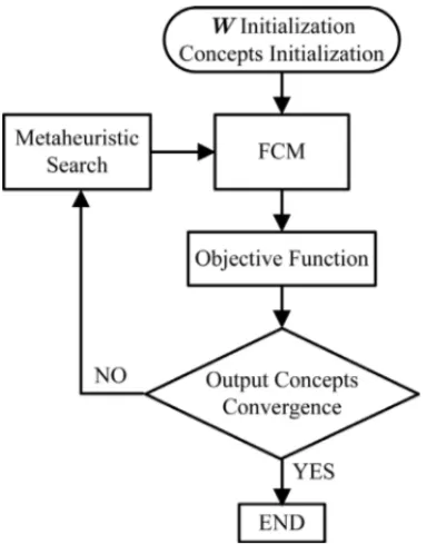
whereH(·)is the Heaviside function, and Aouti ,i =1, . . . , M, represents the value of theith output concept. Figure 5 shows a flowchart of the FCM learning by using metaheuristic search methods.
3.1 Particle Swarm Optimization
Figure 5– Flowchart Fuzzy Cognitive Map learning using metaheuristic search methods.
position of a particle is modified by the application of velocity in order to reach a better per-formance [26, 27]. In PSO, each particle is treated as a point in aW-dimensional space2 and represents a vector-candidate. Theith particle position at instanttis represented as
xi(t)=xi,1(t) xi,2(t) · · · xi,W(t). (28)
In this paper, eachxi,1(t)represents one of theWi,j in thetth iteration. Each particle retains
a memory of the best position it ever encountered. The best position among all particles until thetth iteration (best global position) is represented byxbestg , while the best position of theith particle is represented asxbesti . As proposed in [28], the particles are manipulated according to the following equations:
vi(t+1) = ω·vi(t)+φ1·U1i
xbestg (t)−xi(t)
+φ2·U2i xibest(t)−xi(t)
(29)
xi(t+1) = xi(t)+vi(t+1), (30)
whereφ1andφ2are two positive constants representing the individual and global acceleration
coefficients, respectively,U2i andU2i are diagonal matrices whose elements are random variables uniformly distributed (u.d.) in the interval[0,1], andωis the inertial weight that plays the role of balancing the global search (higherω) and the local search (smallerω).
A typical value forφ1andφ2isφ1=φ2=2 [27]. Regarding the inertia weight, experimental
results suggest that it is preferable to initializeωto a large value, and gradually decrease it.
The populationPsize is kept constant in all iterations. In order to obtain further diversification for the search universe, a factorVmaxis added to the PSO model, which is responsible for limiting
the velocity in the range[±Vmax], allowing the algorithm to escape from a possible local solution.
Regarding the FCM, oneith vector-candidate,xi, is represented by a vector formed byWFCM
weights. It is important to point out that after each particle update, restrictions must be imposed on Wi,j according to the experts opinion, before the cost function evaluation. Algorithm 1 in
Appendix describes the implemented PSO.
3.2 Genetic Algorithm
Genetic Algorithm is an optimization and search technique based on selection mechanism and natural evolution, following Darwin’s theory of species’ evolution, which explains the history of life through the action of physical processes and genetic operators in populations or species. GA allows a population composed of many individuals to evolve under specified selection rules to a state that maximizes the “fitness” (maximizes or minimizes a cost function). Such an algorithm became popular through the work of John Holland in the early 1970s, and particularly his book Adaptation in Natural and Artificial Systems (1975). The algorithm can be implemented in a binary form or in a continuous (real-valued) form. This paper considers the latter case.
Initially, a set of P chromosomes (individuals) is randomly (uniformly distributed) defined, where each chromosome, x consists of a vector of variables to be optimized, which, in this case, is formed by FCM weights, respecting the constraints. Each variable is represented by a continuous floating-point number. ThePchromosomes are evaluated through a cost function.
T strongest chromosomes are selected for mating, generating the mating pool, using the roulette wheel method, where the probability of choosing a given chromosome is proportional to its fitness value. In this paper, each pairing generates two offspring with crossover. The weakest T chromosomes are changed by theT offspring fromT/2 pairing. The crossover procedure is similar to the one presented in [29]. It begins by randomly selecting a variable in the first pair of parents to be the crossover point
α= ⌈u·W⌉, (31)
whereuis a random variable (r.v) u.d. in the interval[0,1], and⌈·⌉is the upper integer operator. A pair of parents is defined as
dad1=xd,1 xd,2 · · · xd,α · · · xd,W
mom1=xm,1 xm,2 · · · xm,α · · · xm,W.
(32)
Then the selected variables are combined to form new variables that will appear in the offspring
xo,1 = xm,α−βxm,α−xd,α;
xo,2 = xd,α+βxm,α−xd,α.
whereβis also a r.v. u.d. in[0,1]. Finally,
offspring1=
xdj,1 xdj,2 xdj,α−1 · · · xoj,1 xmj,α+1· · · xmj,W
offspring2=
xmj,1 xmj,2 xmj,α−1 · · · xoj,2 xdj,α+1· · · xdj,W
.
(34)
In order to allow escaping from possible local minima, a mutation operation is introduced in the resultant population, except for the strongest one (elitism). It is assumed in this work a Gaussian mutation. If the probability of mutations is given by Pm, there will be Nm = ⌈Pm·(P−1)·W⌉mutations uniformly chosen among(P−1)·W variables. Ifxi,wis chosen,
withw=1,2, . . . ,W, than, after Gaussian mutation, it is substituted by
xi,w′ =xi,w+N
0, σm2, (35)
whereN
0, σm2represents a normal r.v. with zero mean and varianceσm2.
After mutation, restrictions must be imposed onWi,j according to the experts opinion, before
the cost function evaluation. Algorithm 2 in Appendix describes the implemented GA.
3.3 Ant Colony Optimization
The Ant Colony Optimization (ACO) metaheuristic was developed to solve optimization prob-lems based on the behavior of ants [30]. These individuals are inserted into a highly structured society, which performs tasks sometimes very complex, for example, the search for food. Dur-ing the search for food, ants release a substance called pheromone, which helps in locatDur-ing the shortest paths from their nest through the food source [30]. The ACO came from this idea, being originally used for solving combinatorial optimization problems.
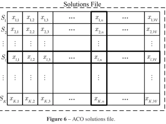
The algorithm implemented in this work is a continuous version of ACO based on the ACOR proposed in [15], where the memory represented by pheromone deposition is substituted by a solutions file.
Initially, a solutions file is created withK candidate solutions, randomly generated. The number of variables of each candidate solution is equal toW. Figure 6 illustrates the configuration of the solutions file.
The solutions file is sorted according to the quality of each solution evaluated through the cost function (fitness), given by (27). Next, for each vector of the solutions file(l=1, . . . ,K), a weightωl is calculated according to the Gaussian function with unitary mean and standard
deviationσ =q K, such that:
ωl =
1
σ√2πe
−(l−2σu2)2
= 1
q K√2πe
−2(lq−21K)22
(36)
1
S
lS
" "Solutions File
1 1,
x
1 2,
x
1 3,
x
1,n
x
1,x
W 2,x
W , lx
W , Kx
W2 1,
x
2 2,
x
2 3,
x
2,n
x
1 , lx
2 , lx
3 , lx
, l nx
1 , Kx
2 , Kx
3 , Kx
, K nx
2S
KS
" " " " " " " " " "Figure 6– ACO solutions file.
A colony with M ants is adopted, which means thatM of the K elements are taken from the solution file to update the position. The roulette wheel method was adopted for choosing the ants, based on a cumulative probability vector with probabilities given by:
pl = ωl K
r=1 ωr
(37)
The next step consists of finding the standard deviation corresponding to each element of a solu-tion vector. Assuming a posisolu-tion (withl =1, . . . ,K,n=1, . . . ,W) of the solution vector, the standard deviation of this element is calculated as:
σl,n = ζ
K −1
K
j=1 j=l
xj,n−xl,n
(38)
whereζ >0, which is also an input parameter, has an effect similar to the evaporation rate of the pheromone in the classical ACO. The convergence speed of the algorithm increases withζ [15]. Thereupon, a Gaussian random variable with zero mean and standard deviationσli is added to a given element of a chosen ant,xl,n, so that new directions are generated for each one of the ants.
Algorithm 3 in Appendix describes the implemented ACO.
4 SIMULATION RESULTS
All simulations were taken considering 104trials for PROC1 and PROC2. The input parameters of the metaheuristic methods were empirically adjusted. For PSO, the first choices wereφ1 = φ2 = 2, ω =1, Vmax = 0 and vi(0)= 0. For GA,T = 2·round(P/4), Pm = 0.1 and σm =0.2 were initially chosen. For ACO,q =0.1 andζ =0.85 were initially tested. However,
4.1 Process PROC1
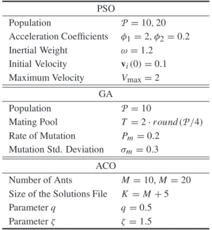
The adopted values for the input parameters of PSO, GA and ACO are summarized on Table 1. Four different scenarios for the process PROC1 were analyzed. The main performance results for each scenario are described in the next subsections.
Table 1– PSO, GA and ACO input parameters values for PROC1. PSO
Population P=10, 20 Acceleration Coefficients φ1=2,φ2=0.2
Inertial Weight ω=1.2 Initial Velocity vi(0)=0.1
Maximum Velocity Vmax=2
GA
Population P=10
Mating Pool T =2·r ound(P/4)
Rate of Mutation Pm=0.2
Mutation Std. Deviation σm=0.3
ACO
Number of Ants M=10,M=20 Size of the Solutions File K=M+5 Parameterq q=0.5 Parameterζ ζ=1.5
4.1.1 Scenario 1
This scenario considers all the constraints on the FCM weights shown in Equations (5) to (12). As mentioned in [9] and also verified here, there is no solution in this case.
4.1.2 Scenario 2
In this scenario, the constraints on the FCM weightsW1,5,W5,2, andW5,4have been relaxed,
since the experts’ opinions have varied significantly. In this case the values of these weights were allowed to assume any value in the interval[0,1]in order to keep the causality of relationships. Tables 2, 3 and 4 present the obtained simulation results for PSO, GA and ACO, respectively.
Table 2– PSO simulation results for Scenario 2, PROC1. PSO withP=10
Amax 0.6882 0.8058 0.6203 0.8389 0.8186
Amin 0.6477 0.7297 0.5749 0.6590 0.7800
Aaverage 0.6840 0.7911 0.6178 0.6713 0.8148
Number of Failures: 49 Probability of Success: 0.9951
PSO withP=20
Amax 0.6882 0.8051 0.6183 0.6967 0.8186
Amin 0.6800 0.7297 0.5750 0.6590 0.7801
Aaverage 0.6838 0.7926 0.6178 0.6730 0.8139
Number of Failures: 0 Probability of Success: 1.0
Table 3– GA simulation results for Scenario 2, PROC1. GA withP=10
Amax 0.6882 0.8051 0.6183 0.6964 0.8186
Amin 0.6800 0.7297 0.5749 0.6590 0.7800
Aaverage 0.6833 0.7726 0.6123 0.6605 0.8059
Number of Failures: 0 Probability of Success: 1.0
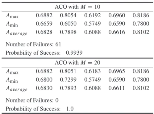
Table 4– ACO simulation results for Scenario 2, PROC1. ACO withM=10
Amax 0.6882 0.8054 0.6192 0.6960 0.8186
Amin 0.6659 0.6050 0.5749 0.6590 0.7800
Aaverage 0.6828 0.7898 0.6088 0.6616 0.8102
Number of Failures: 61 Probability of Success: 0.9939
ACO withM=20
Amax 0.6882 0.8051 0.6183 0.6965 0.8186
Amin 0.6800 0.7299 0.5749 0.6590 0.7800 Aaverage 0.6830 0.7893 0.6088 0.6611 0.8102
0 10 20 30 40 50 0.5 0.55 0.6 0.65 0.7 0.75 0.8 0.85
Number of Iterations
C o n cep t V a lu es C1 C2 C3 C4 C5 (a)
0 10 20 30 40 50
0.5 0.55 0.6 0.65 0.7 0.75 0.8 0.85
Number of Generations
C o n cep t V a lu es C1 C 2 C3 C4 C 5 (b)
0 10 20 30 40 50
0.5 0.55 0.6 0.65 0.7 0.75 0.8 0.85
Number of Iterations
C o n cep t V a lu es C1 C2 C3 C4 C5 (c)
Figure 7– Mean convergence for (a) PSO, (b) GA and (c) ACO in PROC1, Scenario 2 withP=M=10.
0 10 20 30 40 50
0.5 0.55 0.6 0.65 0.7 0.75 0.8 0.85
Number of Iterations
C o n cep t V a lu es C1 C2 C3 C4 C5 (a)
0 10 20 30 40 50
0.5 0.55 0.6 0.65 0.7 0.75 0.8 0.85
Number of Iterations
C o n cep t V a lu es C1 C2 C3 C4 C5 (b)
Figure 8– Mean convergence for (a) PSO and (b) ACO in PROC1, Scenario 2 withP=M=20.
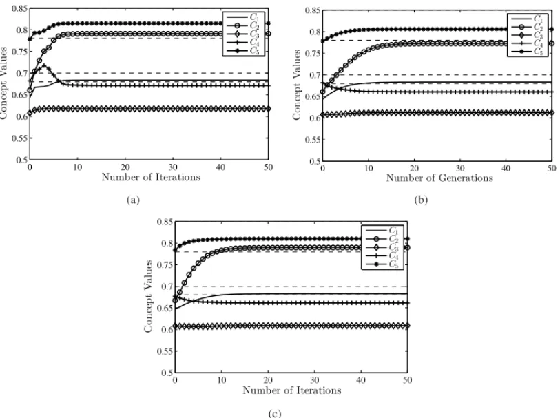
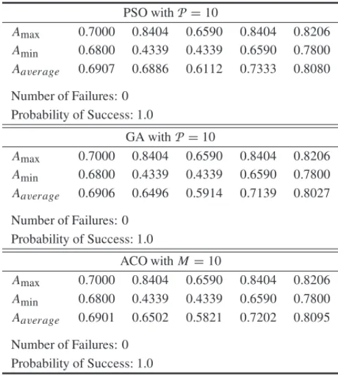
4.1.3 Scenario 3
In this Scenario, all the weights constrains were relaxed, but the causalities were kept,i.e., the value of the weights were fixed in the interval[0,1]or in the interval[−1,0), according to the causality determined by the experts. Table 5 presents the obtained results. As can be seen,
the mean convergence of the concepts in 104independent experiments. In this scenario, the mean convergence speeds were very similar in all cases.
Table 5– GA, PSO and ACO simulation results for Scenario 3, PROC1. PSO withP=10
Amax 0.7000 0.8404 0.6590 0.8404 0.8206
Amin 0.6800 0.4339 0.4339 0.6590 0.7800
Aaverage 0.6907 0.6886 0.6112 0.7333 0.8080
Number of Failures: 0 Probability of Success: 1.0
GA withP=10
Amax 0.7000 0.8404 0.6590 0.8404 0.8206
Amin 0.6800 0.4339 0.4339 0.6590 0.7800
Aaverage 0.6906 0.6496 0.5914 0.7139 0.8027
Number of Failures: 0 Probability of Success: 1.0
ACO withM=10
Amax 0.7000 0.8404 0.6590 0.8404 0.8206
Amin 0.6800 0.4339 0.4339 0.6590 0.7800 Aaverage 0.6901 0.6502 0.5821 0.7202 0.8095
Number of Failures: 0 Probability of Success: 1.0
4.1.4 Scenario 4
In this situation, the causality and the strength of the causality were totally relaxed. The algo-rithms were able to determine proper weights for the connection matrix withP =10. Table 6 presents the obtained statistical results, while Figure 10 presents the mean convergence of the concepts in 104independent experiments. As in Scenario 3, the three schemes presented similar mean convergence speed.
4.2 Process PROC2
For this process the value of the weights were fixed in the interval[0,1]or in the interval[−1,0), according to the causality determined by the experts. The adopted input simulation parameters for PSO, GA and ACO algorithms were the same considered in PROC1, except for the number of ants in ACO that was enough forM =10.
0 10 20 30 40 50 0.5 0.55 0.6 0.65 0.7 0.75 0.8 0.85
Number of Iterations
C o n cep t V a lu es C1 C2 C3 C4 C5 (a)
0 10 20 30 40 50
0.5 0.55 0.6 0.65 0.7 0.75 0.8 0.85
Number of Generations
C o n cep t V a lu es C 1 C2 C3 C4 C5 (b)
0 10 20 30 40 50
0.5 0.55 0.6 0.65 0.7 0.75 0.8 0.85
Number of Iterations
C o n cep t V a lu es C1 C2 C3 C4 C5 (c)
Figure 9– Mean convergence for Scenario 3 in PROC1 considering (a) PSO, (b) GA and (c) ACO with
P= M=10.
Table 6– GA, PSO and ACO simulation results for Scenario 4, PROC1. PSO withP=10
Amax 0.7000 0.9199 0.8206 0.8404 0.8206
Amin 0.6800 0.2129 0.4339 0.3952 0.7800 Aaverage 0.6901 0.6908 0.6767 0.6777 0.8101
Number of Failures: 0 Probability of Success: 1.0
GA withP=10
Amax 0.7000 0.9192 0.8206 0.8404 0.8206
Amin 0.6800 0.2130 0.4339 0.3952 0.7800 Aaverage 0.6905 0.6154 0.6371 0.6306 0.8030
Number of Failures: 0 Probability of Success: 1.0
ACO withM=10
Amax 0.7000 0.9199 0.8206 0.8404 0.8207
Amin 0.6800 0.2129 0.4338 0.3952 0.7800
Aaverage 0.6902 0.5880 0.6215 0.6120 0.8113
0 10 20 30 40 50 0.5 0.55 0.6 0.65 0.7 0.75 0.8 0.85
Number of Iterations
C o n cep t V a lu es C1 C2 C3 C4 C5 (a)
0 10 20 30 40 50
0.5 0.55 0.6 0.65 0.7 0.75 0.8 0.85
Number of Generations
C o n cep t V a lu es C1 C2 C3 C4 C5 (b)
0 10 20 30 40 50
0.5 0.55 0.6 0.65 0.7 0.75 0.8 0.85
Number of Iterations
C o n cep t V a lu es C1 C2 C3 C4 C5 (c)
Figure 10– Mean convergence for Scenario 4 in PROC1 considering (a) PSO, (b) GA and (c) ACO with
P=M=10.
30 failures and probability of success equal to 0.9970. However, withP = 20, PSO was able to achieve 100% of success. For this process, PSO has a faster average convergence than GA and ACO.
Table 8 shows the mean execution time in 50 iterations for each algorithm in all considered configuration. A computer with CPU Intel Core i7-2675QM @ 2.20GHz and 6GB of RAM was considered. As can be seen, the way the algorithms were implemented, PSO has a execution time shorter than GA and ACO, being ACO the slowest scheme.
5 CONCLUSIONS
Fuzzy cognitive maps have being considered with great interest in a large range of applica-tions. Learning methods may be necessary for obtaining proper values for the weight matrix and reducing the dependence on the experts’ knowledge.
Table 7– GA, PSO and ACO simulation results for PROC2. PSO withP=10
Amax 0.7040 0.6590 0.9029 0.9407 0.8134 0.7234 0.6700 0.8153
Amin 0.6400 0.4130 0.6590 0.6590 0.6590 0.6590 0.6590 0.6590 Aaverage 0.6592 0.5006 0.7079 0.7221 0.6809 0.6593 0.6592 0.6850
Number of Failures: 30 Probability of Success: 0.9970
PSO withP=20
Amax 0.6800 0.5200 0.9040 0.9411 0.7869 0.6700 0.6700 0.8154
Amin 0.6400 0.4800 0.6590 0.6590 0.6590 0.6590 0.6590 0.6590
Aaverage 0.6594 0.5002 0.7116 0.7267 0.6813 0.6594 0.6593 0.6865
Number of Failures: 0 Probability of Success: 1.0
GA withP=10
Amax 0.6800 0.5200 0.9038 0.9409 0.7870 0.6700 0.6700 0.8153
Amin 0.6400 0.4800 0.6590 0.6590 0.6590 0.6590 0.6590 0.6590
Aaverage 0.6596 0.5014 0.7500 0.7717 0.7055 0.6596 0.6596 0.7082
Number of Failures: 0 Probability of Success: 1.0
ACO withM=10
Amax 0.6800 0.5200 0.9049 0.9415 0.7870 0.6700 0.6700 0.8154
Amin 0.6400 0.4800 0.6590 0.6590 0.6590 0.6590 0.6590 0.6590
Aaverage 0.6595 0.4997 0.7674 0.7938 0.7045 0.6604 0.6604 0.7170
Number of Failures: 0 Probability of Success: 1.0
Table 8– Execution time.
Process Algorithm Population Time (ms) PROC. 1 PSO P=10 16.6 PROC. 1 PSO P=20 30.4
PROC. 1 GA P=10 21.6
PROC. 1 ACO M=10,K =15 45.4 PROC. 1 ACO M=20,K =25 94.9 PROC. 2 PSO P=10 17.2 PROC. 2 PSO P=20 33.0
PROC. 2 GA P=10 22.9
0 10 20 30 40 50 0.45 0.5 0.55 0.6 0.65 0.7 0.75 0.8
Number of Iterations
C o n cep t V a lu es C1 C2 C3 C4 C5 C6 C7 C8 (a)
0 10 20 30 40 50
0.45 0.5 0.55 0.6 0.65 0.7 0.75 0.8
Number of Generations
C o n cep t V a lu es C1 C2 C3 C4 C5 C6 C7 C8 (b)
0 10 20 30 40 50
0.45 0.5 0.55 0.6 0.65 0.7 0.75 0.8
Number of Iterations
C o n cep t V a lu es C1 C2 C3 C4 C5 C6 C7 C8 (c)
0 10 20 30 40 50
0.45 0.5 0.55 0.6 0.65 0.7 0.75 0.8
Number of Iterations
C o n cep t V a lu es C1 C2 C3 C4 C5 C6 C7 C8 (d)
Figure 11– Mean convergence in PROC2 for (a) PSO withP =10, (b) GA withP=10, (c) ACO with M=10 and (d) PSO withP=20.
to the other two schemes, being ACO the second best technique in terms of probability of success in the two considered processes (somewhat better than PSO).
Specially in scenario 2 of PROC 1, when there are several weight constraints, GA achieved 100% of success in 104independent experiments with a population of 10 chromosomes. PSO and ACO neededP =20 particles andM =20 ants in the population in order to reach 100% of success. In PROC2, both GA and ACO neededP = M =10, while PSO presented only 30 failures in 104independent experiments whenP=10, and no errors whenP=20.
In terms of execution time in 50 iterations and considering the input parameters adopted, ACO presented the slowest time, being PSO the fastest algorithm. It is important to emphasize that no code optimization techniques have been considered while implementing PSO, GA and ACO.
REFERENCES
[1] KOSKOB. 1986. Fuzzy cognitive maps.International Journal of Man-Machine Studies,24: 65–75. [2] KOSKOB. 1992. Neural networks and fuzzy systems: a dynamical systems approach to machine
intelligence. Prentice Hall, Upper Saddle River, NJ.
[3] KOSKOB. 1997. Fuzzy Engineering. Prentice-Hall, Inc., Upper Saddle River, NJ.
[4] AXELROD RM. 1976. Structure of Decision: The Cognitive Maps of Political Elites. Princeton University Press, Princeton, NJ.
[5] PAPAGEORGIOUEI. 2012. Learning algorithms for fuzzy cognitive maps – a review study.IEEE Transactions on Systems, Man, and Cybernetics– Part C,42(2): 150–163.
[6] ANDREOUAS, MATEOUNH & ZOMBANAKISGA. 2005. Soft computing for crisis management and political decision making: the use of genetically evolved fuzzy cognitive maps.Soft Computing, 9: 194–210.
[7] STYLIOSCD, GEORGOPOULOSVC, MALANDRAKIGA & CHOULIARAS. 2008. Fuzzy cognitive map architectures for medical decision support systems.Applied Soft Computing,8: 1243–1251. [8] PAPAGEORGIOUEI, STYLIOSCD & GROUMPOSPP. 2003. An integrated two-level hierarchical
system for decision making in radiation therapy based on fuzzy cognitive maps.IEEE Transactions on Biomedical Engineering,50(12): 1326–1339.
[9] PAPAGEORGIOUEI, PARSOPOULOSKE, STYLIOSCS, GROUMPOSPP & VRAHATISMN. 2005. Fuzzy cognitive maps learning using particle swarm optimization.Journal of Intelligent Information Systems,25: 95–121.
[10] STYLIOSCD, GEORGOPOULOSVC & GROUMPOSPP. 1997. The use of fuzzy cognitive maps in modeling systems. In: Proceeding of 5thIEEEMediterranean Conference on Control and Systems, Paphos.
[11] DICKERSONJA & KOSKOB. 1993. Virtual worlds as fuzzy cognitive maps. In:IEEE Virtual Reality Annual International Symposium,3: 471–477.
[12] TABERR. 1991. Knowledge Processing With Fuzzy Cognitive Maps.Expert Systems With Applica-tions,1(2): 83–87.
[13] PERUSICHK. 1996. Fuzzy cognitive maps for policy analysis. In: International Symposium on Tech-nology and Society Technical Expertise and Public Decisions, pages 369–373.
[14] PAPAGEORGIOUEI & SALMERONJL. 2013. A review of fuzzy cognitive maps research during the last decade.IEEE Transactions on Fuzzy Systems,21(1): 66–79.
[15] SOCHAK & DORIGOM. 2008. Ant colony optimization for continuous domains.European Journal of Operational Research,185(3): 1155–1173.
[16] BAYKASOGLUA, DURMUSOGLUZDU & VAHITK. 2011. Training fuzzy cognitive maps via ex-tended great deluge algorithm with applications.Computers in Industry,62(2): 187–195.
[17] GLYKASM. 2010. Fuzzy Cognitive Maps: Advances in Theory, Methodologies, Tools and Applica-tions. 1stedition, Springer Publishing Company, Incorporated.
[18] PARSOPOULOSKE & GROUMPOSPP. 2003. A first study of fuzzy cognitive maps learning using particle swarm optimization. In: IEEE 2003 Congress on Evolutionary Computation, pages 1440– 1447.
[20] PAPAGEORGIOUEI & GROUMPOSPP. 2005. A new hybrid learning algorithm for fuzzy cognitive maps learning.Applied Soft Computing,5: 409–431.
[21] ZHUY & ZHANGW. 2008. An integrated framework for learning fuzzy cognitive map using rcga and nhl algorithm. In: Int. Conf. Wireless Commun., Netw. Mobile Comput., Dalian, China. [22] TALBIE-G. 2009. Metaheuristics – From Design to Implementation. 1st edition, Wiley, Hoboken,
NJ, USA.
[23] ALIZADEHS, GHAZANFARIM, JAFARIM & HOOSHMANDS. 2007. Learning fcm by tabu search. International Journal of Computer Science,3: 142–149.
[24] STACHW, KURGANLA, PEDRYCZW & REFORMATM. 2005. Genetic learning of fuzzy cognitive maps.Fuzzy Sets and Systems,153(3): 371–401.
[25] GHAZANFARIM, ALIZADEHS, FATHIANM & KOULOURIOTISDE. 2007. Comparing simulated annealing and genetic algorithm in learning fcm.Applied Mathematics and Computation,192(1): 56–68.
[26] KENNEDYJ & EBERHARTR. 1995. Particle swarm optimization. In: IEEE International Conference on Neural Networks, pages 1942–1948.
[27] KENNEDYJ & EBERHARTRC. 2001. Swarm Intelligence. 1stedition, Morgan Kaufmann. [28] SHIY & EBERHARTRC. 1998. A modified particle swarm optimizer. In: IEEE International
Con-ference on Evolutionary Computation, pages 69–73.
[29] HAUPTRL & HAUPTSE. 2004. Practical Genetic Algorithms. 2nd edition, John Wiley & Sons, Hoboken, NJ, USA.
[30] DORIGOM & ST¨UTZLET. 2004. Ant Colony Optimization. 1stedition, Bradford Book, Hoboken, NJ, USA.
APPENDIX
Algorithm 1PSO FCM LEARNING
Input: P,G,ω,Vmax,vi(0),φ1,φ2,Vmax,Wmin,Wmax,Amin,Amax Output: Wopt
Initialize first population (randomly generated) of weights∈[Wmin,Wmax];
Initial Evaluation through cost function (Equation (27));
Find best global and best individual positions (initialy,xbestg =xbesti ); while(t ≤Gor output concepts convergence):
a. update velocityvi(t+1), i =1, . . . ,P, through (29);
b. velocity limitation byVmax;
c. update positionxi(t+1), i =1, . . . ,P, through (30);
d.x(i.e.,W) limitation∈ [Wmin;Wmax];
e. Evaluation through cost function (Eq. (27));
f. Find best global (xbestg ) and best individual positions (xbesti ); end
− − − − − − − − − − − − − − − − − − − − − − − − − − − − − − − − − − − − − − − Wmin,Wmax: matrices of weights (particle positions) constraints;
Algorithm 2GA FCM LEARNING
Input: P,G,T,Pm,σm,Wmin,Wmax,Amin,Amax Output: Wopt
Initialize first population (randomly generated) of weights∈[Wmin,Wmax];
Initial Evaluation through cost function (Eq. (27)); while(t≤Gor output concepts convergence):
a. Selection ofT individuals: roulette wheel for selecting chromosomes; b. Pairing and crossover (Eq. (31) to (34));
c. Gaussian Mutation (Eq. 35);
d.x(i.e.,W) limitation∈ [Wmin;Wmax];
d. Evaluation through cost function (Eq. (27)); e. SortWand update best result;
end
− − − − − − − − − − − − − − − − − − − − − − − − − − − − − − − − − − − − − − − Wmin,Wmax: matrices of weights (particle positions) constraints;
Amin,Amax: matrices of concepts constraints; Wopt: optimum weight matrix.
Algorithm 3ACO FCM LEARNING
Input: M,K,q,ζ,G,Wmin,Wmax,Amin,Amax Output:Wopt
Initialize solutions file (randomly generated) of weights∈[Wmin,Wmax];
Initial Evaluation through cost function (Eq. (27)); Sort solutions file according to the fitness;
Calculateωl(Eq. (36)) and pl(Eq. (37));
while(t≤Gor output concepts convergence):
a. Selection ofMants: roulette wheel according to pl;
b. Calculateσl,n(Eq. (38));
c. Update ants position (xl,n) adding aN(0, σl,n)variable to the previous position;
d.x(i.e.,W) limitation∈ [Wmin;Wmax];
d. Evaluation through cost function (Equation (27)); e. SortWand update best result;
end
− − − − − − − − − − − − − − − − − − − − − − − − − − − − − − − − − − − − − − − Wmin,Wmax: matrices of weights (particle positions) constraints;
![Figure 2 – Fuzzy Cognitive Map proposed in [9] for the chemical process control problem.](https://thumb-eu.123doks.com/thumbv2/123dok_br/18870984.420081/4.1063.310.697.740.1045/figure-fuzzy-cognitive-proposed-chemical-process-control-problem.webp)
![Figure 3 – PROC2: a chemical process control problem described in [10].](https://thumb-eu.123doks.com/thumbv2/123dok_br/18870984.420081/5.1063.294.968.144.469/figure-proc-chemical-process-control-problem-described-in.webp)
![Figure 4 – Fuzzy Cognitive Map proposed in [10] for the chemical process control problem.](https://thumb-eu.123doks.com/thumbv2/123dok_br/18870984.420081/7.1063.349.780.378.702/figure-fuzzy-cognitive-proposed-chemical-process-control-problem.webp)