Single Photon Emission Mammography with
Convergent Collimators
Doutoramento em Engenharia Biomédica e Biofísica
Ricardo Miguel Ferreira Capote
Tese orientada por:
Prof. Doutor Pedro Dinis de Almeida
Documento especialmente elaborado para a obtenção do grau de doutor
Single Photon Emission Mammography with
Convergent Collimators
Doutoramento em Engenharia Biomédica e Biofísica
Ricardo Miguel Ferreira Capote
Tese orientada por:
Prof. Doutor Pedro Dinis de Almeida
Júri:Presidente:
• Doutora Margarida Maria Telo da Gama Vogais:
• Doutor Stefaan Vandenberghe
• Doutor Nuno David de Sousa Chichorro da Fonseca Ferreira • Doutor Luís Manuel de Almeida Soares Janeiro
• Doutora Mónica Vieira Martins
• Doutor João Manuel Coelho dos Santos Varela • Doutor Pedro Miguel Dinis de Almeida • Doutor Nuno Miguel de Pinto Lobo e Matela
Documento especialmente elaborado para a obtenção do grau de doutor
To those who dedicate their lives to scientific research and share their knowledge without expecting anything in return.
Since the beginning of my PhD, there has been an alarming increase in the number of things I know nothing about…
I would like to express my gratitude to those who have contributed to this PhD thesis. The comments are written in my mother tongue, Portuguese.
Professor Pedro Almeida Por ter acreditado e confiado nas minhas capacidades para realizar este trabalho. Pela orientação, amizade e por ter apoiado e encorajado a desenvolver novas ideias.
Professor Nuno Matela Pela amizade e por ter sido um apoio constante a nível profissional e pessoal. Pelo tempo prestado em todas as discussões e lições que contribuíram para a realização desta tese.
Beatriz Lampreia Pelo carinho, amizade e alegria contagiante. Por estar sempre disponível para ajudar e por tornar o IBEB num local especial.
Staff do Instituto de Engenharia Biomédica e Biofísica Pela boa disposição e simpatia: Professor Alexandre Andrade, Professor Eduardo Ducla-Soares, Professor Hugo Ferreira e Professor Pedro Miranda.
Colegas do Instituto de Engenharia Biomédica e Biofísica Pela ajuda e por todos os momentos proporcionados que guardo com saudade: Nuno Oliveira, Liliana Caldeira, Cláudia Sofia Ferreira, Raquel Conceição, Bárbara Oliveira, Ricardo Salvador, Rita Nunes, Margarida Mota, João Rodrigues, Cornelia Wenger, Pedro Barata, Ana Teixeira, e muitos outros que passaram pelo IBEB. Ao Gilberto de Almeida e Ana Carina de Oliveira pela ajuda na fase inicial deste trabalho.
Colegas do Projeto Clear-PEM e Crystal Clear Collaboration Pela ajuda e pela integração no projeto.
Colegas da FCUL Com quem colaborei na docência. Em especial ao Professor João Lin pela amizade e palavras de encorajamento; e à Professora Margarida Pires por toda ajuda.
Meus amigos A todos os meus amigos de longa data, que me proporcionam momentos de diversão e alegria.
Minha Família Aos meus pais e irmão por todo o amor, carinho e por sempre me terem motivado a dar o meu melhor e a atingir os meus objectivos.
Margarida Inácio Por todo amor e apoio. Por me compreender para além das palavras. Pela capacidade de superar as adversidades da vida. Por me fazer feliz.
À memória do meu avô Capote, Pelo altruísmo e preocupação constante com os netos. Por me incentivar a estudar e a ambicionar um futuro melhor.
À memória de Natália Inácio, Pelo carinho, força e pelo sorriso meigo com que sempre me recebeu. Por partilhar conselhos sensatos e encarar a vida com uma atitude de superação.
This work was financed in part by the Fundação para a Ciência e Tecnologia (FCT) under the PhD grant SFRH/BD/47075/2008 and the strategic plan of the Instituto de Biofísica e Engenharia Biomédica (PEst-OE/SAU/UI0645/2011).
De acordo com as estatísticas mundiais, nas mulheres, o cancro da mama é a neoplasia mais comum e corresponde à segunda causa de morte por cancro. A detecção e diagnóstico precoce desempenham um papel fundamental no sucesso do tratamento e melhoria das taxas de sobrevivência dos doentes. Por este motivo, as técnicas de diagnóstico por imagem têm sido desenvolvidas e melhoradas ao longo dos últimos anos.
Atualmente, a mamografia por raios X é a técnica standard usada nos rastreios do cancro da mama. Os programas de rastreio permitem um diagnóstico mais precoce e têm contribuído, em simultâneo com as melhorias do tratamento, para a diminuição da mortalidade por cancro da mama. No entanto, a mamografia por raios X fornece informação essencialmente anatómica e a sensibilidade do exame é reduzida, especialmente em mulheres com tecido mamário denso. Desta forma, é necessário recorrer a outras técnicas que permitam obter informação adicional sobre os tumores detectados e reduzir o número de procedimentos invasivos desnecessários, como as biopsias.
As técnicas de Medicina Nuclear, nomeadamente a tomografia por emissão de positrões (PET) ou a tomografia computorizada por emissão de fotão único (SPECT), são frequentemente utilizadas como técnicas de diagnóstico complementar. Estas técnicas permitem uma avaliação precisa da presença e extensão da doença e obtêm informação única sobre as características biológicas do tumor (como a taxa de proliferação e atividade metabólica). Por estas razões, na última década foram desenvolvidos equipamentos específicos para mamografia. Os equipamentos de mamografia por emissão de fotão único (SPEM) e mamografia por emissão de positrões (PEM) permitem obter melhor sensibilidade e resolução espacial que os equipamentos PET ou SPECT para exames de corpo inteiro.
O scanner Clear-PEM é um equipamento PEM que foi desenvolvido pelo Consórcio Português PET-Mamografia e permite detectar pequenos tumores (aproximadamente com 2 mm) da mama nos seus estágios iniciais. O scanner contém duas cabeças detectoras que são colocadas junto da mama, permitindo a detecção da radiação emitida pelo radiofármaco previamente injetado no doente. No entanto, a atual geometria de aquisição só permite a detecção de coincidências nas quais a aniquilação do positrão ocorreu na região entre as cabeças detectoras. De facto, as coincidências (par de fotões com aproximadamente 180°) emitidas a partir de posições fora desta região não
produzem uma linha de resposta detectável. Portanto, os tumores localizados em regiões acima das cabeças detectoras não são detectados. Estas regiões incluem a zona axilar e do arco costal, que são zonas importantes para o diagnóstico do cancro da mama. Esta limitação resulta na visualização de uma imagem incompleta ou truncada do volume mamário. A limitação em detectar tumores localizados no arco costal ou zona axilar é também comum nos equipamentos SPEM que usam colimadores convencionais (colimadores paralelos que são normalmente orientados com os orifícios perpendiculares ao eixo central da mama). Desta forma, este assunto tem sido objecto de diversos estudos, realizados pela comunidade científica, e foram propostas algumas soluções.
Nesta tese, apresentamos uma solução para a referida limitação dos equipamentos SPEM e demonstramos a sua viabilidade. Dado que este trabalho foi desenvolvido no âmbito do projeto Clear-PEM, pretendeu-se também investigar a viabilidade de usar o scanner Clear-PEM em modo singles (ou modo SPECT) para examinar a região do arco costal. Desta forma, a solução encontrada foi adaptada às características do scanner Clear-PEM. Em ambos os casos, pretendeu-se obter uma solução capaz de detectar tumores com elevada resolução espacial (2-3 mm) e com valores de sensibilidade comparáveis aos dos equipamentos clínicos de SPECT (0.01-0.03%).
A solução apresentada é baseada na geometria de colimação cone beam, cujos orifícios do colimador são inclinados em direção às regiões da mama e arco costal. Esta solução é mais simples e eficiente comparativamente às do estado de arte. Com o objectivo de maximizar a sensibilidade do colimador para um valor fixo de resolução espacial, desenvolvemos um algoritmo para a optimização de colimadores convergentes. Este algoritmo foi utilizado na projeção de colimadores optimizados para dois equipamentos diferentes: um scanner genérico de SPEM e o scanner Clear-PEM.
A validação e estudo da performance de ambos equipamentos com os respectivos colimadores foi efectuada com recurso a simulações Monte-Carlo (foi utilizada a plataforma de simulação GATE). Em ambos os casos, foram utilizados os seguintes parâmetros de simulação: detectores pixelizados com espaçamento mínimo entre cristais de 2.3 mm, colimadores de tungsténio, janela de energia entre 120-160 keV, adquiridas 128 projeções ao longo de uma órbita de aquisição circular com 5 cm de raio, tempos de aquisição de 11-21 minutos, e fantômas com discos uniformes (fantôma Defrise) e de resolução (fantôma Derenzo). Foi também simulado um exame clínico real utilizando o fântoma realístico XCAT para modelar a mama, torso e respectivos órgãos.
O algoritmo iterativo Maximum Likelihood Expectation Maximization (MLEM) foi implementado e utilizado na reconstrução dos dados simulados. A função de resposta de cada sistema foi simulada e incorporada no processo de reconstrução. Desta forma, foram incluídos no algoritmo os principais efeitos físicos e geométricos. As imagens foram
reconstruídas com um tamanho de voxel de 1 mm3 e não foram utilizados filtros nem
foram aplicadas correções.
Para ambos os casos, os resultados demonstraram a presença de artefactos na imagem, devido ao facto de a geometria cone beam e a órbita de aquisição utilizada não permitirem uma amostragem completa dos dados simulados. No entanto, foi possível detectar tumores de 3 mm localizados na região do arco costal e provar a viabilidade da solução. As imagens com melhor qualidade foram obtidas com o scanner SPEM. Diferentes restrições técnicas (relacionadas com a adaptação para aquisições em modo singles) comprometeram os resultados obtidos com o scanner Clear-PEM.
Os colimadores propostos nesta tese permitem examinar a mama e o arco costal, obtendo informação de diagnóstico adicional. Esta geometria de colimação tem um elevado potencial para ser utilizada em exames a pequenos órgãos (como o cérebro ou coração) ou pequenos animais.
Palavras-Chave: Cancro da Mama, Mamografia por Emissão de Fotão Único, Colimador Cone Beam, Optimização de Colimadores, Reconstrução de Imagem SPECT.
The radionuclide based imaging techniques offer substantial potential as complementary diagnostic tools. Dedicated radionuclide systems for breast cancer imaging have been intensively investigated over the past decade. However, these breast-specific systems cannot image the chest wall region. The aim of this work is to present a solution to solve this imaging limitation and demonstrate its feasibility.
The proposed solution is based on the cone beam collimation geometry, whose collimator holes are angled toward the breast and chest regions. It is shown that this approach is simpler and more efficient compared to other state of the art approaches. In order to maximize the collimator sensitivity for a fixed spatial resolution, we developed an optimization algorithm for convergent collimators. This algorithm was used to project optimal collimators for two different systems: a single-photon emission mammography (SPEM) scanner and the positron emission mammography (PEM) scanner developed by the Clear-PEM project.
Monte Carlo simulations were performed to study the expected performance of both scanners with the respective collimators. The main simulated parameters include: 2.3 mm detector pixels, tungsten collimators, 120-160 keV energy window, 128 step-and-shoot projections acquired over a 5 cm radius circular orbit, acquisition times of 11-21 minutes, and uniform disc (Defrise) and resolution (Derenzo) phantoms filled with Tc-99m. We also simulated a real clinical exam using a realistic breast (XCAT) phantom.
The simulated data were reconstructed using an iterative maximum likelihood expectation maximization algorithm (MLEM) with 1 mm3 voxels and each system
response was included in the reconstruction process.
Overall, due to technical challenges involved in the adaptation of the Clear-PEM to single-photon acquisitions, the best results were obtained with the SPEM scanner. The proposed collimators offer enhanced diagnostic information by detecting down to 3 mm chest wall lesions and have a great potential for use in small field of view applications.
Keywords: Breast Cancer; Single Photon Emission Mammography, Cone Beam Collimator, Collimator Optimization, SPECT Image Reconstruction.
Acknowledgments ... v
!
Resumo ... vii
!
Abstract ... xi
!
Contents ... xiii
!
List of Figures ... xvii
!
List of Tables ... xxv
!
Acronyms and Abbreviations ... xxvii
!
Part I: Introduction and Background ... 1
!
1
!
Introduction ... 3!
2
!
Breast Cancer Imaging ... 7!
2.1! Introduction ... 7!
2.1.1! X-ray mammography ... 9!
2.1.2! Magnetic Resonance Imaging ... 9!
2.1.3! Ultrasound imaging ... 10!
2.1.4! Radionuclide imaging ... 11!
2.1.5
!
Other imaging modalities ... 12!
2.2
!
Single Photon Emission Mammography ... 13!
2.2.1! Detector ... 15!
2.2.2! Collimator ... 18!
2.2.3! Commercial SPEM scanners ... 21!
2.2.4! SPECT systems for breast and chest wall imaging ... 23!
2.3! Positron Emission Mammography ... 25!
2.3.1! Commercial PEM scanners ... 27!
2.3.2! Clear-PEM scanner ... 28!
2.4! Dual modality PET/SPECT systems ... 31!
2.4.1! Advantages ... 31!
2.4.2! Challenges ... 31!
2.4.3! Research PET/SPECT systems ... 32!
2.5! Conclusions ... 33!
3
!
Projection and Collimator Optimization ... 37!
3.1! Introduction ... 37!
3.2! FOV required to image the breast ... 38!
3.3! Choosing the collimation geometry ... 39!
3.3.1
!
Cone beam vs. Pinhole ... 40!
3.4! Convergent collimator theory ... 42!
3.4.1! Fan beam geometry ... 43!
3.4.2! Cone beam geometry ... 45!
3.4.3! Average efficiency ... 46!
3.4.4
!
Collimator near-field considerations ... 47!
3.4.5! Collimator mass ... 48!
3.4.6! Collimator design with multiplexing ... 49!
3.5! Optimization method for converging collimators ... 53!
3.5.1! Methods ... 55!
3.5.2! Optimal hole dimensions: dependence on the hole incidence angle ... 57!
3.5.3! Optimal collimator dimensions: dependence on the focal distance ... 60!
3.5.4! Optimal collimators for use in small FOV applications ... 63!
3.5.5! General discussion of the optimization method ... 65!
3.6! Optimal collimators for breast and chest wall imaging ... 67!
3.6.1! Optimal collimators for a SPEM scanner ... 67!
3.6.2! Optimal collimators for the Clear-PEM scanner ... 71!
3.6.3! Final considerations and discussion ... 73!
3.7
!
Conclusions ... 75!
4
!
Monte Carlo Simulations ... 77!
4.1! Introduction ... 77!
4.2! Monte Carlo simulations ... 77!
4.2.1! GATE toolkit ... 78!
4.2.2! Phantom ... 79!
4.3
!
SPEM scanner simulation framework ... 80!
4.3.1
!
Detector geometry ... 80!
4.3.2! Collimator geometry ... 81!
4.3.3! Digitizer parameters ... 82!
4.3.4! Physics and other parameters ... 83!
4.4! Clear-PEM scanner simulation framework ... 84!
4.4.1! Detector geometry ... 84!
4.4.2! Collimator geometry ... 85!
4.4.3! Digitizer parameters ... 86!
4.4.4! Physics and other parameters ... 86!
4.4.5! Simulation of LYSO:Ce background ... 86!
4.5! Simulated Phantoms ... 88!
4.5.1! Derenzo phantom ... 88!
4.5.2! Defrise phantom ... 89!
4.5.3! XCAT phantom ... 89!
4.6.1! SPEM scanner results ... 94!
4.6.2! Clear-PEM scanner results ... 94!
4.6.3! Discussion ... 96!
4.7! Simulation of the system response function ... 97!
4.7.1! SPEM scanner results ... 98!
4.7.2! Clear-PEM scanner results ... 99!
4.7.3! Discussion ... 100!
4.8! Conclusion ... 100!
5
!
SPECT Image Reconstruction ... 103!
5.1! Introduction ... 103!
5.2! Image reconstruction ... 103!
5.2.1! MLEM algorithm ... 105!
5.2.2! System matrix ... 106!
5.2.3! Cone beam reconstruction: data sampling ... 107!
5.3! Methods ... 109!
5.3.1
!
Image reconstruction ... 109!
5.3.2
!
Image analysis ... 109!
5.4! Reconstructed images from simulated data ... 110!
5.4.1! SPEM scanner results ... 111!
5.4.2! Clear-PEM scanner results: without the LYSO:Ce background ... 116!
5.4.3! Discussion ... 120!
5.5! Conclusion ... 121!
Part III: General Conclusion ... 123
!
6
!
Main Conclusions and Future Work ... 125!
6.1! Conclusion ... 125!
6.1.1! Projection and collimator optimization ... 126!
6.1.2! Monte Carlo simulations ... 127!
6.1.3
!
SPECT image reconstruction ... 129!
6.2! Concluding Remarks ... 130!
6.3! Main goals achieved ... 131!
6.4! Future Work ... 131!
Bibliography ... 133
!
Appendix A: Images of the simulation framework (GATE) ... 147
!
Appendix B: Simulated projection data ... 149
!
Figure 1.1 – Diagram showing the thesis structure and the main topics. ... 6
!
Figure 2.1 – Incidence rates and death rates among females for selected cancers, UnitedStates, 1975 to 2009: (a) Incidence rates and (b) Death rates (Uterus includes uterine cervix and uterine corpus). Adapted from [17]. ... 7
!
Figure 2.2 – Illustration showing the anatomy of the female breast. The nipple and theareola are shown on the outside of the breast. The axillary lymph nodes network, ducts, lobules and other parts of the inside of the breast are also shown (Adapted from [19]). ... 8
!
Figure 2.3 - Diagram showing the information provided by each medical imaging modalitybased on its widespread use. Note that based on the widespread use of the breast imaging modalities both x-ray mammography and breast US provide mainly anatomical information, however it was considered their ability to provide functional information about the breast tissues. ... 11
!
Figure 2.4 - Illustration showing the selective absorption performed by a parallel holecollimator. A gamma photon (green arrow) that passes through the collimator reaching the detector and a photon that is absorbed by the collimator septa (blue lines) are shown. ... 13
!
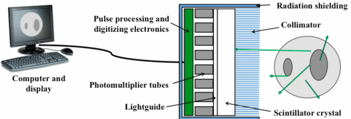
Figure 2.5 - Illustration showing the fundamental components of a conventional gammacamera. The basic structure of the Anger Camera comprises a collimator, scintillator crystal, light guide that allows light to spread, an array of photomultiplier tubes with related electronics, a radiation shielding, a computer and display for acquisition, processing and display of data and images. The circular shape at the right and the green lines represent the object being imaged and the emitted gamma rays, respectively. ... 14
!
Figure 2.6 - Illustration showing the light ray propagation for: (a) single continuous crystaland (b) discrete crystal camera designs. For the pixelated design, the scintillation light is confined to one crystal and focused onto a small spot on the photo detector array. The collimator, scintillation crystals and position-sensitive photodetector are shown. The approximate shapes of the resulting response functions for each case are indicated. The green and black lines represent the detected gamma rays and optical scintillation rays, respectively. ... 15
!
Figure 2.7 - Illustration showing the calculation of the energy resolution for Tc-99m 140 keVgamma rays. The shaded area corresponds to the energy window that is used to select a range of acceptable photon energies. For example, a window setting of 20% for the 140 keV photopeak corresponds to a 28 keV range centred on 140 keV (126 keV to 154 keV). ... 17
!
Figure 2.8 - Illustration showing the different collimation geometries: (a) Parallel hole collimator, (b) Slant hole collimator, (c) Diverging collimator, (d) Converging collimator and (e) Pinhole collimator. ... 18
!
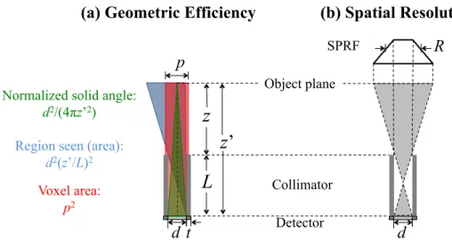
Figure 2.9 – Definition of both performance parameters of the collimator, based on theSPRF: (a) geometric efficiency, including the illustration of the 3 factors used in the calculation; and (b) spatial resolution, which is defined as the FWHM of the SPRF (2D view). ... 21
!
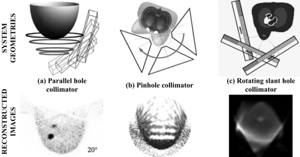
Figure 2.10 – Illustration of the different documented approaches that permit to detectlesions in both breast and chest wall regions: (a) system with parallel hole collimator coupled to a tiltable head (above) and reconstructed breast image for a tilting angle of 20º (below), (b) system with pinhole collimator coupled to a tiltable head (above) and reconstructed image of a breast phantom with cold disks (below), and (c) system with rotating slant hole collimator coupled to a tiltable head (above) and reconstructed breast image (below). Adapted from [8,10,14]. ... 24
!
Figure 2.11 – Illustration showing the detection of both annihilation photons. The line atgreen represents the Line of Response. ... 26
!
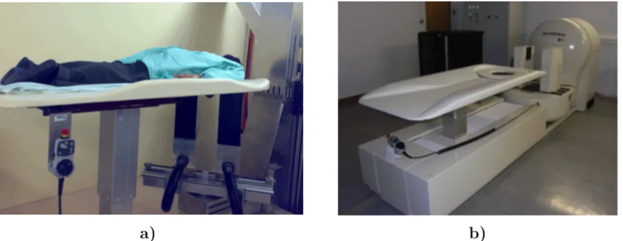
Figure 2.12 – Pictures of the PEM prototypes developed by the ConsortiumPET-Mammography: a) Clear-PEM prototype during an acquisition with a patient and b) Clear-PEM Sonic. Adapted from [80,81]. ... 28
!
Figure 2.13 – Scheme of the Clear-PEM detector heads (at centre). The acquisition geometry(at right) and the composition of one module (at left) are also shown. The PCBs (of Printed Circuit Board) that connect the APDs to the detector electronics are indicated. Adapted from [90,91]. ... 29
!
Figure 2.14 – Illustration of the detection geometry of the Clear-PEM scanner: a) a lesionlocated in a region between the detector heads produces a detectable LOR and b) a lesion located in a region above the detector heads do not produces a detectable LOR. ... 30
!
Figure 2.15 – Illustration showing a possible solution to enable chest wall imaging in theClear-PEM scanner. Two collimators, whose holes are oriented toward the chest, are coupled to the detector heads in order to allow the detection of lesions within the chest wall region. ... 30
!
Figure 3.1 – Illustration showing the breast in prone position and the basic half-ellipsoidalgeometry for the breast model. ... 38
!
Figure 3.2 – Illustration showing a possible solution to enable chest wall imaging in aconventional dual head SPEM system. The dashed lines show the collimator FOV. ... 39
!
Figure 3.3 – Illustration showing the parameters used in the selection criteria proposed byZeng. The dashed lines represent the field of view of the pinhole collimator. The parameter f is the focal distance required to image an object with axial dimension O and at object-focus distance b, with a detector size G. ... 41
!
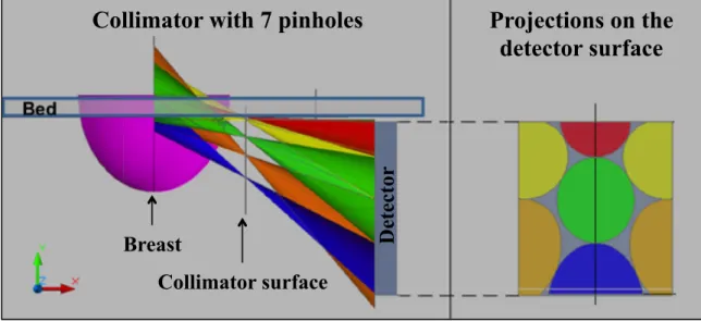
Figure 3.4 – Scheme of a collimator with 7 pinholes. The position of the pinholes (at left)and their projections at the detector surface (at right) are shown. ... 42
!
Figure 3.5 – Illustration showing: (a) Non-matched collimator design and (b) Matchedcollimator design. The useful active area of the detector is less than maximum, when the collimator septa (blue) differ in size or are not aligned with the pixels (gray). ... 43
!
Figure 3.6 – Schematic of the side view of a fan beam collimator (convergent in x direction and parallel in y direction). The collimator thickness L0, hole diameter d0 (at the
detector side), septal thickness t0, pixel pitch p0, source-collimator distance z0,
source-detector distance z0’, focal distance f and focus-detector distance f’, are
indicated. The black dashed lines at the centre of the holes represent the hole axis with different incidence angles β. ... 44
!
Figure 3.7 – Illustration showing the variation of local efficiency along the FOV. Thesensitivity is higher for regions located directly over the central collimator holes (incidence angle β=0). ... 46
!
Figure 3.8 – Illustration showing the minimum distance zmin beyond which a source S can bedetected in adjacent holes. A ray emitted from a source S at a distance zmin is
shown. The collimator thickness L0, focal distance f, the hole diameter d0, the
septal thickness t0 and the pixel pitch p0 are indicated. ... 48
!
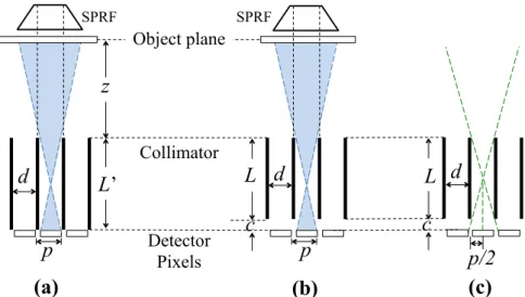
Figure 3.9 – Illustration showing: (a) the conventional matched collimator design to avoid multiplexing (parallel hole collimator); and (b) the design where multiplexing occurs, since photons arriving from different collimator holes can hit the same detector pixel. For each case the single pixel response function, SPRF (2D view), is shown. The collimator thickness L, object-collimator distance z, collimator-detector distance c, hole diameter d and pixel size p are indicated. ... 49
!
Figure 3.10 – Illustration showing the approach used to calculate the spatial resolution of theparallel hole collimator design with multiplexing. The continuous SPRF (green line) and real response function (black line) are shown. The object-collimator distance z, collimator thickness L, collimator-detector distance c, the hole diameter d and pixel pitch p, are indicated. ... 50
!
Figure 3.11 – Illustration showing the approach used to calculate the spatial resolution of thecone beam collimator design with multiplexing. The continuous SPRF (green line) and real response function (black line) are shown. The distance B is the width of the small triangle used in the calculation of the resolution. The object-collimator distance z0, collimator thickness L0, collimator-detector distance c, the hole
diameter d0 and pixel pitch p0, are indicated. ... 51
!
Figure 3.12 – Illustration showing: (a) a conventional matched collimator design, (b) a collimator design with a small collimator-detector distance c (where the multiplexing do not occur), and (c) the geometry used to calculate the criterion that determines if the multiplexing effect occurs. Note that the collimators in (a) and (b) have the same response function and, therefore, the same spatial resolution. ... 53
!
Figure 3.13 – Schematic of the convergent collimator. The hole at the left (incidence angle β)looks like a parallel hole with length L, septal thickness t and hole diameter d. The collimator thickness L0, focal distance f, the hole diameter d0, the septal thickness
t0 and the pixel pitch p0 are indicated. ... 55
!
Figure 3.14 – A flowchart representing the steps of the optimization algorithm. The algorithm determines the collimator dimensions (hole diameter dopt, collimator
thickness Lopt and focal distance fopt) that maximize the local sensitivity, for the
desired input parameters (incidence angle β, linear attenuation coefficient of the collimator material µ, source-collimator distance z0, pixel size p0, spatial resolution
Figure 3.15 – Optimized collimator dimensions (for tungsten, µ=34.48 cm-1 at 140 keV) as a
function of the hole incidence angle β: (a) the optimal hole diameter and (b) the optimal collimator thickness. ... 59
!
Figure 3.16 – Schematic of the Field Of View of a convergent collimator. The dimension O isthe object size or the FOV axial dimension required to image an object at a source-collimator distance z0. The focal distance f, the collimator thickness L0, and the
detector size G are indicated. ... 61
!
Figure 3.17 – Average sensitivity of optimal convergent collimators (tungsten, µ=34.48 cm-1at 140 keV) as a function of the focal distance f: (a) and (b) fan beam geometry, (c) and (d) cone beam geometry. The results were obtained for different values of spatial resolution (3.0 and 7.5 mm) and source-collimator distance (3.0-7.0 cm), considering a fixed pixel size p0=1.6 mm and detector size G=20 cm. ... 62
!
Figure 3.18 – Schematic of the parallel, fan and cone beam collimator designs. The dimension O is the object size or the FOV axial dimension required to image the object at a source-collimator distance z0. The focal distance f, the collimator thickness L0, and
the detector size G are indicated. ... 63
!
Figure 3.19 – Schematic of the collimator and FOV dimensions: (a) axial FOV dimensionsand (b) transverse FOV dimensions. The collimator thickness L0, object-collimator
distance z0, object-detector distance z0’ and focus-detector height H are indicated.
The focal distance f, focus-detector distance f’, detector size G and FOV size O are shown for both x and y directions. ... 67
!
Figure 3.20 – Schematic of the collimator and FOV dimensions: (a) axial FOV dimensionsand (b) transverse FOV dimensions. The collimator thickness L0, object-collimator
distance z0, object-detector distance z0’, collimator-detector distance c and
focus-detector height H are indicated. The focal distance f, focus-focus-detector distance f’, detector size G and FOV size O are shown for both x and y directions. ... 71
!
Figure 3.21 – Illustration showing the shielding provided by the detector heads. The redareas show the torso regions that are introduced in the collimator FOV and detected in the top of the detector. ... 74
!
Figure 4.1 – Front view of the detector model. The size of the crystals and the spacingbetween them are shown. ... 81
!
Figure 4.2 – Geometry of the model that was implemented in GATE to simulate the SPEMscanner with the projected collimator: (a) side view showing the detector axial dimension (b) top view showing the detector transverse dimension. The dimensions of the collimator, crystals and detector shielding are shown (in millimetres). A CAD software (Computer-Aided Design) was used to open and visualize the GATE geometry file. ... 82
!
Figure 4.3 – Schematic of the digitizer modules used in the simulation. The chain of modulesbegins with the hits and ends with the single. ... 83
!
Figure 4.4 – Front view of the Clear-PEM detector model. The supermodule, module, crystalsize and the gap dimensions are shown. ... 85
!
Figure 4.5 – Geometry of the model that was implemented in GATE to simulate theClear-PEM scanner with the projected collimator: (a) side view showing the detector axial dimension (b) top view showing the detector transverse dimension. The
dimensions of the collimator, crystals, detector shielding and other detector components are shown (in millimetres). ... 85
!
Figure 4.6 – (a) 176Lu decay scheme to 176Hf. In 99.66% of the cases, 176Lu decays into 176Hf bybeta-emission at 596.82 keV, followed by a cascade of gamma photons with energies of 307, 202 and 88 keV. (b) The full 176Lu background spectrum of single
events in the Clear-PEM scanner. The three peaks correspond to the gamma ray energies of 88, 202 and 307 keV. The highest energy in the background spectrum agrees with the total available energy in the decay process, Qβ-=1194 keV (Adapted
from [83]). ... 87
!
Figure 4.7 – Front view of the Derenzo phantom and scheme of the acquisition geometry(used in the simulation of both SPEM and Clear-PEM systems). The diameter of the rods and the distance between the axis of rotation and collimator surface are shown. ... 88
!
Figure 4.8 – Front view of the Defrise phantom and scheme of the acquisition geometry(used in the simulation of both SPEM and Clear-PEM systems). The cylinder and disk dimensions and the distance between the axis of rotation and collimator surface are shown. ... 89
!
Figure 4.9 – 3D views of the XCAT phantom voxelized geometry. The different organ andbone structures are shown. ... 90
!
Figure 4.10 – (a) Cranio-caudal view showing the XCAT phantom and the acquisitiongeometry that was implemented in GATE to simulate a real breast exam (b) Schematic showing the location and diameter of the simulated breast lesions. ... 91
!
Figure 4.11 – Front view of the acquisition geometry that was implemented in GATE tosimulate the response functions of the following systems: (a) SPEM system (b) Clear-PEM system. In both images the detector head (gray), collimator (blue) and cylindrical source (yellow) are shown. ... 98
!
Figure 4.12 – SPEM system resolution as a function of distance from collimator surface. Thesimulated resolution values, including the one at the centre of the FOV (FWHMz=5cm), and the line representing the theoretical resolution are shown. ... 98
!
Figure 4.13 – Clear-PEM system resolution as a function of distance from collimator surface. The simulated resolution values, including the one at the centre of the FOV (FWHMz=5cm), and the line representing the theoretical resolution are shown. ... 99
!
Figure 5.1 – Illustration of the discretized 2D image and projection. The pixel value fj, the
projection bin pi and the weighting factor aij are indicated. ... 104
!
Figure 5.2 – Illustration of the methods used to calculate the system matrix: (a) the ray-driven method and (b) Monte Carlo simulation method. ... 106
!
Figure 5.3 – Illustration showing face-to-face detector heads, with parallel beam collimators,measuring the same projection ray. ... 107
!
Figure 5.4 – Schematic of the different scanning trajectories of the cone beam focal point: (a)Circular orbit, (b) Helical orbit and (c) Circle-and-line orbit. Tuy’s condition is analysed on each case. ... 108
!
Figure 5.5 – Defrise phantom reconstructed from: (a) complete projection data and (b)blurring artefacts are more prominent in the bottom disks of the phantom, located away from the orbit plane (defined by the cone beam focal point). ... 108
!
Figure 5.6 – Reconstructed image of the Derenzo phantom acquired with SPEM scanner(central transverse slice, 40th MLEM iteration). The plot on the right shows the
profile taken along the line indicated on the image. ... 111
!
Figure 5.7 –Reconstructed image of the Defrise phantom acquired with SPEM scanner(central transverse slice, 40th MLEM iteration). The plot on the right shows the
profiles taken along two lines with 3 cm spacing between them. The green line crosses the centre of the phantom. The line profiles were used to measure the image distortion, ∆x, along the first disk of the phantom. ... 111
!
Figure 5.8 – Reconstructed images of the XCAT breast phantom obtained from the SPEMsimulated data (simulated acquisition time of 11 minutes, lesion to breast ratio of 6:1). The reconstructed images correspond to the central transverse plane (cranio-caudal view) and were obtained for different MLEM iterations: (a) 10 iterations; (b) 20 iterations; (c) 30 iterations and (d) 40 iterations. ... 112
!
Figure 5.9 – Reconstructed images of the XCAT breast phantom obtained from the SPEMsimulated data (simulated acquisition time of 21 minutes, lesion to breast ratio of 6:1). The reconstructed images correspond to the central transverse plane (cranio-caudal view) and were obtained for different MLEM iterations: (a) 10 iterations; (b) 20 iterations; (c) 30 iterations and (d) 40 iterations ... 113
!
Figure 5.10 – XCAT breast image analysis: (a) Regions of interest used to perform theanalysis of the reconstructed images; (b) and (c) plots of the lesion contrasts and signal-to-noise ratios against iteration number, respectively. ... 114
!
Figure 5.11 – Selected image estimates of the XCAT breast phantom with the chest wall (3mm) and breast (6 mm) lesions, located at 4 and 3 cm in the position axis, respectively. The images at the left show the central transverse planes (cranio-caudal view) acquired with different acquisition times: (a) 11 minutes and (b) 21 minutes. The plots at the right show the profiles taken over a line that crosses the centre of the chest wall (green) and breast lesions (blue). ... 115
!
Figure 5.12 – Reconstructed image of the Derenzo phantom acquired using the Clear-PEMscanner with the projected collimator (central transverse slice, 40th MLEM
iteration). The plot on the right shows the profile taken along the line indicated on the image. ... 116
!
Figure 5.13 – Reconstructed images of the Defrise phantom acquired with the Clear-PEMscanner with the projected collimator (central transverse slice, 40th MLEM
iteration). The plot on the right shows the profiles taken along two lines with 3 cm spacing between them. The green line crosses the centre of the phantom. The line profiles were used to measure the image distortion, ∆x, along the first disk of the phantom. ... 116
!
Figure 5.14 – Reconstructed images of the XCAT breast phantom obtained from theClear-PEM simulated data (simulated acquisition time of 11 minutes, lesion to breast ratio of 6:1). The reconstructed images correspond to the central transverse plane (cranio-caudal view) and were obtained for different MLEM iterations: (a) 10 iterations; (b) 20 iterations; (c) 30 iterations and (d) 40 iterations. ... 117
!
Figure 5.15 – Reconstructed images of the XCAT breast phantom obtained from the Clear-PEM simulated data (simulated acquisition time of 21 minutes, lesion to breast ratio of 6:1). The reconstructed images correspond to the central transverse plane (cranio-caudal view) and were obtained for different MLEM iterations: (a) 10 iterations; (b) 20 iterations; (c) 30 iterations and (d) 40 iterations. ... 118
!
Figure 5.16 – Breast image analysis: (a) Regions of interest used to perform the analysis ofthe XCAT breast phantom reconstructed images; (b) and (c) plots of the lesion contrasts and signal-to-noise ratios against iteration number, respectively. ... 119
!
Figure 5.17 – Central transverse plane (cranio-caudal view) of the reconstructed images ofthe XCAT breast phantom with the chest wall (3 mm) and breast (6 mm) lesions. The plot at the right shows the profiles taken over a line that crosses the centre of the chest wall (blue) and breast lesions (green). ... 119
!
Table 2.1 – Summary of the commercial SPEM scanners specifications. The main specifications of each system are presented (PSPMT: position sensitive photomultiplier tube; NaI: sodium iodide; CZT: cadmium zinc telluride). ... 22
!
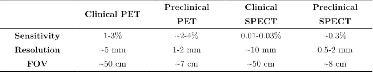
Table 2.2 – Main performance characteristics of clinical and preclinical SPECT and PETscanners. Adapted from [15]. ... 26
!
Table 2.3 – Summary of the commercial PEM scanners specifications. The mainspecifications of each system are presented (LYSO: lutetium yttrium oxyorthosilicate; PSPMT: position sensitive photomultiplier tube; FOV: field of view; DOI: depth-of-interaction). ... 28
!
Table 3.1 – The selected values for the half-ellipsoidal dimensions and the breast axes alongwhich they are measured. ... 38
!
Table 3.2 - Optimal collimator dimensions for low energy radiation (140 keV), calculatedusing the optimization algorithm for different input parameters (O=10 cm, G=20 cm, z0=5 cm, µ=34.48 cm-1) and geometries [PB=Parallel Beam, FB=Fan Beam
and CB=Cone Beam]. ... 64
!
Table 3.3 - Optimal collimator dimensions (collimator thickness L0, hole diameter d0, septalthickness t0, focal distance f and zmin value) for different input spatial resolutions.
The collimator weight and average sensitivity are also shown. ... 68
!
Table 3.4 - Optimal collimator dimensions (collimator thickness L0, hole diameter d0, septalthickness t0, focal distance f and zmin value) after introducing the manufacturing
limitations. ... 69
!
Table 3.5 – Final collimator dimensions (collimator thickness L0, hole diameter d0, septalthickness t0, focal distance f and zmin value) and specifications (resolution, average
sensitivity and βx min) for the dual-head SPEM scanner. ... 70
!
Table 3.6 - Optimal collimator dimensions (collimator thickness L0, hole diameter d0, septal
thickness t0, focal distance f and zmin value) for different input spatial resolutions.
The collimator weight and average sensitivity are also shown. ... 72
!
Table 3.7 – Final collimator dimensions (collimator thickness L0, hole diameter d0, septalthickness t0, lattice unit size p’, focal distance f and zmin value) and specifications
(resolution, βx min, weight and average sensitivity) for the Clear-PEM scanner. ... 73
!
Table 4.1 – List of parameters used to generate the female patient model from the XCAT phantom. ... 90
!
Table 4.2 – The elemental compositions and densities of the biological tissues used in theTable 4.3 – The Tc-99m-sestamibi concentrations (activity per unit volume) and corresponding radioactive ratio relative to breast for the various organs and lesions of the XCAT phantom. ... 93
!
Table 4.4 – The simulation results of the SPEM scanner with the projected collimator. Theacquisition times are shown in parentheses after the phantom name. ... 94
!
Table 4.5 – The simulation results of the Clear-PEM scanner with the projected collimator.The acquisition times are shown in parentheses after the phantom name. ... 95
!
Table 4.6 – The average count rates per crystal measured in the Clear-PEM imaging studies.The count rates from the LYSO:Ce background and phantom activities are shown. ... 95
!
Table 4.7 – Average sensitivity of the SPEM scanner, simulated using only one detector headwith the optimal collimator. ... 99
!
Table 4.8 – Average sensitivity of the Clear-PEM scanner, simulated using only one detectorhead with the optimal collimator. ... 100
!
Table 5.1 – Quality parameters of the XCAT phantom images, obtained from the SPEMsimulated data. The contrast, signal-to-noise ratio (SNR) and contrast recovery coefficient (CRC) values are shown for both selected image estimates, acquired during: 11 and 21 minutes. ... 115
!
Table 5.2 – Quality parameters of the XCAT phantom images, obtained from theClear-PEM simulated data. The contrast, signal-to-noise ratio (SNR) and contrast recovery coefficient (CRC) values are shown for the selected image estimate, acquired during 21 minutes. ... 120
!
Single Photon Emission Mammography with Convergent Collimators xxvi 18FDG 18F-fluorodeoxyglucose
2D two-dimensional
3D three-dimensional
APD Avalanche Photo-Diodes
BCT Breast Computed Tomography
BSGI Breast Specific Gamma Imaging
CERN European Organization for Nuclear Research
CRC Contrast Recovery Coefficient
CT Computed Tomography
CZT CdZnTe (cadmium zinc telluride)
DBT Digital Breast Tomosynthesis
DOI Depth Of Interaction
FOV Field Of View
FWHM Full Width at Half Maximum
GATE Geant4 Application for Tomographic Emission
GPS General Particle Source
ICRU International Commission on Radiation Units and measurements
LOR Line Of Response
LSO Lutetium Oxyorthosilicate
LYSO Lutetium Yttrium Oxyorthosilicate
MBI Molecular Breast Imaging
MLEM Maximum-Likelihood Expectation-Maximization
MRI Magnetic Resonance imaging
NCAT NURBS-based Cardiac-Torso (known as XCAT) NURBS Non-Uniform Rational B-Splines
OSEM Ordered-Subset Expectation-Maximization
PCB Printed Circuit Board
PEM Positron Emission Mammography
PET Positron Emission Tomography
PMT Photomultiplier Tube
PSRF Point Source Response Function
ROI Region Of Interest
SNR Signal-Noise-Ration
SNR Signal to Noise Ratio
SPECT Single Photon Emission Computed Tomography SPEM Single Photon Emission Mammography
SPRF Single Pixel Response Function
Part I:
C H A P T E R
1
1
Introduction
Breast cancer is the most frequent malign neoplasm and one of the leading causes of death by cancer among women worldwide [1]. Early diagnosis remains the best method of improving the survival rates of the patients. In this context, last years have witnessed the development of medical imaging techniques that have been important tools for the detection, diagnosis and clinical management of cancer, among other applications [2].
X-ray mammography is currently the most widely method used for breast cancer imaging and it is the only modality demonstrated to decrease the breast cancer mortality when used in regular screening programs [3]. However, the information provided by this technique is mainly anatomical and the exam sensitivity is reduced, particularly when imaging dense breast tissue in young women [4]. Due to these limitations, accurate second-line methods are needed in some instances to provide further information about suspicious lesions and to reduce the number of unnecessary invasive procedures, such as biopsies.
The radionuclide based imaging techniques, namely the positron emission tomography (PET) and the single photon emission computed tomography (SPECT), offer substantial potential as complementary diagnostic tools. These imaging techniques can provide an accurate assessment of the presence and extent of disease as well as unique information about tumour biological characteristics (rate of proliferation and metabolic activity) [5]. However, the general SPECT and PET systems were not designed for breast imaging applications. Therefore dedicated compact cameras for breast cancer imaging, such as single photon emission mammography (SPEM) and positron emission mammography (PEM) systems, have been intensively investigated over the past decade and can provide better sensitivity and spatial resolution than general systems [6].
The Clear-PEM scanner is a PEM system that was developed by a Portuguese research consortium and is able to detect, with high resolution and sensitivity, small cancerous lesions (approx. 2 mm) in the breast at an early stage of the disease [7]. The scanner is composed by two opposite detector heads that are placed near the breast (with the patient in prone position), allowing the detection of the uptake of a positron emitter radiotracer that was previously administered to the patient. However, given this detection geometry, it is only possible to detect coincidences in which the positron annihilation occurred in a region between the detector heads. In fact, the pairs of photons emitted (after the positron annihilation, with an angle of approximately 180° between them) from positions outside this region do not produce a detectable line of response (LOR). Therefore, the lesions located above the detector heads are not detected. These regions include the chest wall and axillary regions, which are important areas for cancer diagnosis [5]. The limitation in detecting lesions above the detector heads results in viewing a truncated breast volume in the image. This limitation is not exclusive to the Clear-PEM system; it is also an issue, in general, to conventional SPEM systems that use parallel hole collimators and orient the detector surface parallel to the breast’s central axis (nipple to chest direction) [8]. For this reason, several studies have been carried out in order to overcome this imaging limitation [9-14].
In this work, we investigate simpler and more efficient solution to solve the SPEM imaging limitation in detecting lesions in the chest wall region. In fact, by using an appropriate collimation geometry in which the field of view (FOV) includes the entire breast volume and chest wall, it is possible do detect lesions in regions not detected by the conventional collimators. Since this research was performed within the framework of the Clear-PEM project, it is also intended to research the feasibility of using the Clear-PEM system to image the chest wall region. With the acquisition in singles mode (or SPECT mode) and by adapting the same collimation geometry developed for the SPEM systems, it should be possible to image the chest wall region; something that is not possible using the system in PET mode. In both SPEM and Clear-PEM scenarios, the projected collimator should allow detecting lesions with high spatial resolution (2-3 mm) and sensitivity values (0.01-0.03 %) comparable to those of clinical SPECT systems [15]. The additional information obtained with the final solution could contribute for a better diagnosis of breast cancer.
Different collimation geometries are analysed in this work, with the aim of finding the best collimator to image the entire breast and adjacent regions. The proposed collimators are projected and simulated for two different systems: a SPEM scanner and the Clear-PEM scanner (in singles mode). These simulated data are used to study the feasibility of the solutions and to compare the results obtained for both scenarios. The simulated data is also used to assess dedicated SPECT image reconstruction algorithm, which was also developed and investigated in the context of this study.
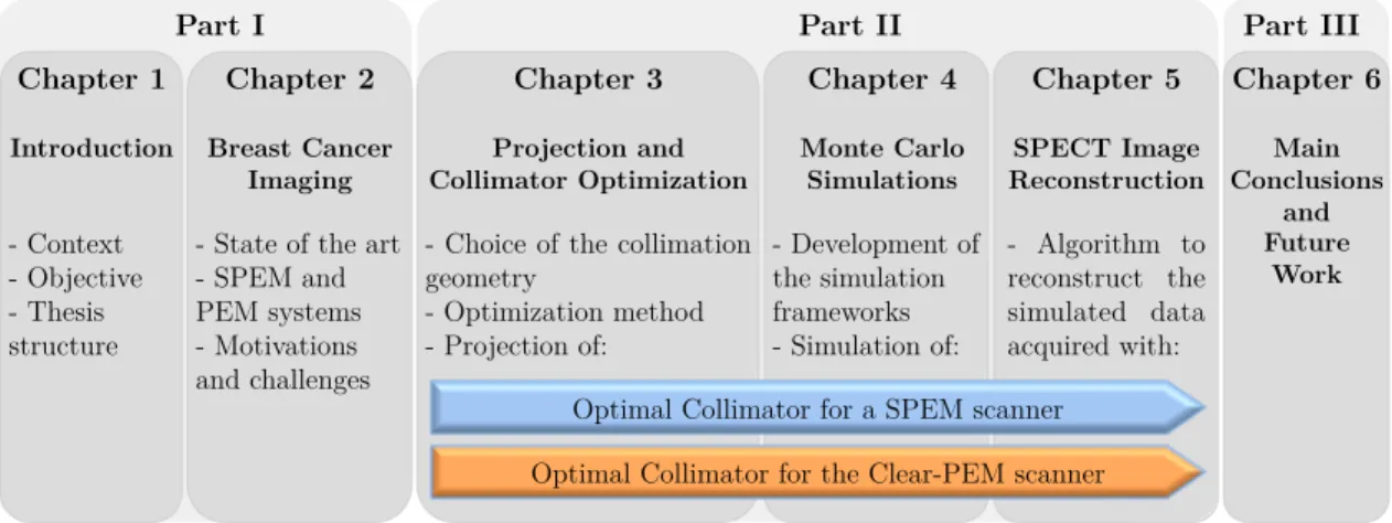
This thesis is divided into six chapters, in which each one addresses a specific task/part of this PhD work. The chapters are organized in three parts.
The Part I – Introduction and Background is composed by the present Chapter 1 – Introduction, where the context, objective, motivations and general organization of the work are provided; and by the Chapter 2 – Breast Cancer Imaging, which includes a review of the state of the art and the main knowledge fields that are related to the work presented in this thesis. An introduction to the breast cancer imaging techniques is provided with special focus on the Nuclear Medicine techniques, namely PET and SPECT. The physical principles and properties of these radionuclide based imaging systems, including both SPEM and PEM systems, are also described. A brief description of the SPEM systems that permit to image the entire breast volume (chest wall included) is provided. Finally, the Clear-PEM scanner specifications are presented, as well as the motivations and challenges involved in adapting this system for SPECT acquisitions.
The Part II – Methods and Results comprises three chapters that describe the methods handled to achieve the objective of this work and present the results obtained for the proposed solutions. The Chapter 3 – Projection and Collimator Optimization is devoted to the study and selection of the appropriate collimation geometry to image the breast and chest wall region. An optimization algorithm for converging collimators, developed in this work, is also described. Optimal cone beam collimators are calculated and projected in order to adapt to the SPEM system and the Clear-PEM prototype characteristics. The performances of the optimal collimators obtained for the Clear-PEM scanner are compared to those obtained for a SPEM system with the same detector size and collimation geometry. The following chapter, Chapter 4 – Simulation, describes the Monte Carlo simulations of the proposed imaging setting and the main results obtained. The simulation framework that was developed to study both systems expected performance (with the collimators optimized in the previous chapter) is presented. This chapter also includes a description of the settings and the phantoms used in the simulations. The final chapter of Part II is Chapter 5 – SPECT Imaging Reconstruction, which describes the reconstruction algorithm developed to reconstruct the simulated data acquired with the proposed collimators. The results obtained for different simulated scenarios are compared and analysed. An overall discussion of the results and on the feasibility of the proposed image setting is provided at the end of this chapter.
The Part III – General Conclusion is the last section of this document, which is compounded by the Chapter 6 – Main Conclusions and Future Work. In this chapter, a global discussion of the results and main findings of this work are presented, together with our perspectives for future work.
The diagram in Figure 1.1 shows the thesis structure and the main topics addressed in each part.
At the end of this document, the appendix section lists all publications and conference proceedings in which part of the work presented in this thesis was published.
Figure 1.1 – Diagram showing the thesis structure and the main topics.
Chapter 2
Breast Cancer Imaging
- State of the art - SPEM and PEM systems - Motivations and challenges Chapter 3 Projection and Collimator Optimization
- Choice of the collimation geometry - Optimization method - Projection of: Chapter 4 Monte Carlo Simulations - Development of the simulation frameworks - Simulation of: Chapter 5 SPECT Image Reconstruction - Algorithm to reconstruct the simulated data acquired with: Optimal Collimator for a SPEM scanner
Optimal Collimator for the Clear-PEM scanner
Chapter 6 Main Conclusions and Future Work
Part I Part II Part III
Chapter 1 Introduction - Context - Objective - Thesis structure
C H A P T E R
2
2
Breast Cancer Imaging
2.1 Introduction
Breast cancer is the most common type of cancer affecting a growing number of women worldwide. The incidence rates of breast cancer increased from 641,000 cases in 1980 to 1,643,000 cases in 2010, which correspond to an annual increase rate of 3.1 %. The global breast cancer mortality rate is also high. In 2010 were registered 425,000 victims, of whom 68,000 were aged 15-49 years in developing countries [16].
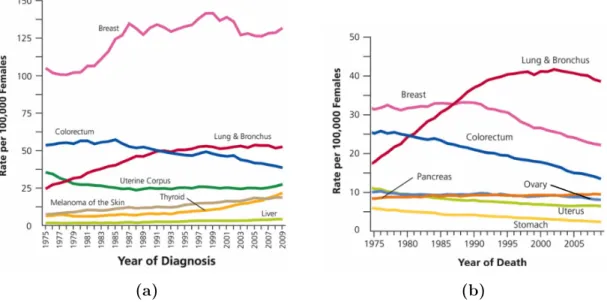
According to the American Cancer Society, breast cancer has the highest incidence rate (Figure 2.1(a)) and is the second leading cause of cancer death among women in the United States (Figure 2.1(b)), second only to lung cancer [1]. Figure 2.1(a)
(a) (b)
Figure 2.1 – Incidence rates and death rates among females for selected cancers, United States, 1975 to 2009: (a) Incidence rates and (b) Death rates (Uterus includes uterine cervix and uterine corpus). Adapted from [17].
shows an increase of the incidence rates for female breast cancer during the 1980’s. This increase is related to the growth of the screening programs that allowed a higher number of breast cancer diagnosis [18]. The decrease in death rates for female breast cancer, shown in Figure 2.1(b), is due to the improvements in early detection and/or treatment [17].
The most frequent type of breast cancer is the ductal carcinoma, which begins in cells that line a breast duct (see Figure 2.2), and the second most common is the lobular carcinoma, which begins in a lobule of the breast [19]. Both ductal and lobular carcinoma can degenerate into invasive carcinoma if the cancer spreads to surrounding breast tissues. Since the first sites to receive the lymph from the tumour cells are the axillary lymph nodes, the sentinel lymph node biopsy is usually performed to ascertain if the tumour has spread to other regions of the body (metastasis) [20].
Figure 2.2 – Illustration showing the anatomy of the female breast. The nipple and the areola are shown on the outside of the breast. The axillary lymph nodes network, ducts, lobules and other parts of the inside of the breast are also shown (Adapted from [19]).
The breast imaging techniques play an important role in the detection, diagnosis and clinical management of breast cancer. The most common used imaging modalities include X-ray mammography, magnetic resonance imaging (MRI), ultra-sonography (US) and radionuclide imaging, such as single photon emission computed tomography (SPECT) and positron emission tomography (PET) [2]. In this chapter we will overview the physical principles inherent to each of these breast modalities, as well as the main advantages, pitfalls and the characteristics of the information they can provide about the body tissues. A reference to the recent technological advances and alternative breast imaging approaches will be provided. Given the context of this work, a special focus will be done to the breast-specific radionuclide imaging systems.
2.1.1 X-ray mammography
X-ray mammography is essentially the only widely used method for breast cancer screening, which emerged as a screening tool after the mid-1960s [2]. The combination of mammography screening with improved treatment has shown to decrease the breast cancer mortality rates [3]. This imaging technique relies on differences in the attenuation of low energy x-rays to distinguish cancer from healthy breast tissues. However, these differences are mainly observable in areas of fatty breast tissue. In areas of dense breast tissue, the density differences between cancerous lesions and surrounding healthy tissues is low [21]. As a result the tumours can be overlapped and, therefore, undetectable in the mammogram. Hence, the exam sensitivity1 for the detection of small
breast lesions is reduced in women with dense breast tissue. While the overall sensitivity of mammography has been reported as ranging from 77% to 95% [3], in women with mammographically dense breasts the sensitivity value ranges between 48% and 63% [22]. This limitation is particularly important due to the fact that dense breast tissue is also a risk factor for breast cancer [4]. Besides the specificity2 of mammography has been
recently reported as ranging from 94% to 97% [3], false positive results are common (specially in dense breast) and can cause anxiety and lead to additional imaging studies or invasive procedures (such as biopsy or fine-needle aspiration). Therefore, given this low ability to distinguish cancerous from noncancerous lesions and the high number of inconclusive screened cases, a breast lesion evaluation based uniquely on x-ray mammography results frequently in unnecessary biopsies or additional exams, which are financially expensive to health institutions [3].
Due to the x-ray mammography limitations, new clinical applications that involve the use of contrast agents are being developed in order to map the distribution of neovasculature induced by cancer using mammography [23]. Also, other modalities have been proposed as additional adjunct diagnostic methods for improving the breast cancer detection and diagnosis, as described bellow.
2.1.2 Magnetic Resonance Imaging
Magnetic resonance imaging (MRI) has an important role in breast imaging as an adjunctive tool for screening and as a diagnostic tool for imaging lesions that are indeterminate from other modalities [2]. MRI is an imaging technique that makes use of the property of nuclear magnetic resonance to obtain detailed images of the hydrogen
1 Sensitivity is the number of true positives divided by the sum of true positives with
false negatives (negative diagnosis that were lately proved to be false).
2 Specificity is the number of true negatives (negative diagnosis that were lately
nuclei density inside the human body. The MRI scanners have a powerful magnet where the magnetic field is used to align the magnetization of the hydrogen nuclei and a coil that produces radio frequency pulses to systematically induce a modification in this alignment. As a result the nuclei produce a rotating magnetic field that is detected by the scanner and recorded to construct the image. Since the tissues have different hydrogen nuclei densities, MRI can create more detailed images of the human body than those obtained with x-rays [24]. Additionally, MRI has the advantage of not using ionizing radiation.
The first in vivo breast MRI studies were reported in the early 80’s. Since then, the technological improvements and the development of novel image acquisition techniques expanded its clinical applications [24]. Recent clinical studies, in women with high-risk of breast cancer, demonstrated the MRI ability to detect mammographically occult cancers with higher sensitivity than x-ray mammography [25] but with low specificity [25,26]. Besides the low specificity, MRI has three other handicaps: the high cost of the exam, the limited access and the difficulty in performing a guided biopsy (it is time consuming and requires the use of MRI compatible needles) [27]. Additionally, the dynamic contrast enhanced breast MRI, which is an image acquisition technique clinically used to provide volumetric three-dimensional (3D) anatomical and physiologic information of the breast, requires the injection of a contrast agent that entails some elevated risk to the patient [2].
2.1.3 Ultrasound imaging
Breast ultra-sound or ultra-sonography (US) is an imaging technique that plays a critical role in the diagnostic evaluation of screening detected or palpable breast masses [28]. US imaging involves the use of high frequency sound waves (a centre frequency above 10 MHz is the value recommended for breast US [29]) that are produced by a transducer and emitted through the region in study. Since the body tissues have different acoustic impedances, the US waves interact with the tissues producing different echoes that are detected outside the body and used to generate an image. Therefore, unlike x-ray imaging, US has the advantage of not using ionising radiation.
Breast US is a low cost imaging technique and essential for accurate non-invasive diagnosis of breast cysts. Since cystic masses are more fluid than tumours, they have different acoustic properties. In addition, breast US is also used in the examination of young or pregnant symptomatic patients, guidance of percutaneous needle interventions and in screening of some asymptomatic patients [28].
The results of a clinical study, which included 11,130 asymptomatic women, demonstrated that breast US has improved sensitivity (97%) when adjunctively used with x-ray mammography compared to physical examination and mammography
together (74%). Furthermore, it was also observed an improvement in sensitivity for dense breasts with US compared to mammography [30].
Some acquisition modes of breast US are already used to study the lesion vascularization. However the most common form of US imaging (B-mode US) produces noisy images containing artefacts [31]. Moreover, it is highly user dependent and the interpretation of the breast sonograms varies for different observers [28].
2.1.4 Radionuclide imaging
The radionuclide based imaging techniques, namely the positron emission tomography (PET) and the single photon emission computed tomography (SPECT), allow to explore the functional differences between normal and cancerous cells, which result from the different levels of radiotracer uptake. Since the radiotracer uptake is higher in cells with high metabolic rate (characteristic of cancer cells), these imaging techniques can provide an accurate assessment of the presence and extent of disease. In addition, one can obtain unique information about tumour biological characteristics, such as rate of proliferation and metabolic activity [5].
Given the unique information provided by these techniques (Figure 2.3), the sensitivity (above 90%) and specificity (up to 91%) for cancer identification are frequently higher in nuclear emission imaging than in other radiology modalities [32]. The functional information also complements the anatomical information provided by the conventional imaging techniques, such as x-ray imaging and ultrasound. Therefore, PET and SPECT offer substantial potential as complementary diagnostic tools [6] and also play an important role in the detection and localization of cancer cells that acquired the ability to spread to other organs or tissues in the body (metastasis) [5].
The majority of radionuclide imaging systems has detector geometries and specifications that are not appropriate for imaging small organs, which complicates its
Figure 2.3 - Diagram showing the information provided by each medical imaging modality based on its widespread use. Note that based on the widespread use of the breast imaging modalities both x-ray mammography and breast US provide mainly anatomical information, however it was considered their ability to provide functional information about the breast tissues.
Anatomic Functional/Physiologic Metabolic Molecular
X-ray imaging
MR imaging
Radionuclide imaging
US imaging
incorporation into standard practice for breast cancer imaging due to several reasons [33]: i) inadequate imaging geometry limits the proximity to the organ, which
results in poor detection sensitivity and low spatial resolution;
ii) the conventional cameras have low spatial resolution and signal-to-noise ration (SNR), inappropriate to detect small breast lesions;
iii) Relatively high cost and long scan times.
Thus, the potential importance of the application-specific, dedicated compact cameras for breast cancer imaging is clear. There have been many recent radioisotope imager developments for breast imaging, which are designated as single photon emission mammography (SPEM) or positron emission mammography (PEM) systems [6] (as we will see in the next sections: 2.2 and 2.3, respectively).
2.1.5 Other imaging modalities
It is important to mention that intense efforts are currently under way to improve the technological aspects of the aforementioned modalities and to develop new breast imaging techniques (the article by Karellas et al. [2] provides a complete overview).
Since the x-ray mammography reduces the three-dimensional (3D) anatomy of the breast into a two-dimensional (2D) image, the breast structures are overlapped creating a visually distracting mask that can mimic or obscure the presence of lesions. Therefore, 3D modalities, such as digital breast tomosynthesis (DBT) [34] and breast computed tomography (BCT) [35], are being actively investigated in order to provide depth information in x-ray mammography. However, these modalities need to show improved lesion detection with exam doses comparable to those used in mammography in order to be used as clinical tools for screening.
Optical imaging (uses light in the near infrared) [36] and microwave imaging (uses microwave frequency) [37] are alternative modalities that use different electromagnetic frequencies to image the optical and the dielectric properties of the tissues, respectively. These and other modalities are being investigated as alternative breast imaging approaches [38].
In addition to the improvements in each modality, the development of multimodality systems that combine the strengths of each modality is likely to become more widespread [6]. Finally, we are also likely to observe a change in the manner in which breast cancer screening will be performed in the future: the current standard manner (where mammography is the golden standard modality) is likely to be replaced by a personalised screening program where the selection of the imaging modalities would depend on several patient factors (such as the individual’s risk or breast density) [2].