The Mann-Kendall test: the need to consider the interaction between serial correlation and trend

(1)

http://www.uem.br/acta ISSN printed: 1679-9275 ISSN on-line: 1807-8621

Doi: 10.4025/actasciagron.v35i4.16006

The Mann-Kendall test: the need to consider the interaction between

serial correlation and trend

Gabriel Constantino Blain

Centro de Ecofisiologia e Biofísica, Instituto Agronômico, Cx. Postal 28, 13012-970, Campinas, São Paulo, Brazil. E-mail: gabriel@iac.sp.gov.br

ABSTRACT. Pre-whitening approaches have been widely used to remove the influence of serial correlations on the Mann-Kendall trend test (MK_prew). However, previous studies indicate that this procedure may lead to a false reduction of the significance of a trend. An alternative approach (MK_interact) has been proposed to improve the assessment of the significance of a trend in auto-correlated data. Therefore, the present study compared the performance of the MK_prew and MK_interact for detecting trends in auto-correlated series. Sets of Monte Carlo experiments were carried out to evaluate the occurrence of type I and II errors obtained from both approaches. The analyses were also based on 10-day values of the difference between precipitation and potential evapotranspiration (P-EP) obtained from the location of Campinas, State of São Paulo, Brazil. The results found in this study allow us to conclude that the MK_interac outperformed the MK_prew in correctly identifying the significance of trends and that, concerning agricultural interests, the decreasing trend described by the MK_interac during the beginning of the crop growing seasons may reveal an unfavorable temporal distribution of the P-EP values.

Keywords: Monte Carlo experiments, auto-correlated series, climate change, Pre-whitening.

Teste de Mann-Kendall: a necessidade de considerar a interação entre correlação serial e

tendência

RESUMO. O procedimento denominado pre-whitening vêem sendo largamente utilizado para remover a influência da correlação serial sobre o teste de tendência de Mann-Kendall (MK_prew). Entretanto, estudos anteriores indicam que essa abordagem pode resultar na redução errônea da significância de uma tendência. A fim de evitar esse possível erro, propôs-se o uso de um método alternativo (MK_interact) para melhorar a avaliação da significância desta última componente. Assim, o presente estudo comparou o desempenho do MK_prew ao do MK_interact na realização da referida análise. As probabilidades de ocorrência dos erros tipos I e II, obtidas a partir de ambos os procedimentos, foram avaliadas com base em experimentos de Monte Carlo. Utilizaram-se também séries decendiais da diferença entre a precipitação e a evapotranspiração potencial (P-ETP) da localidade de Campinas, Estado de São Paulo, Brasil. Os resultados permitem concluir que o MK_interac superou o MK_prew na correta identificaçãoda significância das tendências e, sob os interesses agrícolas, a tendência decrescente descrita pelo MK_interac durante o início do ano agrícola pode revelar uma distribuição temporal desfavorável dos valores de P-ETP.

Palavras-chave: simulações deMonte Carlo, séries auto-correlacionadas, mudanças climáticas, Pre-whitening.

Introduction

The nonparametric Mann-Kendall test (MK), also known as Kendall’s τau test or the Mann-Kendall trend test (KENDALL; STUART, 1967; MANN, 1945), is widely used to evaluate trends in agro-meteorological and hydrological time series (BLAIN, 2010; BLAIN, 2011a, b and c; BLAIN; PIRES, 2011; BURN; ELNUR, 2002; BURN et al., 2004; MINUZZI et al., 2011; SANSIGOLO, 2008; SANSIGOLO; KAYANO, 2010; STRECK et al., 2011; YUE et al., 2002 and 2003). As a consequence of this widespread use, several scientific studies have

addressed the strengths and the limitations of this statistical test. The strengths of the MK are usually associated with its simple concept and with the fact that as a nonparametric procedure that does not assume a specific joint distribution of the data, it is minimally affected by departures from normality (YUE; PILON, 2004).

(2)

Nevertheless, in practical applications, the rejection of such H0 is frequently taken as an evidence of the presence of a trend in a given (agro-meteorological and/or hydrological) time series. After Chandler and Scott (2011), we may assume that this last assumption is quite reasonable, as in iid datasets, (clearly) no trend is present.

However, as described in Von Storch and Navarra (1995), Yue et al. (2002), Burn and Elnur (2002), Burn et al. (2004), Sansigolo and Kayano (2010), Blain (2011a, b and c); Blain and Pires (2011), the presence of a significant positive serial correlation increases the number of false rejections of H0. In other words, the presence of such a component increases the occurrence of type I errors, making it greater than the (adopted) nominal significance level.

Based on Monte Carlo simulations, Yue et al. (2002) demonstrated that the number of rejections of true H0 increases as the positive serial correlation increases. According to Yue et al. (2002), these results concur with the results obtained by Von Storch and Navarra (1995). Therefore, in practical applications, a significant MK result can arise either due to the presence of a genuine trend or because the data are auto-correlated (CHANDLER; SCOTT, 2011). Although this feature is important in any trend analysis, it is of particular interest for agro-meteorological studies, which frequently exhibit positive auto-correlation coefficients (WILKS, 2006; BLAIN; PIRES, 2011). However, by following Sansigolo and Kayano (2010), we may indicate that the aforementioned feature is nonetheless neglected in Brazilian agro-meteorological studies. Thus, efforts to ensure that the aforementioned H0 will be correctly rejected are of great interest.

Authors such as Von Storch and Navarra (1995), Zhang et al. (2000), Burn and Elnur (2002), Blain (2011b); Blain and Pires (2011), among many others, have proposed or used pre-whitening approaches to remove the effect of serial correlations on the aforementioned trend test. However, according to Yue et al. (2002 and 2003) and Burn et al. (2004), although this widely used approach was developed to limit the influence of autocorrelations on the MK results, it does not address the potential interaction between this last component and an existing trend. As indicated in the significant study of Yue et al. (2002), the removal of a positive auto-correlation component by pre-whitening a given dataset may result in an erroneous reduction of the significance of an existing trend. Moreover, estimating the auto-correlation coefficients prior to

the removal of the trend may lead to overestimating such coefficients. To overcome these difficulties, Yue et al. (2002) developed an alternative algorithm (referred to as the trend free pre-whitening approach; MK_interac) that is capable of dealing with this interaction between trend and autocorrelation. According to these authors, the MK_interac provides a correct estimate of the significance of an existing trend. Furthermore, Yue et al. (2002) also states that with the MK_prew, ‘researches and practitioners may have incorrectly identified the possibility of significant trend’.

This last statement, associated with the assumption that the correct assessment of the significance of a given climate trend is an essential step in dealing with climate change implications, reinforces the need to compare the performance of the two approaches (MK_interac and MK_prew) for detecting trends in the presence of serial correlation. Thus, for this purpose, we first carried out sets of Monte Carlo experiments to evaluate both the type I and the type II errors obtained from the MK_interac

and MK_prew. As a second step, we applied both MK approaches to 10-day values of the difference between precipitation and potential evapotranspiration (P-EP) obtained from the weather station of Campinas, State of São Paulo, Brazil. It is expected that this study should provide a deeper understanding of the MK_interac calculation algorithm and of the (agro-meteorological) misconceptions that can arise when the MK_prew

approach is used.

Material and methods

The 10-day air temperature (T) and precipitation data were obtained from the weather station of Campinas (Agronomic Institute; IAC). The length of the records is 64 years (1948-2011). These series do not have missing data, and their consistencies have been previously assessed in Blain (2011a and b); Blain and Pires (2011). The 10-day potential evapotranspiration values (EP) were obtained from the T series through Thornthwaite’s approach. Further information related to this last method can be found in several studies, including Pereira et al. (2002). Concerning the impact of climate change on agricultural water management, the correct assessment of the significance of trends in P-EP series is, naturally, of great interest.

(3)





 



 

  1

1 1 sgn SS

i SS

i j

j xi x

S …for j > I (1)

As indicated in Mann (1945) and Kendall; Stuart (1967), when SS ≥ 8, the distribution of S approaches the Gaussian form with mean E(S) = 0 and variance V(S) given by:













18

5 2 1 5

2 1 )

( _   



1  

SS

m tim m m

SS SS SS S

V (2)

where:

ti is the number of ties of length m.

The statistic S is then standardized (Z; equation 3), and its significance can be estimated from the normal cumulative distribution function.

      

   

  



0 ) (

1 0

0

0 ) (

1

S s V S

S S s V S

Z (3)

Initially suggested by Von Storch and Navarra (1995), the MK_prew removes a serial correlation component, such as the lag-1 auto-correlation coefficient, from the dataset prior to the trend analysis (BURN; ELNUR, 2002; YUE et al., 2002). In this study, the lag-1 auto-correlation coefficient was calculated as described in Wilks (2006) and performed at the 0.05 significance level. Equations 1, 2 and 3 were then applied to the pre-whitened series, resulting in the MK_prew. In contrast to the

MK_prew approach, the initial step of the MK_interac

algorithm is to estimate the slope of an existing trend from the original dataset (equation 4). In this study, after the abovementioned step, the lag-1 auto-correlation coefficient was then estimated and removed from this detrended series. The estimated sen-slope (equation 4) was then superimposed onto this last series (referred to as the blended series). According to Yue et al. (2002), this blended series preserves an existing trend but is no longer influenced by the presence of significant serial correlations. Equations 1, 2 and 3 were then applied to this blended series. The final result is the

MK_interac. Further information related to the

MK_interac can be found in Yue et al. (2002), which is strongly recommended reading.

   



 

 

b -a

X X Median slope

sen a b  b < a

(4)

Monte Carlo Simulation: type I error

The Monte Carlo simulations were based on equation 5

Xt=E(X) + r(Xt-1 – E(X)) + ξt (5)

E(X) and r are, respectively, the mean and the lag 1 autocorrelation coefficient of the Xt process, and ξt is a white noise process with zero mean and variance equal to Var(X)*0.1(1-r2_).

The Monte Carlo simulations generated Ns = 10000 time series (based on equation 5) for different sample sizes (SS ranging from 30 to 110; note that SS = 30 is the length of record required for obtaining climatological normal values; SS was varied in discrete steps equal to 10). The values of r were set to =0.1 (a weak serial correlation), =0.2, =0.3, =0.4, =0.5, =0.6

and =0.7. The MK_interac and the MK_prew

(performed at the 5% significance level) were later applied to each simulated series. From statistical theory and given that equation 5 has no trend component, we may expect (approximately) 500 false rejections of H0. In other words,because both MK approaches were developed to remove the effect of serial correlations on the MK final values, it is expected that the rejection rate obtained from this large number of trend-free datasets (10000) should be close to the nominal significance level (500/10000) adopted in the present study. Otherwise, the serial correlation is not being effectively removed. Herein, E(X) and Var(X) were initially estimated from all available data of the P-EP series.

Monte Carlo Simulation: type II error

(4)

Results and discussion

Type I errors

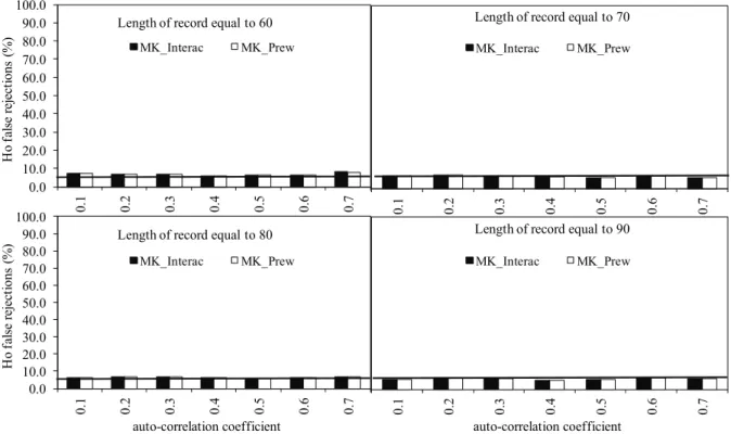
From Figure 1, it is clear that both the MK approaches show (approximately) the same rejection rate of true H0. Furthermore, considering SS equal to or greater than 70, the frequencies of occurrence of type I errors were virtually equal to the nominal significance level (5%) at which the MK were carried out. Therefore, based on these results and considering SS ≥ 70, both the

MK_interac and the MK_prew were capable of effectively limiting the influence of serial correlation on the occurrence of type I errors. In other words, considering the goal of this study, we may assume that the performance of the MK_interac was as good as the performance of the MK_prew in not rejecting a true H0. The results obtained when SS was set equal to 100 and 110 were virtually equal to those obtained when SS was set equal to 90 (not shown here for the sake of brevity). It is worth emphasizing that the results depicted in Figure 1 indicate that the pre-whitening approach is an important improvement in the use of the Mann-Kendall test. Thus, the study of Von Storch and Navarra (1995) may be seen as an important reference for the use (and understanding) of this trend test.

Finally, it is worth mentioning that when SS was set equal to 60 and r was set equal to 0.7, the rejection rates were slightly greater than the nominal

significance level (6.38% for both MK approaches; Figure 2). Moreover, when SS was set equal to 30, 40, and 50, the rejection rates obtained from both MK approaches were greater than the adopted significance level (not shown here for the sake of brevity). For instance, the highest rejection rates (8.06% for

MK_Interac and 7.52% for MK_Prew) were observed when SS and r were set equal to 30 and 0.7, respectively. To the best of the authors’ knowledge, the natural interpretation of this last feature is that the sample sizes equal to 30, 40 and 50 were not capable of providing reliable experimental results. Thus, no further analysis based on these lengths of records will be shown. The results obtained from SS = 60 and r = 0.7 should be treated with caution.

Type II errors

There are two fundamental ideas associated with the MK_interact algorithm. The first idea is that the estimation of serial correlation coefficients is influenced by the presence of a trend in the sample data. Consequently, the removal of a positive auto-correlation from a given series before carrying out a trend analysis (pre-whitening) may lead to a false reduction of the significance of a true trend (BURN et al., 2004; YUE et al., 2002 and 2003). Thus, under this first assumption, the “pre-whitening approach” should be avoided, as it may lead to a reduction of the power of the test.

0.0 10.0 20.0 30.0 40.0 50.0 60.0 70.0 80.0 90.0 100.0

0.1 0.2 0.3 0.4 0.5 0.6 0.7

H

o

f

als

e

re

je

ct

io

n

s

(%

)

Length of record equal to 60

MK_Interac MK_Prew

0.1 0.2 0.3 0.4 0.5 0.6 0.7

MK_Interac MK_Prew

0.0 10.0 20.0 30.0 40.0 50.0 60.0 70.0 80.0 90.0 100.0

0.1 0.2 0.3 0.4 0.5 0.6 0.7

H

o

f

al

se

rej

ect

io

n

s

(%

)

auto-correlation coefficient Length of record equal to 80

MK_Interac MK_Prew

0.1 0.2 0.3 0.4 0.5 0.6 0.7

MK_Interac MK_Prew

(5)

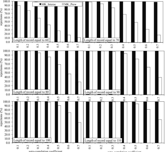
In spite of this influence of the trend on the autocorrelation estimation, the second idea rests on the assumption that the blended series (described in section 2) preserves the true trend. Therefore, because the Monte Carlo simulations were carried out based on this idea, one might expect that the values obtained from equation 4 should be similar to the trends that were superimposed on each simulated series. In other words, the sen-slope (obtained from the blended series) must properly estimate the trends that were superimposed on the original auto-correlated series. To the best of the authors’ knowledge, Yue et al. (2002) is the first study to provide empirical evidence for the validity of this second idea.The results depicted in Figures 2 to 6 also seem to support these two ideas. Figures 2

to 5 clearly indicate that the MK_interac was more powerful than the MK_prew.

As can be noted from Figures 2-5, the MK_interac

outperformed the MK_prew in all Monte Carlo

simulations. In addition, considering the highest values of r, the MK_prew performed poorly for all trend values. For instance, considering SS = 100, r = 0.7, and trend = 0.005, the MK_prew was able to indicate the presence of a trend in only 46% of the cases. Considering the same values of SS, r, and trend, the

MK_interac detected the presence of significant trends in all cases. Therefore,the results depicted in Figures 2 to 5 support the idea that the aforementioned pre-whitening approach leads to a reduction of the power of the MK test. These last results concur with the results obtained by Yue et al. (2002).

Length of record equal to 60 0.0 10.0 20.0 30.0 40.0 50.0 60.0 70.0 80.0 90.0 100.0 0. 1 0. 2 0. 3 0. 4 0. 5 0. 6 0. 7 H o fa ls e re je ct io n s (%

) MK_Interac MK_Prew

0. 1 0. 2 0. 3 0. 4 0. 5 0. 6 0. 7

Length of record equal to 100 0.0 10.0 20.0 30.0 40.0 50.0 60.0 70.0 80.0 90.0 100.0 0. 1 0. 2 0. 3 0. 4 0. 5 0. 6 0. 7 auto-correlation coefficient H o fa ls e re je ct io n s (% )

0. 1 0. 2 0. 3 0. 4 0. 5 0. 6 0. 7 auto-correlation coefficient Length of record equal to 80

0.0 10.0 20.0 30.0 40.0 50.0 60.0 70.0 80.0 90.0 100.0 0. 1 0. 2 0. 3 0. 4 0. 5 0. 6 0. 7 H o fa ls e re je ct io n s (% )

0. 1 0. 2 0. 3 0. 4 0. 5 0. 6 0. 7

(6)

Figure 6 depicts all 10000 values obtained from equation 4 through the Monte Carlo simulations (SS = 70, r = 0.7, and trend = 0.002; 0.004). As can be seen, the sen-slope seems to correctly estimate the trend (0.002) that was superimposed on the auto-correlated series. A total of 9000 of the 10000 values remained within the interval [0.0015:0.0025]. When the trend was set equal to 0.004, 9000 of the 10000 values remained between 0.0031 and 0.0049. As expected for any trend analysis, the performance of the sen-slope improves as the sample size and the magnitude of the trend increase. For instance, considering SS = 110, r = 0.7 and trend = 0.002 and = 0.004, the aforementioned intervals are [0.0016:0.0024] and [0.0036:0.0044], respectively. Therefore, the results obtained from Figure 6 and

those previously shown all support the idea that the blended series preserves the true trend. This desirable feature has allowed the correct estimation of the significance of the trends that were superimposed on each simulated (original) series.

Finally, it must be emphasized that the Monte Carlo simulations were carried out considering solely a particular case of monotonic trends: the linear shape. Although the study of Yue and Pilon (2004) has provided empirical evidence indicating that the MK test is only slightly influenced by the shape of a monotonic trend, one may reasonably argue that further studies are still required to assess the power of the MK_interac under nonlinear trend conditions. However, in the following section, no assumption was made about the shape of the trends.

0.0 10.0 20.0 30.0 40.0 50.0 60.0 70.0 80.0 90.0 100.0

0.1 0.2 0.3 0.4 0.5 0.6 0.7

re

ject

io

n

s (

%

)

MK_Interac MK_Prew

0.1 0.2 0.3 0.4 0.5 0.6 0.7

0.0 10.0 20.0 30.0 40.0 50.0 60.0 70.0 80.0 90.0 100.0

0.1 0.2 0.3 0.4 0.5 0.6 0.7

re

je

ct

io

n

s (%)

0.1 0.2 0.3 0.4 0.5 0.6 0.7

0.0 10.0 20.0 30.0 40.0 50.0 60.0 70.0 80.0 90.0 100.0

0.1 0.2 0.3 0.4 0.5 0.6 0.7

re

je

ct

io

n

s (%)

0.1 0.2 0.3 0.4 0.5 0.6 0.7

(7)

0.0 10.0 20.0 30.0 40.0 50.0 60.0 70.0 80.0 90.0 100.0

0.1 0.2 0.3 0.4 0.5 0.6 0.7

re

je

ct

io

n

s (%)

MK_Interac MK_Prew

0.1 0.2 0.3 0.4 0.5 0.6 0.7

0.0 10.0 20.0 30.0 40.0 50.0 60.0 70.0 80.0 90.0 100.0

0.1 0.2 0.3 0.4 0.5 0.6 0.7

re

je

ct

io

n

s (%)

0.1 0.2 0.3 0.4 0.5 0.6 0.7

0.0 10.0 20.0 30.0 40.0 50.0 60.0 70.0 80.0 90.0 100.0

0.1 0.2 0.3 0.4 0.5 0.6 0.7

re

je

ct

io

n

s (%)

0.1 0.2 0.3 0.4 0.5 0.6 0.7

Figure 4. Rejection rates of 10000 simulated series obtained from two different approaches to calculating the Mann-Kendall test (at the 5% significance level). All simulated series incorporate a (temporal) trend component equal to 0.04.

Case of Study

Before analyzing Table 1, it is worth recalling that the commonly adopted rejection level associated with the use of the MK test (and with many other statistical tests) is either 5 or 10%. In this view, the results presented in Table 1 seem to agree with Yue et al. (2002) in the sense that the pre-whitening approach may lead to a false reduction of the significance of an existing trend. For instance, while the MK_interact has indicated, for the 2nd_{ten days of Jun, decreasing trends} associated with a p-value equal to 0.04, the

MK_prew outcome is associated with a p-value equal to 0.07.

A similar and, for agro-meteorological purposes, more important feature, can be observed in the 3rd ten days of January and October. As can be noted

from Table 1, only the MK_interact allows the identification of significant trends (evaluated at the 10% significance level) during these periods. Thus, considering the aim of this study, we may indicate that as verified in the previous section, the

MK_interact outperformed the MK_prew inassessing the significance of the trends.

Based on these last considerations, it may be noted that the result obtained from the

(8)

(2007) observed increasing trends in the number of consecutive dry days over the State of São Paulo. These authors indicated that these trends (which may be linked to a delay in the resumption of the rainy season) began after 1985. Concerning

the agricultural interests, the decreasing trends

observed during the 3rd_{ten days of October}

(Table 1) reveal an unfavorable temporal distribution of the P-EP values observed during the beginning of the crop growing seasons.

0.0 10.0 20.0 30.0 40.0 50.0 60.0 70.0 80.0 90.0 100.0

0.1 0.2 0.3 0.4 0.5 0.6 0.7

rej

ect

io

n

s (

%

)

MK_Interac MK_Prew

0.1 0.2 0.3 0.4 0.5 0.6 0.7

100 0 ₀ ₀ ₀ ₀ ₀ ₀ ₀ _0. _0. _0. _0. _0. _0. _0.

0.0 10.0 20.0 30.0 40.0 50.0 60.0 70.0 80.0 90.0 100.0

0.1 0.2 0.3 0.4 0.5 0.6 0.7

re

je

c

ti

o

n

s (%

)

0.1 0.2 0.3 0.4 0.5 0.6 0.7

0.0 10.0 20.0 30.0 40.0 50.0 60.0 70.0 80.0 90.0 100.0

0.1 0.2 0.3 0.4 0.5 0.6 0.7

re

je

c

ti

o

n

s (%

)

0.

1

0.

2

0.

3

0.

4

0.

5

0.

6

0.

7

Figure 5. Rejection rates of 10000 simulated series obtained from two different approaches to calculating the Mann-Kendall test (at the 5% significance level). All simulated series incorporate a (temporal) trend component equal to 0.05.

0 1000 2000 3000 4000 5000 6000 7000 8000 9000 10000 0

0.001 0.002 0.003 0.004

Se

n sl

ope

Length of record equal to 70 auto-correlation coefficient equal to 0.7

Superimposed trend equal to 0.002

Simulated Series

0 1000 2000 3000 4000 5000 6000 7000 8000 9000 10000 0.002

0.003 0.004 0.005 0.006

Se

n sl

op

e

Superimposed trend equal to 0.004

Simulated series Simulated series

Figure 6. Values obtained from equation 4 (sen slope) through the Monte Carlo Simulation. Length of record equal to 70

auto-correlation coefficient equal to 0.7 Superimposed trend equal to 0.002

(9)

Table 1. Two different approaches to calculating the Mann-Kendall test (MK_interac and MK_prew). The slopes of the trends are also shown (sen-slope). Weather station of Campinas (1948-2011), State of São Paulo, Brazil.

Difference between precipitation and potential evapotranspiration (P-ET)

10-day MK_interac p-value MK_prew p-value sen slope

1-Jan 1.30 0.19 1.30 0.19 0.56 2-Jan -0.50 0.61 -0.50 0.61 -0.27 3-Jan 1.78 0.08 1.63 0.11 0.62

1-Feb -1.10 0.27 -1.10 0.27 -0.39

2-Feb 0.14 0.88 0.14 0.88 0.06

3-Feb -1.08 0.28 -1.08 0.28 -0.26

1-Mar 0.11 0.91 0.11 0.91 0.05

2-Mar -0.40 0.69 -0.40 0.69 -0.11

3-Mar 0.14 0.89 0.14 0.89 0.04

1-Apr -0.89 0.38 -0.89 0.38 -0.14

2-Apr 0.38 0.70 0.38 0.70 0.03

3-Apr -1.01 0.31 -1.01 0.31 -0.08

1-May 1.15 0.25 1.15 0.25 0.14

2-May 0.30 0.77 0.30 0.77 0.03

3-May 1.78 0.08 1.77 0.08 0.16

1-Jun -1.32 0.19 -1.31 0.19 -0.12

2-Jun -2.02 0.04 -1.84 0.07 -0.13

3-Jun 0.93 0.35 0.92 0.36 0.05

1-Jul -2.25 0.02 -2.25 0.02 -0.10 2-Jul 1.52 0.13 1.54 0.12 0.10 3-Jul 0.90 0.37 0.90 0.37 0.07

1-Aug 0.13 0.89 0.13 0.89 0.01

2-Aug -0.70 0.48 -0.70 0.48 -0.04

3-Aug -0.16 0.88 -0.15 0.88 -0.01

1-Sep 0.57 0.57 0.57 0.57 0.08

2-Sep 0.78 0.44 0.78 0.44 0.09

3-Sep 1.01 0.31 1.01 0.31 0.14

1-Oct 0.91 0.36 0.90 0.37 0.19

2-Oct -1.44 0.15 -1.44 0.15 -0.34

3-Oct -1.73 0.08 -1.44 0.15 -0.45

1-Nov -0.25 0.80 -0.25 0.80 -0.05

2-Nov 0.74 0.46 0.73 0.47 0.14

3-Nov 1.08 0.28 1.08 0.28 0.25

1-Dec 0.00 1.00 0.00 1.00 0.00

2-Dec 0.78 0.43 0.78 0.43 0.21

3-Dec 0.31 0.76 0.40 0.69 0.16

Conclusion

The MK_interact is more powerful than the

MK_prew. Both the results obtained from Monte Carlo experiments and the results obtained from the P-EP series of Campinas, State of São Paulo-Brazil have allowed us to conclude that the MK_interac

outperformed the MK_prew in detecting the

presence of trends. It was verified that with the

MK_prew, one may incorrectly conclude that the P-ETP series is free from trends. However, regarding agricultural interests, the significant decreasing trends detected by the MK_interac during the beginning of the crop growing seasons may be linked to an unfavorable temporal distribution of the P-EP values.

References

BLAIN, G. C. Séries anuais de temperatura máxima média do ar no Estado de São Paulo: variações e tendências climáticas. Revista Brasileira de Meteorologia, v. 25, n. 1, p. 114-124, 2010.

BLAIN, G. C. Aplicação do conceito do índice padronizado de precipitação à série decendial da diferença entre precipitação pluvial e evapotranspiração potencial. Bragantia, v. 70, n. 1, p. 234-245, 2011a.

BLAIN, G. C. Considerações estatísticas relativas a seis séries mensais de temperatura do ar da secretaria de agricultura e abastecimento do Estado de São Paulo. Revista Brasileira de Meteorologia, v. 26, n. 2, p. 279-296, 2011b.

BLAIN, G. C. Cento e vinte anos de totais extremos de precipitação pluvial máxima diária em Campinas, Estado de São Paulo: análises estatísticas. Bragantia, v. 70, n. 3, p. 722-728, 2011c.

BLAIN, G. C. Totais decendiais de precipitação pluvial em Campinas, SP: persistência temporal, periodicidades e tendências climáticas. Ciência Rural, v. 41, n. 5, p. 789-795, 2011d.

BLAIN, G. C. Monthly values of the standardized precipitation index in the State of São Paulo, Brazil: trends and spectral features under the normality assumption. Bragantia, v. 71, n. 1, p. 122-131, 2012.

BLAIN, G. C.; PIRES, R. C. M. Variabilidade temporal da evapotranspiração real e da razão entre evapotranspiração real e potencial em Campinas, Estado de São Paulo. Bragantia, v. 70, n. 2, p. 460-470, 2011.

BURN, D. H.; ELNUR, A. H. Detection of hidrological trends and variability. Journal of Hydrology, v. 255, n. 255, p. 107-122, 2002.

BURN, D. H.; CUNDERLIK, J.; PIETRONIRO, A. Hydrological trends and variability in the Liard river basin. Hydrological Sciences, v. 49, n. 1, p. 53-67, 2004. CHANDLER, R. E.; SCOTT, M. E. Statistical methods for trend detection and analysis in the environmental analysis. Chichester: John Wiley and Sons, 2011.

DUFEK, A. S.; AMBRIZZI, T. Precipitation variability in Sao Paulo State, Brazil. Theoretical and Applied Climatology, v. 93, n. 3/4, p. 167-178, 2007.

KENDALL, M. A.; STUART, A. The advanced theory of statistics. 2nded. Londres: Charles Griffin, 1967. MANN, H. B. Non-parametric tests against trend. Econometrica, v. 13, n. 3, p. 245-259, 1945.

MINUZZI, R. B.; CARAMORI, P. H.; BORROZINO, E. Tendências na variabilidade climática sazonal e anual das temperaturas máxima e mínima do ar no Estado do Paraná. Bragantia, v. 70, n. 2, p. 471-479, 2011.

PEREIRA, A. R.; ANGELOCCI, L. R.; SENTELHAS, P. C. Agrometeorologia: fundamentos e aplicações práticas. Guaíba: Agropecuária, 2002.

(10)

STRECK, N. A.; GABRIEL, L. F.; HELDWEIN, A. B.; BURIOL, G. A.; DE PAULA, M. G. Temperatura mínima de relva em Santa Maria, RS: climatologia, variabilidade interanual e tendência histórica. Bragantia, v. 70, n. 3, p. 696-706, 2011.

VON STORCH, H.; NAVARRA, A. Analysis of Climate Variability: Applications of Statistical Techniques. Berlin: Springer, 1995.

WILKS, D. S. Statistical methods in the atmospheric sciences. 2nd ed. San Diego: Academic Press, 2006.

YUE, S.; PILON, P. A comparison of the power of the t test, Mann-Kendall and bootstrap tests for trend detection. Hydrological Sciences Journal, v. 49, n. 49, p. 53-37, 2004. YUE, S.; PILON, P.; PHINNEY, B. Canadian streamflow trend detection: impacts of serial and cross-correlation. Hydrogical Sciences Journal,v. 48, n. 1, p. 51-64, 2003.

YUE, S.; PILON, P. J.; PHINNEY, B.; CAVADIAS, G. The influence of autocorrelation on the ability to detect trend in hydrological series. Hydrogical Processes, v.16, n. 16, p. 1807-1829, 2002.

ZHANG, X.; VINCENT, L. A.; HOGG, W. D.; NIITSOO, A. Temperature and precipitation trends in Canada during the 20th century. Atmosphere Ocean, v. 38, n. 3, p. 395-429, 2000.

Received on July 5, 2012. Accepted on February 9, 2013.