Página | 145
https://periodicos.utfpr.edu.br/rbpd
Hydraulic studies and their influence for
regional urban planning: a pratical approach
to Fynchal’s rivers
ABSTRACT
Dénio Gouveia Miranda
University of Madeira (UMa), Funchal, Portugal.
Rafael Freitas Camacho
[email protected] University of Madeira (UMa), Funchal, Portugal.
Sérgio Lousada
University of Madeira (UMa), Funchal, Portugal.
Rui Alexandre Castanho
University of Extremadura, Badajoz, Spain.
Flood phenomena in urban territories are a reality all over the globe.However, both urban planning processes and hydraulic studies are mostly not well-developed, considering the multidisciplinarity and complexity of the theme, resulting in urban agglomerations - with a tendency to occur in this typology of events – showing several gaps, regarding a well-developed and articulated urban planning, not being able to deal with this type of natural phenomenon.In this regard, the combining of multivariate studies, such as urban planning and hydraulic studies, are seen as critical to achieve a sustained territorial success of the regions affected by this typology of phenomena. Thus, by exploratory tools and analysis methods: i.e. calculation of roughness coefficients in artificial runoff channels, analysis of surface runoff, computer models, evaluation and analysis of design and spatial planning policies in urban areas, and its application to a case study - the case of the Funchal´s Rivers, Madeira, Portugal - are just a few examples of analysis that the study carries out, from a multidisciplinary perspective, in order to define bases and measures, enabling to prevent and minimize the negative impacts of such events, as well as increasing the safety of resident populations.
KEYWORDS: Artificial channels; Modeling; Multidisciplinary studies; Urban floods; Urban planning.
Página | 146
INTRODUCTION
Urban floods are a global event, with media cases around the globe as Dresden, Germany (Kreibich&Thieken, 2009), Genoa, Italy (Faccini, et al., 2014), the Caribbean (Acevedo-Espinoza, 2014) and the Autonomous Region of Madeira (RAM), target of several flood events, with the most recent being 20 February 2010 (Baioni, 2011; Oliveira, et al., 2011).
The relevance of a correct roughness coefficient defining for a given channel is pivotal for the proper assessment of drainage capacity. In this regard, an excessive value is uneconomical resulting in the poor design for the channel. By the other hand, a low value may result in a hydraulically unsuitablechannel. So, correct values of roughness coefficient are goals of a continuous research, resultingin a large amount of data, regarding this controversial issue (Harun-ur-Rashid, 1990; ACPA, 1997; IHB, 2005; Lencastre & Franco, 2006; Xing, et al., 2016).
In this sense, the variation of the coefficient of roughness can lead to increased/decreased downstream discharge, avoiding flooding; changes in the flow speed, which can prevent sedimentation of debris or wear and also the channel erosion; water level disparities; or cross-section geometric changes.Thus, the knowledge of the nature and state of channel features - i.e.roughness degree, pivotalregarding the considerable effect on the flow(Harun-ur-Rashid, 1990; ACPA, 1997; IHB, 2005; Lencastre & Franco, 2006; Xing, et al., 2016).The same goes for the roughness coefficient values obtained in laboratory tests for artificial channels correspond to values significantly lower than those corresponding to the actual scenario – i.e. do not consider the sediment transport, degradation of the coating of the walls and the riverbed and flow variation (Harun-ur-Rashid, 1990; ACPA, 1997; IHB, 2005; Lencastre& Franco, 2006; Xing, et al., 2016).
Usually, methods of direct measurement of flow rates in channels (of this typology) are not viable, particularly in flood events, steep slopes (greater than 1%) and sediment transport;once, the equipment is not prepared for such situations. In this regard, becomes necessary the use of indirect methods for a proper calculation of flow rates and consequent evaluation ofroughness coefficient; aspect that contributes to the difficulty in determining precisely the value of this coefficient (Harun-ur-Rashid, 1990; ACPA, 1997; IHB, 2005; Lencastre & Franco, 2006; Xing, et al., 2016). The coefficient can be found in tables collected by multiple authors, based on many studies, and may serve as a starting point for a new study. Still, may suffer considerable variation depending on the on-site conditions (Harun-ur-Rashid, 1990; ACPA, 1997; IHB, 2005; Lencastre & Franco, 2006; Xing, et al., 2016).
In this regard, the present study aims to evaluate the variation ofroughnesscoefficientdepending on thegeometric features, transported water volume and coating degradation of the channel, applying the chosen methodology to the case study of Funchal’s Rivers, at RAM.Thus, critical goals have been considering: defining methods of roughness coefficient calculating, specially designed for the evaluation of this parameter in the case of artificial channels, disregarding the effect of solid transport (not supported by the physical model); modelling the effects on values of the roughness coefficient depending on the geometry of the channel and flow rates; adopting practical criteria for evaluating the coefficient of roughness.
Página | 147
METHODOLOGY
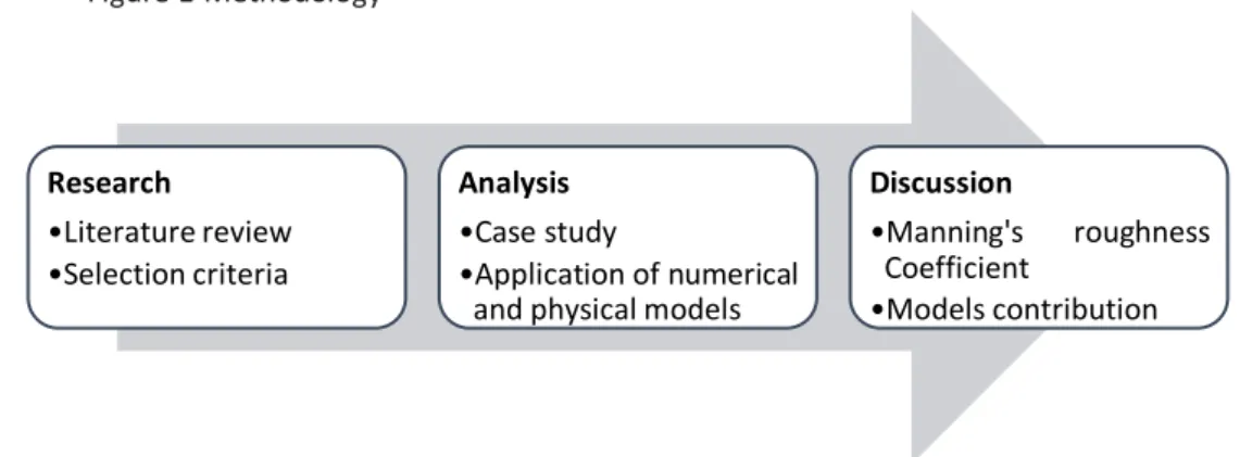
The used methodology (Figure 1), contemplates the adoption of a quantitative approach in the process of data collection and in its assessment, through statistical techniques, often applied to the sciences in descriptive studies. These techniquesseeks to find and classify the relationship between variables, based on information obtained from a case study analysys method (Yin, 1994; Levy, 2008), ideal for hydraulic studies (Amador, 2010).
Figure 1-Methodology
Literature review
Despite the difficulty in determining the coefficient of roughness, several scientificdocuments such as books, articles and studies have been published over the years (Harun-ur-Rashid, 1990; ACPA, 1997; Martins, 2000; Lyra, 2003; IHB, 2005; Abayati, et al., 2006; Szydłowski & Magnuszewski, 2007; De Doncker, et al., 2009; Hossain, et al., 2009; Baioni, 2011; Acevedo-Espinoza, 2014; Aupoix, 2015; Li, et al., 2015; Neal, et al., 2015; Cienciala & Hassan, 2016; Dimitriadis, et al., 2016; Verschoren, et al., 2016; Wei, et al., 2016), contributing to a significant improvement in applied methods, methodologies and materials, focusing not only technical aspects but also their influence in urban planning processes.
Cross-section
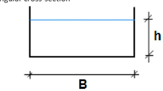
In the case of channels flows, the knowledge of the flow cross-section (perpendicular to the direction of the flow) is pivotal for the determination of the roughness coefficient and consequent flow characterization (Martins, 2000; IHB, 2005; Lencastre & Franco, 2006). The studied channels have a rectangular cross-section (Figure 2), giving emphasis to its discrimination.
Research •Literature review •Selection criteria Analysis •Case study •Application of numerical and physical models
Discussion
•Manning's roughness
Coefficient
Página | 148
Figure 2 - Rectangular cross-section
Cross-section features: (i) Depth, h: distance between the lowest point of the cross-section of the channel and the free surface of the liquid; (ii) width, B: distance between left and right margin, measured on the surface; (iii) wet area: cross-section area perpendicular to the direction of the flow (A = B.h); (iv) wet perimeter, P: length of the contour line of the wet area (P = B+2h); (v) hydraulic radius,RH: ratio between wet area and wet perimeter (RH= A/P).
PEAK FLOW RATES
The flow rate value it’s important to determine the value of the roughness coefficient, once by itself and depending on its change, leads to different water heights and velocities, resulting in different roughness coefficients. It’s in the interest of this study assess the peak flow rate for different return periods, obtaining a more assertive roughness coefficient and its effect during a flood event (Martins, 2000; IHB, 2005; Lencastre & Franco, 2006). Also, the peak flow rate can be determined from: empirical formulas-taking into account the application experience gained over the years and the watershed area; cinematic formulas - based on the concepts of time of concentration and critical precipitation (precipitation that originates the maximum peak flow rate for a given time of concentration); statistical formulas- regarding the analysis of a set of values for a given section (Martins, 2000; IHB, 2005; Lencastre & Franco, 2006).
Roughness coefficient
The flow conditions and the nature of a water line -i.e. roughness degree, greatly influences the flow (Harun-ur-Rashid, 1990; ACPA, 1997; Secretaria de Vias Públicas, 1999; Martins, 2000; Lyra, 2003; IHB, 2005; Abayati, et al., 2006; Lencastre & Franco, 2006; De Doncker, et al., 2009). Thus, a channel with good and regular maintenance, with smooth riverbanks andriverbed, for a given flow rate (Q) will drain with an average speed (U) which exceed considerably the value that would be obtained if the flow occurred on a natural one with the same dimensions, with roughed riverbanks and riverbed, due to inadequate maintenance. In the last case the flow resistance is much higher than the initially described, which causes a slowing of the flow (Harun-ur-Rashid, 1990; ACPA, 1997; Secretaria de Vias Públicas, 1999; Martins, 2000; Lyra, 2003; IHB, 2005; Abayati, et al., 2006; Lencastre & Franco, 2006; De Doncker, et al., 2009).
Then, the phenomenon will cause a rise of the water level in relation to the riverbed, becoming dangerous - mainly in the case of stone and rock channels
Página | 149
without maintenance, or containing vegetation or other materials(Harun-ur-Rashid, 1990; ACPA, 1997; Secretaria de Vias Públicas, 1999; Martins, 2000; Lyra, 2003; IHB, 2005; Abayati, et al., 2006; Lencastre & Franco, 2006; De Doncker, et al., 2009). The same goes for the study of free surface flows in uniform regime, Manning’s formula is applied, due to itsform simplicity and satisfactory results in practical applications, with the following formulation(Harun-ur-Rashid, 1990; ACPA, 1997; Secretaria de Vias Públicas, 1999; Martins, 2000; Lyra, 2003; IHB, 2005; Abayati, et al., 2006; Lencastre & Franco, 2006; De Doncker, et al., 2009):
𝑄 = (1 𝑛) ∙ 𝐴 ∙ 𝑅 2 3⁄ ∙ √𝑖 (eq. 1) Where: (Q) flow rate (m3/s); (A)flow cross-section (m2); (R)hydraulic radius (m);
(i)to reduced water heights: slope of the channel sill; to significant water heights: unitaryhead loss;
(n) Manning’sroughness coefficient (m-1/3).
During the design process, roughness coefficient selection should reflect the expected behavior of the structure throughout its lifetime, ensuring that, during this period, the flow capacity is equal or greater than that of the project. Commonly its applied standardized roughness coefficient values in drainage projects. Special situations should be analyzed by the designer, whom must justify the obtained values (Secretaria de ViasPúblicas, 1999; IHB, 2005; Abayati, et al., 2006). So, if the roughness characteristics of walls or riverbanksare different from the riverbed (mixed section), the "n" value obtained experimentally represents a weighted average - i.e. roughness coefficient must be composed from the roughness obtained for each applied material (Lencastre & Franco, 2006; De Doncker, et al., 2009).Thus, under different experimental conditions we can get different values of n, due to the influence of the walls increasing with the water height, therefore, the variation of cross-section (Harun-ur-Rashid, 1990; ACPA, 1997; Secretaria de ViasPúblicas, 1999; Martins, 2000; Lyra, 2003; IHB, 2005; Abayati, et al., 2006; Lencastre& Franco, 2006; De Doncker, et al., 2009).
According to the Secretaria de Vias Públicas(1999), between the different existing formulas for calculating the composite roughness is recommended the Horton-Einstein formula: 𝑛 = [∑ 𝑃𝑖𝑛𝑖 3 2⁄ 𝑁 1 𝑃 ] 2 3⁄ (eq. 2) Where:
Página | 150
(Pi) section “i” wet perimeter (m);
(ni) section “i” roughness (m-1/3).
The main obstacle when using this formulation lies in the definition of the roughness coefficient (n), since there is no exact methodology for its selection. Currently, the determination of a value of "n" is based on estimates of the flow resistance in the channel, because, in fact, the roughness coefficient is very variable and depends on a number of factors (Table 1) (Harun-ur-Rashid, 1990; ACPA, 1997; Secretaria de Vias Públicas, 1999; Martins, 2000; Lyra, 2003; IHB, 2005; Abayati, et al., 2006; Lencastre & Franco, 2006; De Doncker, et al., 2009).
Table 1- Crucial factors (adapted from Secretaria de Vias Públicas,1999; Lyra, 2003)
Factors Influence
Surface roughness Thin materials cause a minor effect, reducing the value of the coefficient; coarse
materials increase the roughness.
Vegetation Can be analyzed as a superficial roughness and the effect mainly depends on the
height, density, distribution and species, with special attention to its growth.
Channel irregularity Channels with wet perimeter irregularities and variations in cross-section suffer
an increase in roughness.
Sedimentation and erosion
The sedimentation of thin material in irregular channels can improve its surface, reducing roughness; the erosion may cause irregularities, increasing the roughness.
Obstructions The presence of tree trunks, pillars of bridges and other materials increase the
roughness of the channel, as well as the reduction of the section.
Channel Alignment Referring to curves; the smoother the curve (wide radius of curvature) the lower
the value of "n".
Size and shape of the channel Depending on the case, an increase in the hydraulic radius can increase or
decrease the coefficient of roughness.
Flow rate and water height In most flows the value of "n" decreases with the increase of the flow rate and
water height, for the same geometry and slope conditions.
Study area General
The Madeira Archipelago consists of three islands, being the largest with an area of approximately 22 km × 57 km (Figure 3). The volcanic mountains are positioned in a mountain range oriented in the direction Northwest-Southeast through the central portion of the island. The main peaks reach 1818 m (Pico Arieiro), 1852 m (Pico das Torres) and 1861 m (Pico Ruivo). The highlands extend laterally from the peaks (> 1000 m), deeply carved by water lines that flow into the sea. The highlands are more pronounced in West direction. To the East, the land is dry, windswept and deserted. The climate changes from subtropical to alpine forest along the mountains sides(França & Almeida, 2003; Ribeiro & Ramalho, 2009; Brum da Silveira, et al., 2010; Ramalho, et al., 2015; Pullen, et al., 2017).
Página | 151
Figure 3 - RAM relief chart (source: Wikimedia Commons)
Case study analysis
The case study refers to 3 rivers of municipality of Funchal: Sao João, Santa Luzia and João Gomes, (along the river mouth); for each of the streams was selecteda portion of 25 meters in length and applied the same methodology for different flow rate values, according to the selected return period (10, 50 and 100 years), to observe the variation of the roughness coefficient and its effect on flow. The three selected portions (each set between 2 sections) are thoroughly executed in concrete, i.e. walls and riverbed (Table 2).
Table 2 - Selected sections
ID Section Cross section elevation (m) Mileage (km) Width (m) Slope (%)
Position Left Center Right
SJ SJ1 Top 14.14 - 14.45 0+275 11.0 2.70 Riverbed 4.65 3.99 3.33 SJ0 Top 14.19 - 14.19 0+300 Riverbed 3.97 3.31 2.65 SL SL1 Top 11.42 - 10.28 0+125 14.0 3.05 Riverbed 5.08 5.08 5.08 SL0 Top 10.77 - 9.93 0+150 Riverbed 4.32 4.32 4.32 JG JG1 Top 9.47 - 9.17 0+200 10.0 2.00 Riverbed 0.84 0.84 0.84 JG0 Top 8.87 - 8.51 0+225 Riverbed 0.34 0.34 0.34
To analyse the selected portionsit’s important to characterize the watershed where they are inserted, obtaining important parameters for the calculation of peak flow rates, in an expedited and relatively simple manner, using the software ArcMap 10.3, main component of ArcGIS system (geographic information system) from the company ESRI (Environmental Systems Research Institute), mainly used to view, edit, create and analyse geospatial data, complemented with the support of a spreadsheet and CAD software, obtaining the parameters required for the 3 watersheds: Sao João, Santa Luzia and João Gomes (Figure 4).
Página | 152
Figure 4- Slope chart
From a geological perspective, Funchal consists essentially of superior complex layers, intermediate (highest percentage) and sedimentary cover (at the river mouth): local lava spills with tephra, between a million and six thousand years, extrusive igneous rocks; intermediate complex - lava sequences with tephra, separated by erosion levels, age between 1 and 2.5 million years, extrusive igneous rocks; sedimentary cover - riverine and marine sedimentary-gravels, mudslides, beach sands, and sedimentary rocks (França & Almeida, 2003; Ribeiro & Ramalho, 2009; Brum da Silveira, et al., 2010; Ramalho, et al., 2015; Pullen, et al., 2017).
Based on the land-use plan for the Funchal´s municipality, which represents the model of spatial planning according to the classification and qualification of soils, the study area is essentially urban (area along the river mouth) Regarding the vegetal sphere, the vegetation is composed of ground cover plants found, mainly, in urban green spaces and on the banks and bottom of riversides - presence of flexible vegetation, except for the areas where the riverbed is covered by concrete.
Página | 153
Roughness coeficiente analysis
The practical process of analysis of the roughness coefficient starts with the precipitation analysis, followed by the calculation of flow rates, application of numerical models and physical model, ending with the technical analysis of the hydraulic behavior and discussion of the obtained results.
Precipitation analysis
Consists in a process of adjustment of statistical laws to the hydrological variables samples and estimation of these variables as a function of the probability of exceedance (Figure 5).
Figure 5- Probabilistic Analysis
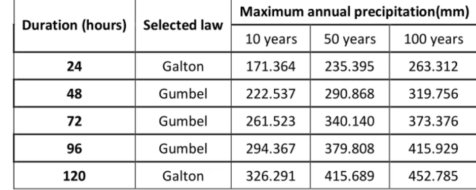
The sample consists of daily precipitation data, by a station, to the Funchal´s municipality, for a series of 15 years ending in 31/12/2014, obtained by consulting the website of National Information System of Water Resources (SNIRH). Thus, for study purposes, it was chosen the return periods of 10, 50 and 100 years by considering that corresponds to the design of an artificial channel at short, medium and long-term, respectively (Table 3).
Table 3- Maximum annual precipitation for a given duration, statistical law and return period
Duration (hours) Selected law Maximum annual precipitation(mm)
10 years 50 years 100 years
24 Galton 171.364 235.395 263.312
48 Gumbel 222.537 290.868 319.756
72 Gumbel 261.523 340.140 373.376
96 Gumbel 294.367 379.808 415.929
120 Galton 326.291 415.689 452.785
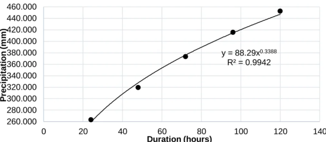
Based on pairs of values (duration, precipitation) and laws selection, for each of the considered return periods, the Line of Pluviometric Possibility (LPP) is defined(Figure 6). Sample Statistics Statistical laws Laws selectio n Precipitati on values LPP
Página | 154
Figure 6- LPP for a return period of 100 years
Through the analysis of the LPP, along with formula selection, it is possible to calculate the precipitation values and, consequently, their intensity.
Peak flow rates
For the values obtained for each of the different formulas, is determined the average value (Table 4) that, for each return period time, is used for the purposes of calculation, simulation, and modeling.For these formulas were adopted values for the coefficients (Table 5).
Table 4- Peak flow rates
Peak flow rates for the study cases Return
period (years)
Watershed São João Santa Luzia João Gomes
Formulas Peak flow rate (m³/s)
10 Forti 131.459 127.895 114.501 Iskowski 195.885 190.247 169.225 Pagliaro 408.555 397.973 357.961 Racional 479.874 480.863 444.855 Giandotti 167.270 167.615 155.064 Mockus 345.468 347.811 323.729 Témez 227.401 227.870 210.807 Average 244.489 242.534 222.018 50 Forti 131.459 127.895 114.501 Iskowski 195.885 190.247 169.225 Pagliaro 408.555 397.973 357.961 Racional 900.465 904.454 839.402 Giandotti 261.564 262.722 243.826 Mockus 345.468 347.811 323.729 Témez 355.592 357.167 331.478 Average 324.873 323.534 297.515 100 Forti 131.459 127.895 114.501 Iskowski 195.885 190.247 169.225 Pagliaro 408.555 397.973 357.961 Racional 1097.566 1103.333 1025.115 Giandotti 306.064 307.672 285.861 Mockus 345.468 347.811 323.729 Témez 416.089 418.276 388.623 Average 362.636 361.651 333.127 y = 88.29x0.3388 R² = 0.9942 260.000 280.000 300.000 320.000 340.000 360.000 380.000 400.000 420.000 440.000 460.000 0 20 40 60 80 100 120 140 P re c ip it a ti o n ( m m ) Duration (hours)
Página | 155
Table 5-Adopted values for the coefficients present in the used formulas Adopted values
Formulas Parameter São João Santa Luzia João Gomes
Iskowski kis 0.600 0.600 0.600 mi 8.878 8.889 8.931 Racional C 0.70 0.70 0.70 Cf, T=10 1.00 1.00 1.00 Cf, T=50 1.20 1.20 1.20 Cf, T=100 1.25 1.25 1.25 Giandotti λ 0.24 0.24 0.24 Témez C 0.995 0.995 0.995 P0 1.162 1.162 1.162 CN 95.000 95.000 95.000 CNIII 97.763 97.763 97.763 Modeling
The area of modeling and simulation, it’s an important feature and indispensable tool to the scientific method for testing and validation of concepts and theories, used in virtually all Civil Engineering projects.
The construction of a model serves to better understand the system, helping to show the system as it is or how we wish it to be, allowing specification of the structure or the behavior of a system, providing a guide to build the system and even documents the decisions were taken.
For this purpose, it’s applied numerical and/or physical models (commonly referred to as experimental models). For this particular study, it was applied 1 physical model (multi-purpose flume) and 2 numeric models (programmed spreadsheet and HEC-RAS software).
RESULTS
The results obtained through the program HEC-RAS will be disregarded since they refer to a situation which the value of the roughness coefficient keeps constant along the length of the channel when in reality it varies.Also, is referred only the portion of 25.0 m of João Gomes river, is that this analysis is similar to that of the other two sections, such as its conclusions.
The variation of roughness coefficient has been studied taking into account different flow rates for each return period (10, 50 and 100 years) that, in the case of João Gomes river, take the values of 222,018, 297,515 and 333,127 m3/s,
respectively, which in the experimental model corresponds, respectively,to 6,000, 8,000 and 9,000 m3/h obtained through the rule of three,fixing the maximum real
flow rate to the maximum flow rate allowed by the equipment, while on the programmed spreadsheetapplies the real flow rates. Nevertheless, should be taking into account that the results obtained through the experimental model must be analyzedregardingeventual factory imperfections and even the
Página | 156
imperfections of the channel, justifying in advance the exaggerated variations of coefficient along the canal (Figure 7).
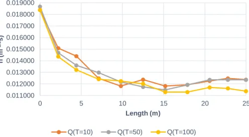
Figure 7 - Variation of roughness coefficient for different flow rates in the João Gomes river
Despite the errors, the previous graph does not escape the rule of the coefficient "n" decreasing along the channel, because the water height decreases, producing less friction between the walls of the channel, favoring a faster flow. Pump fluctuations that cause the water line to beunstable, non-uniform geometric reductions, imperfection in the bottom of the channel and reduced flow rates are an accumulation of small errors that significantly influence the results.
The programmed spreadsheet can make a detailed analysis of the variation of the roughness coefficient, only needing an initial value to start the iteration. In these graphs it is possible to take two relevant notes:
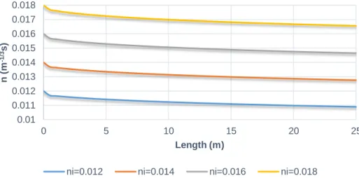
1. For the same flow rate, the higher the initial value of "n", the lower the final value of it (larger the difference between the initial and final values). This is due to the fact that theunitary head loss decreases more rapidly to greater initial values of "n" (Figure 8 and Table 6).
0.011000 0.012000 0.013000 0.014000 0.015000 0.016000 0.017000 0.018000 0.019000 0 5 10 15 20 25 n ( m -1 /3s) Length (m) Q(T=10) Q(T=50) Q(T=100)
Página | 157
Figure 8 - Variation of roughness coefficient with distinct ni, for Q(T=100) inJoão
Gomes river
Table 6- Difference between the initial and final values of "n" for a constant flow rate Q(T=100) ni nf Difference 0.012 0.010895301 0.001104699 0.014 0.012760373 0.001239627 0.016 0.014646424 0.001353576 0.018 0.016557249 0.001442751
2. For the same initial value of "n", the greater the flow, the higher the final value of the roughness coefficient (lesser the difference between the initial and final values). This is explained by the water height increasing with the increase of the flow rate (Figure 9 and Table 7).
Figure 9 - Variation of roughness coefficient with ni=0.018, for distinct flow rates
inJoão Gomes river
Table 7 - Difference between the initial and final values of "n" fora constant "ni"
value Caudal ni nf Difference Q(T=10) 0.018 0.016344482 0.001655518 Q(T=50) 0.018 0.016498506 0.001501494 Q(T=100) 0.018 0.016557249 0.001442751 0.01 0.011 0.012 0.013 0.014 0.015 0.016 0.017 0.018 0 5 10 15 20 25 n ( m -1 /3s) Length (m)
ni=0.012 ni=0.014 ni=0.016 ni=0.018
0.0162 0.0164 0.0166 0.0168 0.017 0.0172 0.0174 0.0176 0.0178 0.018 0 5 10 15 20 25 n ( m -1 /3s) Length (m) Q(T=10) Q(T=50) Q(T=100)
Página | 158
Both in Figure 8 as in Figure 9 it’s visible a slight variation (sudden decrease in the value of "n") between 0 m and 0.5 m in length. Such variation is due to the start-up of the program that generates an initial value of "n" slightly higher, because the indication given by the user, required to start up, is that the flow starts from the critical height, when in fact the flow begins at the top of the watershed, arriving at this section with a given height which, without field measurements, it is necessary to arbitrate. As the flow is fast, it’s conditioned by the upstream height, having the user to give that information to the program through the critical height calculation. The sudden variation in starting the program is equivalent to the situation, in physics, in which to move a given object that is initially in the state of rest is needed an extra bit of force needed for it to move.
DISCUSSION AND CONCLUSIONS
Throughout the study were adopted three different methods to characterize the roughness coefficient and evaluate its effect on the flow in artificial channels, emphasizing the importance of the programmed spreadsheet, as the method from which obtained the best results (ACPA, 1997; Hossain, et al., 2009; Aupoix, 2015; Dimitriadis, et al., 2016).
The lack of measurements of water heights for use in HEC-RAS program and the results obtained through experimental model makes two of the best methods appear inefficient, when in fact only were subject to the circumstances of the moment attesting the potentiality of them (ACPA, 1997; Hossain, et al., 2009; Aupoix, 2015; Dimitriadis, et al., 2016).
The results obtained through the experimental model were not in accordance with the expected(or at least not fully9, in this regard that were expected errors, but not to the point of not being able to make a correlation with the other two methods. Demonstrates the need for an experimental model created from scratch, although costly, would result in more feasible and satisfactory results (ACPA, 1997; Hossain, et al., 2009; Aupoix, 2015; Dimitriadis, et al., 2016).
By the other hand, modelling in HEC-RAS program was dependent on the prior existence of water height values measured in rivers(which did not exist), in those sections in order to simulate the flow and it wouldn't make sense to make use –i.e. values generated by the programmed spreadsheet calculation since it’s subject to the assumption of an initial value of roughness coefficient from which all others are calculated (ACPA, 1997; Hossain, et al., 2009; Aupoix, 2015; Dimitriadis, et al., 2016).
Thus, the spreadsheet was the method that produced the best results allowing to verify that the coefficient "n" decreases along the channel, due to the decrease of water height, producing less friction between the water and the walls of the channel, favoring a faster flow. Still, for the same flow rate, the higher is the initial value of "n", the lower the final value of the same (a larger difference between the initial and final values). This happens because the unitary head loss decreases more rapidly to greater initial values of "n"; and for the same initial value of "n", the greater the flow rate, the higher the final value of the roughness
Página | 159
coefficient (lesser difference between the initial and final values) (ACPA, 1997; Hossain, et al., 2009; Aupoix, 2015; Dimitriadis, et al., 2016).
Based on the results, the HEC-RAS program just overcomes the spreadsheet, about the evaluation of roughness coefficient, when in the presence of water height measurements allowing (after calibration) a simulation more realistic than the spreadsheet. The experimental model works best when the dimensions, materials and flow rates are reproducible with a real-like behaviour, otherwise it becomes very difficult to interpret the results obtained in the model and its impact on the assessment of the real case(ACPA, 1997; Hossain, et al., 2009; Aupoix, 2015; Dimitriadis, et al., 2016).
The research, enable to conclude that the roughness coefficient andwater volume flow in an artificial channel affect each other making the section geometry asignificant role in balancing the two(ACPA, 1997; Hossain, et al., 2009; Aupoix, 2015; Dimitriadis, et al., 2016).Thus, it is advised that close tourban agglomerations, cultivated fields or other important infrastructure, measures like: enlargement of the cross-section and/or deepening of the channel, executed based on materials that produceminor friction forces allowing the flow, focusing on flood events, to stay in the channel and process rapidly in these situations with minor turbulence, thereby ensuring the safety of inhabitants and existing infrastructures. Such measures will depend on the sensitivity of local governments to this issue, focusing mainly on a correct planning and spatial planning, an essential tool in the prevention of extreme phenomena (Baioni, 2011; Acevedo-Espinoza, 2014; Faccini, et al., 2014; Neal, et al., 2015; Castanho et al., 2016).
Página | 160
Estudos hidráulicos e a sua influência no
planejamento urbano regional: aplicação
prática às ribeiras do Funchal
RESUMO
Fenómenos de cheias em territórios urbanos são uma realidade um pouco por todo o globo. Contudo, quer os processos de planeamento urbanístico, quer os estudos hidráulicos, maioritariamente, não são elaborados, tendo em consideração, a multidisciplinaridade e complexidade da temática, resultando em aglomerações urbanas – com tendência à ocorrência desta tipologia de evento – que apresentam lacunas de um correto planeamento urbano articulado, não estando capacitadas para fazer face a este tipo de fenómeno natural.Nesse sentido, a articulação de estudos multivariados, como são o caso do planeamento urbano, e hidráulicos, são vistos como essências para o sucesso territorial sustentado das regiões afetadas por esta tipologia de fenómenos. Assim, através de ferramentas exploratórias e de análise, como disso são exemplo: o cálculo coeficientes de rugosidade em canais de escoamento artificiais, análise de escoamentos superficiais, modelos computorizados, avaliação e análise do design e políticas de ordenamento territorial em áreas urbanas, e a sua aplicação a um caso prático – o caso das ribeiras da cidade do Funchal, Madeira, Portugal – são apenas alguns exemplos de análise que o estudo leva a cabo, desde uma perspetiva multidisciplinar, a fim de definir bases e medidas para poder prevenir e minimizar os impactos negativos de tais eventos, assim como aumentar a segurança das populações residentes.
PALAVRAS-CHAVE: Canais de escoamento artificiais; Cheias urbanas; Modelação; Multidisciplinaridade; Planeamento urbanístico.
Página | 161
REFERÊNCIAS
Abayati, M. A., Yusuf, B., Mohammed, T., & Ghazali, A. (2006). Manning roughness coefficient for grass-lined channel. Suranaree Journal of Science and
Technology, 317-330.
Acevedo-Espinoza, S. (2014). Debt, Growth and Natural Disasters A Caribbean Trilogy. IMF Working Papers. doi:10.5089/9781498337601.001
ACPA. (1997). História da pesquisa dos valores do coeficiente de Manning. (ABTC, Trad.) ACPA.
Amador, M. d. (2010). Tipos de métodos científicos. Lisboa: FCSH, Universidade Nova de Lisboa. Obtido de
http://www.fcsh.unl.pt/docentes/cceiaold/images/stories/disciplinas/PhD%20Di dactica%20LE/tipos_met_cientificos.pdf
Aupoix, B. (2015). Revisiting the Discrete Element Method for Predictions of Flows Over Rough Surfaces. Journal of Fluids Engineering. doi:10.1115/1.4031558
Baioni, D. (2011). Human activity and damaging landslides and floods on Madeira Island. Natural Hazards and Earth System Sciences, 3035-3046.
doi:10.5194/nhess-11-3035-2011
Brum da Silveira, A., Madeira, J., Ramalho, R., Fonseca, P., Rodrigues, C., & Prada, S. (2010). Carta Geológica da ilha da Madeira na escala 1:50.000. Folha A e B. Região Autónoma da Madeira: Secretaria Regional do Ambiente e Recursos Naturais.
Castanho, R., Loures, L., Fernández, J., and Fernández-Pozo, L., (2016). Identifying
critical factors for success in Cross Border Cooperation (CBC) development projects. Habitat International.
Cienciala, P., & Hassan, M. A. (2016). Sampling variability in estimates of flow characteristics in coarse-bed channels: Effects of sample size. Water Resources
Research, 1899–1922. doi:10.1002/2015WR017259
De Doncker, L., Troch, P., Verhoeven, R., Bal, K., Meire, P., & Quintelier, J. (2009). Determination of the Manning Roughness Coefficient Influenced by Vegetation in the River Aa and Biebrza River. Environmental Fluid Mechanics, 549-567.
Página | 162
Dimitriadis, P., Tegos, A., Oikonomou, A., Pagana, V., Koukouvinos, A., Mamassis, N., . . . Efstratiadis, A. (2016). Comparative evaluation of 1D and quasi-2D
hydraulic models based on benchmark and real-world applications for uncertainty assessment in flood mapping. Journal of Hydrology, 478-492. doi:10.1016/j.jhydrol.2016.01.020
Faccini, F., Luino, F., Sacchini, A., & Laura, T. (2014). Flash Flood Events and Urban Development in Genoa (Italy): Lost in Translation. XII Congress "Engineering
Geology for Society and Territory". Turin: Springer International Publishing
Switzerland. doi:10.1007/978-3-319-09048-1_155
França, J. A., & Almeida, A. B. (2003). Plano regional de água da Madeira. Síntese
do diagnóstico e dos objectivos.
Harun-ur-Rashid, M. (1990). Estimation of Manning's roughness coefficient for basin and border irrigation. Em B. Clothier, W. Dierickx, J. Oster, & D. Wichelns (Edits.), Agricultural Water Management (1 ed., Vol. 18, pp. 29-33).
Hossain, A., Jia, Y., & Chao, X. (2009). Estimation of Manning's roughness coefficient distribution for hydrodynamic model using remotely sensed land cover features. 17th International Conference on Geoinformatics, Geoinformatics
2009 (pp. 1-4). Fairfax, Virginia, USA: George Mason University.
doi:10.1109/GEOINFORMATICS.2009.5293484
IHB. (2005). Manual on Hydrography. Monaco: International Hydrographic Bureau.
Kreibich, H., & Thieken, A. (2009). Coping with floods in the city of Dresden, Germany. Natural Hazards. doi:10.1007/s11069-007-9200-8
Lencastre, A., & Franco, F. M. (2006). Lições de Hidrologia 3ª edição revista. Lisboa: Fundação da Faculdade de Ciências e Tecnologia da Universidade Nova de Lisboa.
Levy, J. S. (2008). Case Studies - Types, Designs and Logics of Inference. Conflict
Management and Peace Science, 1-18. doi:10.1080/07388940701860318
Li, S., Shi, H., Xiong, Z., Huai, W., & Cheng, N. (2015). New formulation for the effective relative roughness height of open channel flows with submerged vegetation. Advances in Water Resources, 46-57.
Página | 163
Lyra, G. B. (2003). Avaliação experimental da ocorrência de vazão e velocidades
máximas em canais de secção circular. Minas Gerais, Brasil: Universidade Federal
de Viçosa. Obtido em 17 de março de 2017, de
http://alexandria.cpd.ufv.br:8000/teses/engenharia%20agricola/2003/177992f.p df
Martins, F. J. (2000). Dimensionamento hidrológico e hidráulico de passagens
inferiores rodoviárias para águas pluviais. Coimbra: Universidade de Coimbra.
Obtido em 10 de março de 2017, de
http://repositorio.ipv.pt/bitstream/10400.19/482/1/Tese%20-%20Mestrado.pdf
Neal, J. C., Odoni, N. A., Trigg, M. A., Freer, J. E., Garcia-Pintado, J., Mason, D. C., . . . Bates, P. D. (2015). Efficient incorporation of channel cross-section geometry uncertainty into regional and global scale flood inundation models. Journal of
Hydrology, 169-183. doi:10.1016/j.jhydrol.2015.07.026
Oliveira, R. P., Almeida, A. B., Sousa, J., Pereira, M. J., Portela, M. M., Coutinho, M. A., . . . Lopes, S. (2011). A avaliação do risco de aluviões na ilha da Madeira.
10º Simpósio de Hidráulica e Recursos Hídricos dos Países de Língua Oficial Portuguesa (10º SILUSBA) (pp. 1-20). IST, UMa & LREC. Obtido de
https://www.researchgate.net/publication/244994405
Pullen, J., Caldeira, R., D. Doyle, J., May, P., & Tomé, R. (2017). Modeling the air-sea feedback system of Madeira Island. Journal of Advances in Modeling Earth
Systems, 1-24. doi:10.1002/2016MS000861
Ramalho, R., Brum da Silveira, A., Fonseca, P., Madeira, J., Cosca, M., Cachão, M., . . . Prada, S. (2015). The emergence of volcanic oceanic islands on a slow-moving plate: The example of Madeira Island, NE Atlantic. Geochemistry Geophysics
Geosystems, 522–537. doi:10.1002/2014GC005657
Ribeiro, M. L., & Ramalho, M. (2009). Uma Visita Geológica ao Arquipélago da
Madeira. Lisboa: Direção Regional do Comércio, Indústria e Energia e Laboratório
Nacional de Energia e Geologia, I. P.
Secretaria de Vias Públicas. (1999). Diretrizes de Projeto para Coeficiente de
Rugosidade. São Paulo: Perfeitura do Município de São Paulo. Obtido em 17 de
março de 2017, de
http://www.prefeitura.sp.gov.br/cidade/secretarias/upload/infraestrutura/NOR MAS%20T%C3%89CNICAS%20INSTRU%C3%87%C3%95ES%20NOVAS/Hidr%C3%A 1ulica%20e%20drenagem%20urbana/DH-H13.pdf
Szydłowski, M., & Magnuszewski, A. (2007). Free surface flow modeling in numerical estimation of flood risk zones: a case study. Task Quaterly, 301-313.
Página | 164
Verschoren, V., Meire, D., Schoelynck, J., Buis, K., Bal, K. D., Troch, P., . . . Temmerman, S. (2016). Resistance and reconfiguration of natural flexible submerged vegetation in hydrodynamic river modelling. Environmental Fluid
Mechanics, 245–265. doi:10.1007/s10652-015-9432-1
Wei, M., Blanckaert, K., Heyman, J., Li, D., & Schleiss, A. J. (2016). A parametrical study on secondary flow in sharp open-channel bends: experiments and
theoretical modelling. Journal of Hydro-environment Research, 1-13. doi:10.1016/J.JHER.2016.04.001
Xing, Y., Yang, S., Zhou, H., & Liang, Q. (2016). Effect of Floodplain Roughness on Velocity Distribution in Mountain Rivers. Procedia Engineering, 467-475.
doi:10.1016/j.proeng.2016.07.539
Yin, R. K. (1994). Case Study Research: Design and Methods.London: SAGE Publications.
Recebido: 07 out. 2017.
Aprovado: 04 nov. 2017.
DOI: 10.3895/rbpd.v7n1.7179
Como citar: MIRANDA, D. G.; CAMACHO, R. F.; LOUSADA, S.; CASTANHO, R. A. Hydraulic studies and
their influence for regional urban planning: a pratical approach to Fynchal’s rivers. R. bras. Planej.
Desenv.,Curitiba, v. 7, n. 1, p. 145-164, jan./abr. 2018. Disponível em: <https://periodicos.utfpr.edu.br/rbpd>.
Acesso em: XXX.
Correspondência:
Rui Alexandre Castanho
Avda. de Elvas, s/n, 06071 Badajoz, Espanha
Direito autoral: Este artigo está licenciado sob os termos da Licença CreativeCommons-Atribuição 4.0