Media mix modeling: a case study on optimizing television and digital media spend for a retailer

i

Media Mix Modeling

José Francisco Sá Marques Rocha

A Case Study on Optimizing Television

and Digital Media Spend for a Retailer

Work project presented has partial requisite to obtain the

Master’s degree in Information Management

ii

NOVA Information Management School

Instituto Superior de Estatística e Gestão de Informação

Universidade Nova de Lisboa

MEDIA MIX MODELING:

A CASE STUDY ON OPTIMIZING TELEVISION AND DIGITAL MEDIA SPEND FOR A RETAILER

por

José Francisco Sá Marques Rocha

Work project presented has partial requisite to obtain the Master’s degree in Information Management, with specialization in Marketing Intelligence

Orientador/Coorientador: Diego Costa Pinto Coorientador: Manuel Vilares

iii

ACKNOWLEDGMENTS

Grateful for the support of my family and friends throughout these years while I was working in the fast-paced digital marketing agency industry and studying at NOVA Information Management School at the same time. I will certainly give back soon.

iv

ABSTRACT

Retailers invest most of their advertising budget in traditional channels, namely Television, even though the percentage of budget allocated towards digital media has been increasing. Since the largest part of sales still happen in physical stores, marketers face the challenge of optimizing their media mix to maximize revenue.

To address this challenge, media mix models were developed using the traditional modeling approach, based on linear regressions, with data from a retailer’s advertising campaign, specifically the online and offline investments per channel and online conversion metrics.

The models were influenced by the selection bias regarding funnel effects, which was exacerbated by the use of the last-touch attribution model that tends to disproportionately skew marketer

investment away from higher funnel channels to lower-funnel. Nonetheless, results from the models suggest that online channels were more effective in explaining the variance of the number of

participations, which were a proxy to sales.

To managers, this thesis highlights that there are factors specific to their own campaigns that influence the media mix models, which they must consider and, if possible, control for. One factor is the selection biases, such as ad targeting that may arise from using the paid search channel or remarketing tactics, seasonality or the purchase funnel effects bias that undermines the contribution of higher-funnel channels like TV, which generates awareness in the target audience. Therefore, companies should assess which of these biases might have a bigger influence on their results and design their models accordingly.

Data limitations are the most common constraint for marketing mix modeling. In this case, we did not have access to sales and media spend historical data. Therefore, it was not possible to

understand what the uplift in sales caused by the promotion was, as well as to verify the impact of the promotion on items that were eligible to participate in the promotion, versus the items that were not. Also, we were not able to reduce the bias from the paid search channel because we lacked the search query data necessary to control for it and improve the accuracy of the models.

Moreover, this project is not the ultimate solution for the “company’s” marketing measurement challenges but rather informs its next initiatives. It describes the state of the art in marketing mix modeling, reveals the limitations of the models developed and suggests ways to improve future models. In turn, this is expected to provide more accurate marketing measurement, and as a result, a media budget allocation that improves business performance.

KEYWORDS

media mix modeling; marketing mix modeling; marketing mix effectiveness; marketing budget allocation; budget allocation optimization; marketing mix

v

INDEX

1. Introduction ... 1

2. Literature Review ... 4

2.1. Measurement Approaches: Media Mix Modeling and Multi-touch Attribution ... 4

2.2. Unified Measurement ... 5

2.3. Marketing Mix Modeling ... 6

2.3.1.Evolution ... 6

2.3.2.Data Requirements ... 8

2.3.3.Challenges and Opportunities ... 8

2.3.4.Alternatives to Marketing Mix Models ... 11

2.4. Attribution ... 11

2.4.1.Rules-based Models ... 11

2.4.2.Algorithmic Models ... 12

2.4.3.Online to Offline Attribution ... 12

2.4.4.Multi-touch Attribution Challenges ... 15

3. Methodology ... 16

3.1. Dataset Description ... 16

3.2. Measurement and Modeling Approach ... 17

3.3. Media Mix Models ... 18

4. Implications and Discussion ... 22

4.1. Linear Regressions ... 22

4.2. Residuals ... 25

4.3. Performance by Day of the Week ... 26

5. Conclusions ... 29

5.1. Managerial Contributions ... 30

5.2. Limitations and Recommendations for Future Research ... 31

vi

INDEX OF FIGURES

Figure 1 - Marketing mix modeling and multitouch attribution. Source: (Gartner, 2018) ... 4

Figure 2 - Unified measurement. Source: (Analytics Partners, 2019b) ... 6

Figure 3 – Retailer’s customer journey example (Interactive Advertising Bureau, 2017) ... 14

Figure 4 – Carryover effect of advertising (Tellis, 2006) ... 20

Figure 5 - Residuals of the model with the highest adjusted r-squared ... 25

vii

INDEX OF TABLES

Table 1 - Models with the highest adjusted r-squared ... 22 Table 2 - P-values of the model32_Participations_01234567 ... 23 Table 3 - Coefficients of the models with the highest adjusted r-squared ... 24

viii

LIST OF ACRONYMS AND ABBREVIATIONS

MTA Multi-touch attribution assigns credit to multiple touch points along the path to conversion. Conversely, the last-touch model only gives credit to the last interaction before the user took the desired action of the campaign.

KPI A Key Performance Indicator is a measurable value that demonstrates how effectively a company is achieving key business objectives.

TV Television.

CRM Customer relationship management is an approach to manage a company's interaction with its current and potential customers. It is often referred to as the technology platform used for that approach.

GDPR General Data Protection Regulation is a regulation in European Union law on data

protection and privacy.

ANOVA Analysis of variance is a statistical technique that is used to check if the means of two or

1

1. INTRODUCTION

Marketing leaders reported that their biggest C-suite communication challenge was to prove the impact of marketing on financial outcomes (American Marketing Association, Deloitte, & Fuqua School of Business, 2019). Chief Marketing Officers are being asked to prove the value of their rising 1 trillion-dollar investments but are struggling to keep up with an increasingly more complex marketing mix, technology ecosystem, and customer journey. Thus, measuring and optimizing the contribution of marketing to enterprise value has emerged as a critical topic for senior leaders (Forbes & Marketing Accountability Standards Board, 2018).

Measuring the return on marketing is often less precise than the measurements of other business activities. However, marketing leaders are increasingly required to demonstrate the financial impact of their actions so that they can show accountability for business results, gain the respect of other business leaders, and secure future investment (Harvard Business Review, 2019). In fact, over half of the Chief Financial Officers reported attaching a high priority to measuring return on marketing in the following three years (Forbes & Marketing Accountability Standards Board, 2018).

One of the largest dairy companies in Brazil wants to improve the measurement of its marketing activities. The “company” allocates most of its media spend towards TV advertising while the remaining goes to online channels, but sales happen in physical stores. Therefore, the question that guides this research is: how can the “company” optimize the media mix between online and offline channels to maximize in-store sales? As a solution, this paper suggests media mix modeling, which is a time-tested method for measuring the impact of marketing. It is how leading brands figure out what is working across channels, so they can adapt media budgets accordingly (Hartman, 2019). To get a better understanding of this research question is important to aware of the stakeholders involved. First, the “company”, whose name cannot be revealed because of a Non-disclosure agreement, is one of the largest dairy companies in Brazil that sells over 100 different products, mainly in physical stores. Between 65 to 70 percent of its media budget is allocated towards offline channels, mostly TV advertising, whereas the rest is invested in online channels. Second, a

“marketing agency” is looking for ways to improve the measurement of its media campaigns and optimize budgets accordingly. However, when the success of an online marketing campaign depends on selling products in a physical store, measuring the impact of the campaign becomes challenging. Therefore, a “consulting firm” specialized in data science, partnered with NOVA Information

Management School to help the “company” measure the effectiveness of media spend across online and offline channels in driving in-store sales during a promotion.

At the end of 2018, the “marketing agency” ran a promotion on behalf of the “company”. To

participate, consumers had to purchase in physical stores a set of products eligible in the promotion, then sign up or log in to their account on the internet and enter the IDs present in the receipts from the in-store purchases. Participations were the number of sets of products registered online. In turn, each participation gave the user the opportunity to win prizes, which were randomly given in drafts. Consequently, the more times someone bought products in-store and participated online, the higher the probability of winning prizes.

In this campaign, the measurement of the impact of each media channel on sales was a challenge. Having access to the online and offline investments per channel and online conversion metrics of the

2 campaign, by day, media mix models were developed. These models are used to understand how media spend affects sales and to optimize the media budget allocation to get the optimal media mix (Jin, Wang, Sun, Chan, & Koehler, 2017). In this project, online conversion metrics such as

Participations, which is the number of sets of products registered online, were used as a proxy to sales.

Before exploring the theme of media mix models, is vital to provide context into the media landscape in Brazil, to better interpret decisions made throughout the project. In Brazil, there is a gap between the opportunity that digital marketing represents and the level of maturity in this discipline. Also, media budget allocation between traditional and digital media lags the evolution in consumer behavior (McKinsey & Associação Brasileira de Anunciantes, 2019). Even though that 67% of media investment in the country was allocated towards offline media channels in 2018, companies planned to invest more 30% in digital media in 2019 relatively to the previous year (Interactive Advertising Bureau Brasil, PwC, & Ilumeo, 2019). However, shifting budgets from traditional media to digital is not enough. Companies need to become more mature in four digital marketing dimensions: 1) Processes, People and Culture, 2) Data and Technology, 3) Customer Journey and Experience and 4) Measurement (McKinsey & Associação Brasileira de Anunciantes, 2019). This project is a step forward for the “company” in the Measurement dimension.

Digital channels play an important role in Brazil. It is the second country in the world where people spend more time per day surfing on the internet. On average, Brazilians spend nine hours and 29 minutes on the web, which is much higher than the world’s average of 6 hours and 42 minutes (Hootsuite & We Are Social, 2019). Additionally, Facebook is expected to reach half of the population by 2021 (Statista, 2019), whereas the country has the second largest user base on Instagram (Reuters, 2018). Besides that, the internet penetration rate is forecasted to grow to about 61% in 2021, up from 56.8% in 2016 (Statista, 2019). Nonetheless, TV is the dominant media channel in the country since 93% of the population in the main metropolitan regions watch television

regularly and 56% keep themselves informed through this medium (Kantar Ibope, 2018).

However, digital and offline channels are becoming intertwined in the country. For instance, 51% of those who consume their news online do it through websites or apps owned by traditional media companies. From those that access the internet while they watch TV, 23% engage on social media about the content they are watching on television (Kantar Ibope, 2018) and only 18% of consumers declare to pay exclusive attention to TV, whose percentage dropped by almost 25% over 3 years (Google, 2018). Even when purchases happen offline, digital media impacts consumer’s purchase decisions. In fact, 55% of consumers search for new brands or products online before they make an offline purchase. In the food and beverage category, despite only 4% made their last purchase online, 17% would rather prefer to buy online and 33% browse the internet for new products or brands before purchasing them in physical stores (BCG, 2018).

As a result, retailers are developing omni-channel initiatives such as enabling in-store pickup of online orders, shipping products from several stores/shipment centers or by showing accurate inventory online. Moreover, multi-channel shoppers spend, on average, 15% to 30% more than the other customers (IDC, 2017).

3 This article is organized as follows. Section 2 is a literature review of the measurement approaches utilized by marketers to address the challenges in gauging campaign performance when online and offline channels are used.

Section 3 outlines the methodology utilized during the project. It describes the dataset, explains why

linear regressions were the modeling approach chosen and provides the rationale for the media mix models developed.

Section 4 discusses the most important findings throughout the thesis.

Section 5 succints the main conclusions of the thesis, describes the contributions for managers, lays

out the limitations faced during the project and provides recommendations for future researchers or marketers that aim to develop media mix models.

4

2. LITERATURE REVIEW

2.1.

M

A

:

M

M

M

M

-

A

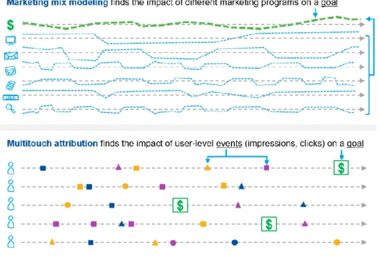
Marketing mix modeling and multitouch attribution (MTA) are two solutions that measure the impact of marketing and media efforts and suggest ways to optimize their marketing performance (Gartner, 2018).

Figure 1 - Marketing mix modeling and multitouch attribution. Source: (Gartner, 2018) Marketing mix models help to measure how advertising spend affects sales and to guide budget allocation to get the optimal marketing mix (Jin et al., 2017). These are statistical models that use aggregate historical data to model sales over time, as a function of advertising variables, other marketing variables or even control variables like weather, seasonality, and competition (Chan & Perry, 2017). This data typically includes media spend across digital and offline channels, such as TV and print. It is a top-down approach that measures the high-level impact of a range of marketing tactics. They are used to guide investment decisions by showing how channel performance

compares. Marketing mix models that only include media-related data are called media mix models (Gartner, 2018).

Attribution is the process of determining the relative contribution of individual campaign impressions towards a goal for the purpose of performance measurement and optimization. The dominant attribution methodology is last-touch, which assigns credit to only the last ad that a consumer interacted with, before taking the desired action of the campaign (Interactive Advertising Bureau, 2017). In this case, the desired action of the campaign was for users to participate online by registering a set of products they had bought in physical stores. However, the last-touch model is flawed because individuals are usually exposed to multiple advertising channels before making any

5 purchasing decision. Therefore, a fundamental problem in measuring advertising effectiveness is to quantify how revenue should be attributed to multiple touch-points along consumers' conversion paths, which is the sequence, timing, and engagement in advertising channels along the purchase funnel (Zhao, Mahboobi, & Bagheri, 2019).

MTA is a solution for this measurement challenge since it assigns credit to multiple touch points along the path to conversion. By assembling information about user characteristics, media touch points, and sales/conversion data, marketers can understand which combination of channels, audience targets, publishers, devices, creatives, search keywords, or other marketing considerations are performing most effectively against their Key Performance Indicator (KPI). Thus, they are widely regarded by practitioners as a proxy for optimizing campaign performance (Interactive Advertising Bureau, 2017). Contrary to media mix modeling, it is a bottom-up measurement approach that requires individual-level data (Gartner, 2018).

Marketing mix modeling is most useful when sales happen in physical stores, and media is allocated towards online and offline channels. On the other hand, MTA is preferred when the conversion path happens mostly online, and marketers have user-level data readily available (Gartner, 2018).

2.2.

U

M

By combining both approaches, marketers can further corroborate which channels are contributing to the pre-defined KPIs while preventing misguided conclusions when gaps between these two methods arise. For instance, a marketer may use MTA to determine the relative contributions of display and paid search tactics to online revenue. Meanwhile, they may also use marketing mix modeling to estimate the impact of those same tactics on offline sales. Blending the detailed view from MTA with the higher-level analysis provided by marketing mix modeling, companies gain more accurate measurements. However, the different data sources and levels of data capture make the automated reconciliation of the two approaches difficult. As a result, some providers offer custom unified measurement solutions (Gartner, 2018).

Analytics Partners, a Google Measurement Partner, is one of the consulting firms that offer this custom solution. The output from unified measurement is a holistic view with consistent data and incrementality, leading to a unified version of the truth (Analytics Partners, 2019b).

6 Figure 2 - Unified measurement. Source: (Analytics Partners, 2019b)

As the customer journey becomes more complex, so does measuring marketing performance. Traditional marketing mix modeling does not deliver insights in real-time or integrate with business intelligence tools. It guides yearly or quarterly budget allocations but does not provide the timely and actionable insights across channels that modern marketers need. With tools like Google Attribution 360, part of the Google Analytics 360 Suite, advertisers can benefit from both the top-down analysis of marketing mix modeling and the bottom-up analysis of data-driven attribution—all within one integrated tool. Data-driven attribution model reveals the value of each digital touchpoint in the customer journey so that marketers can improve performance on-the-fly. On the other hand, Attribution 360 gives marketers the holistic insights of marketing mix modeling analysis across channels. This methodology provides a more actionable and accurate understanding of the complete marketing mix (Google, 2016). However, integrating online with offline media spend data is still a challenge for these platforms.

2.3.

M

M

M

2.3.1. Evolution

Marketing Mix, also known as the 4Ps (Product, Price, Place, Promotion), was a marketing management framework popularised by McCarthy in the 60s. Based on consumer behavior and company objectives, a marketer aims to develop the “right” product, makes it available at the “right” place with the “right” promotion and at the “right” price, to satisfy target consumers and meet the business’ goals (McCarthy, 1960).

In the following three decades researchers have reported a large number of econometric studies on the price sensitivity of select demand (Tellis, 1988). In the 80s, retailers started to use point-of-sales UPC scanners, which provided the granular and time-based sales data that marketing mix models need. However, during the 90s, challenges to collect media-related data emerged. On one hand, the growth in satellite and cable transmission gave people a wider variety of video content to consume, reducing the size of the audiences per show. This caused difficulty in measuring exposure to

7 was the adoption of the Internet, which created new, difficult-to-measure touch points that

influenced consumer purchases (Fulgoni, 2018).

Econometric models that measured the impact of media on sales were enhanced according to seven patterns of response to advertising. Those patterns were named current, shape, competitive, carryover, dynamic, content and media effects (Tellis, 2006). Recently, two research articles

incorporated the carryover and shape effects on their marketing mix models (Jin et al., 2017; Wang, Jin, Sun, Chan, & Koehler, 2017). The carryover or lag effect is the impact that occurs in time periods following the pulse of advertising, which may be because of delayed consumer response, delayed purchase due to consumer’s inventory, or purchases from customers who have heard from those who first saw the ad. The shape effect suggests that investing very low amounts in advertising might not be effective because ads get drowned out in the noise, whereas it also has diminishing returns, meaning, the growth of spend might not increase sales because the market could be saturated or consumers suffer from tedium with repetitive ads (Tellis, 2006).

With the rise of big data, a novel way to fit a marketing mix model is presented by (Saboo, Kumar, & Park, 2016). A time-varying effects model used big data to explicitly account for the temporal variations in consumer responsiveness to the direct marketing efforts of a Fortune 500 company, which aimed to improve marketing return-on-investment on a real-time basis, thus allowing a more frequent reallocation of marketing resources.

Over the past few years, fitting models using a Bayesian framework has been a suggested

methodology by researchers. In one study, (Jin et al., 2017) estimated the models using a Bayesian approach to consider the carryover and diminishing returns, which are hard to capture using linear regressions. Also, (Wang et al., 2017) pooled data from several brands within the same product category to get more observations and greater variability in media spend patterns. After, they used a hierarchical Bayesian approach to improve the media mix model of this dataset. Additionally, (Sun, Wang, Jin, Chan, & Koehler, 2017) proposed a geo-level Bayesian hierarchical model when sub-national data is available, which can provide estimates with tighter credible intervals compared to a model with national-level data alone.

Often, companies collaborate with marketing analytics firms to implement marketing mix models. These firms provide both the expertise from consultants and technology to simulate and optimize media budget allocations. One of these companies is Visual IQ, a Nielsen company. Their process to build a marketing mix model starts with collecting data on marketing spend and sales performance. After, they enrich the dataset with proprietary and third-party data. Then, they build regression models to determine how marketing tactics (independent variables) relate to outcomes like sales (dependent variables). Finally, consultants analyze results and provide actionable insights. Moreover, they allow marketers to simulate and optimize budget allocation through an online platform (Visual IQ, 2019). Similarly, the consulting firm Analytics Partners forecasts, monitors and periodically assesses the impact of newly executed marketing plans. A digital platform provides marketers with key model insights, dashboards and tools for planning and optimization of media budgets (Analytics Partners, 2019a).

8

2.3.2. Data Requirements

Data used to fit marketing mix models are typically historical weekly or monthly aggregated national data, although geo-level data can be used. The data includes:

 response data, typically sales but can be other KPI

 media metrics by channel, such as impressions, clicks, GRPs, with the cost being the most commonly used

 marketing metrics such as price, promotion, product distribution  control factors such as seasonality, weather or competition.

The response data needs to be at the same level of granularity as the ads spend data. So, while an advertiser may have precise SKU level data, advertising is usually done at a brand or

product level over an entire country. For the response data, such as sales, advertisers have in place a robust data collection mechanism. However, media data is more challenging to collect, as ad

campaigns are often executed through several intermediaries, such as agencies or online platforms. Since it is difficult to get competitor variables for pricing, promotion, and distribution through third-parties, these variables are often omitted (Chan & Perry, 2017).

2.3.3. Challenges and Opportunities

2.3.3.1. Challenge 1: Data Limitations

The amount of data is often limited since a typical marketing mix modeling dataset that considers three years of national weekly has only 156 data points and is expected to produce a model with 20 or more ad channels. This quantity of data is normally insufficient to build a stable linear regression with 7-10 data points per parameter. Also, advertisers tend to allocate media budgets across channels in a correlated way. Hence, the input variables may be highly correlated which leads to coefficient estimates with a high variance that hinders the accuracy of the model. Additionally, companies normally have a historical range of ad spend according to their objectives but want to gather insights outside of their range of ad spend such as knowing what would happen if they doubled ad spend in the following year. This extrapolation with a limited range of data may lead to biased results (Chan & Perry, 2017).

One way to address these data limitations is to pool data from several brands within the same product category, introducing more data and independent variability into the models, and then, fitting the models using a hierarchical Bayesian approach (Wang et al., 2017). Using simulation and real case studies, the authors provide evidence that this approach can improve parameter estimation and reduce the uncertainty of model prediction and extrapolation. Another way to get a higher sample size and more independent variation in the dataset is to use sub-national data, if available, and fit the model using a hierarchical Bayesian approach. As a result, it generally provides estimates with tighter intervals compared to a model with only national-level data, which in turn reduces its

9 error. Moreover, if advertisers follow this approach, they can optimize their media budgets at the sub-national level desired (Sun et al., 2017).

2.3.3.2. Challenge 2: Selection Bias

Selection bias from ad targeting appears when an underlying interest or demand from the target population is driving both the ad spend and the outcome (Chen et al., 2018). This phenomenon has been mathematically described by (Varian, 2016).

Ad Targeting

When it comes to ad targeting, companies can target ads to people that had shown interest in their products. For instance, digital channels allow marketers to show ads if people have been to the company’s website, a tactic known as remarketing. The underlying demand for this remarketing audience that contributes to sales is not included in the model (Chan & Perry, 2017).

Another instance where ads are targeted to consumers that have shown interest in the company’s products is in paid search advertising. In this form of advertising, ads are tailored to the user’s queries on a search engine. To correct for this bias, (Chen et al., 2018) used causal diagrams of the search ad environment to derive a statistically principled method to estimate search ad ROAS, where search query data satisfied the back-door criterion for the causal effect of this type of advertising on sales. Also, control variables are an opportunity to reduce selection bias. To address paid search bias, search query volumes can be used as a control variable for the component of underlying demand from consumers likely to make product-related searches (Chen et al., 2018).

Seasonality

Another instance where selection bias arises is when media allocation varies according to the seasonality in demand and the effect is hard to capture using control variables (Chan & Perry, 2017).

Funnel Effects

Additionally, purchase funnel effects may lead to selection bias. As an example, a TV campaign might increase the number of search queries covered by the advertiser’s paid search strategy, which increases the volume in search queries. However, the model might attribute the sales to the paid search channel without giving any credit to the TV campaign (Chan & Perry, 2017). This bias is exacerbated by the dominant adoption of the last-touch attribution model, which assigns credit to only the last ad that a consumer interacted with, before converting, as mentioned in section 2.1.

Measurement Approaches: Media Mix Modeling and Multi-touch Attribution.

Graphical models are a suggested methodology to get a clearer understanding of the underlying causal structure of the purchase funnel, which may lead to a model that best captures the

conditional dependencies between media channels (Chan & Perry, 2017). A graphical model is a form of expressing dependencies between variables, both observed and unobserved (Pearl, 2009).

Another way to reduce biases from the purchase funnel effects is to develop a custom unified measurement solution, combining MTA with marketing mix modeling to get a single version of the truth, as mentioned in section 2.2. Unified Measurement. However, this solution is far-fetched to most companies due to its complexity and high cost.

10

2.3.3.3. Challenge 3: Model Selection and Uncertainty

The explanatory power of a few input variables is normally enough to build models with high accuracy metrics such as the R-squared or predictive error. This makes it easier to find models with high predictive accuracy by testing several specifications, but that might provide the advertiser with different conclusions regarding media budget allocation (Chan & Perry, 2017).

Simulation helps to test the reliability of several models with similar accuracy metrics under different assumptions. The outcome of the model such as ROAS is known under several scenarios, which can be compared to the ground truth. As described in section 2.3.1. Evolution, service providers like (Visual IQ, 2019) offer clients a way to simulate the impact of different media mixes on their desired outcome. Google Inc. has also been developing simulation tools capable of generating aggregate-level time series data related to marketing measurement (Zhang & Vaver, 2017).

2.3.3.4. Challenge 4: Modeling Approach

Even though linear regressions are the default modeling approach, fitting marketing mix models using a Bayesian approach has proven to have many benefits according to (Chan & Perry, 2017), such as the ability to:

 Use informative priors for the parameters, where the informative priors can come from a variety of sources

 Handle complicated models

 Report on both parameter and model uncertainty  Propagate uncertainty to optimization statements

Additionally, Bayesian approaches have been helpful to address the challenge in section 2.3.3.1.

Challenge 1: Data Limitations, either by pooling data from several brands within the same product

category (Wang et al., 2017) or by using sub-national data (Sun et al., 2017). Furthermore, (Jin et al., 2017) estimated marketing mix models using a Bayesian approach to consider the carryover and diminishing returns, which are hard to capture using linear regressions.

Traditional marketing mix models are less suitable when a firm aims to reallocate their marketing budgets on a real-time basis and faces a context of big data. Using a time-varying effects model that takes into account that marketing-mix effectiveness varies with the evolution of the consumer-brand relationship, (Saboo et al., 2016) provide support for the increase in revenue for a Fortune 500 retailer when performing dynamic marketing resource allocation by adopting their framework.

11

2.3.4. Alternatives to Marketing Mix Models

Marketing mix models are a common methodology by marketers to answer causal questions around their advertising. Even though there are other alternatives, they have significant drawbacks.

Randomized Experiments

Randomized experiments split a population by a test group and a control group, where no action is taken by the latter. If there is an observable difference between the outcomes of both groups, it can be caused by the action only performed by the test group. Some drawbacks of this approach are the technical hurdles in implementation, opportunity cost from having a control group, cost of having a test group or the requirement of a large sample size to draw statistically significant insights (Chan & Perry, 2017). Also, they are considered expensive and difficult to conduct at scale across multiple media (Jin et al., 2017). As an example, (Lewis & Reiley, 2014) measure the positive causal effects of online advertising for a major retailer through a randomized experiment with 1.6 million customers. Potential Outcomes Framework

The potential outcomes framework, also known as the Rubin causal model for causal inference, relies on historical data to derive causal conclusions. Though, in a common media mix modeling scenario, the number of data points is too low to satisfy the assumptions required by this approach (Chan & Perry, 2017).

2.4.

A

Attribution is the process of identifying a set of user actions across screens and touchpoints that contribute to a campaign’s desired outcome and then assigning value to each of these events (Interactive Advertising Bureau, 2016). Marketers use attribution to interpret the influence of advertisements on consumer behavior and to optimize campaigns accordingly (Nisar & Yeung, 2018).

2.4.1. Rules-based Models

Last-touch attribution, which assigns credit to only the last interaction that a consumer had with an advertiser before taking the campaign’s desired action, remains as the dominant attribution since the early days of digital advertising (Interactive Advertising Bureau, 2017).

This methodology is part of a category of models called rules-based models, which assign credit to multiple events along a path to conversion based on a predetermined set of rules. According to (Interactive Advertising Bureau, 2016), other rules-based models are:

 First-touch: opposite from the last-touch model, the first event recorded along the path to conversion receives 100% of the credit.

 Even Weighting: credit is applied equally across all events measured along a path to conversion.

 Time decay: credit is assigned to events at increasing or decreasing intervals along a path to conversion. For example, 40% of credit could be given to events within 24 hours of

12 conversion, 30% to events within 1-3 days, 20% to events within 3-7 days, and 10% to events within 7-14 days.

 U-shaped: credit is disproportionally assigned to events at the beginning and end of a path to conversion.

2.4.2. Algorithmic Models

As customer journeys become more complex, individuals are exposed to multiple advertising channels before making any purchase decision (Zhao et al., 2019). As a result, marketers need to get a better understanding of sales-cycle length and the impact of their activities over the purchase funnel, so that they can optimize campaigns accordingly (Nisar & Yeung, 2018). Therefore, last-touch attribution paints an increasingly more incomplete picture of the advertising value that each media touchpoint has along the path to conversion. In fact, this model runs counter to long-standing consumer psychology research that proved there are incremental gains to message recall associated with repeat exposure to advertising. Consequently, it tends to skew media investment away from higher-funnel channels that generate awareness towards the product or service offered, in detriment of lower-funnel channels (Interactive Advertising Bureau, 2017).

One alternative to rules-based models are algorithmic, multi-touch approaches, which assign credit to all events along a path to conversion given a computer-based, data-driven analysis (Interactive Advertising Bureau, 2016). Analysts claim that these approaches provide more accurate cost per acquisition figures per channel than traditional methods (Nisar & Yeung, 2018). In turn, this enables marketers to make decisions based on the influence of a channel on the final purchase, and not just whether that media touchpoint generated the final conversion.

To implement an algorithmic attribution model, companies can either build their own or rely on a platform. An instance of the former is the research developed by (Zhao et al., 2019), which used relative importance methods to quantify how revenue should be attributed to online advertising inputs. Also, they utilized simulations to demonstrate the superior performance of their algorithmic approach to traditional methods. On the other hand, a prominent example of the latter is the data-driven model of Google Analytics, which uses machine learning to determine how much credit should assign to each interaction in the user journey (Arensman, 2017). First, Google develops conversion probability models from available path data of the advertiser, to understand how the presence of marketing touchpoints impacts users’ probability of conversion. Then, it applies to this probabilistic dataset an algorithm based on a concept from cooperative game theory called the Shapley Value (Google, 2019a).

2.4.3. Online to Offline Attribution

Nowadays, one key challenge of attribution is to identify the same user across devices. In the early days of the Internet, browser cookies were used to determine when a user was exposed to paid messaging and if a user engaged with the ad unit in a specific way, as well as the events that took place along the path to conversion within a specific campaign. Multi-touch attribution eases

cross-13 device measurement by using device graphs (Interactive Advertising Bureau, 2016). These graphs describe how different devices relate to each other by mapping all the devices, IDs, and associated data back to one unique user or household (Neufeld, 2017). This approach is the foundation for a holistic view of message delivery within an omni-channel digital media campaign, enabling marketers to target users, not browser cookies (Interactive Advertising Bureau, 2016).

When the majority of sales happen offline, understanding how digital advertising contributes to revenue helps the advertiser to optimize its media activity. In the dairy sector, most of the

transactions still happen in-store. In fact, worldwide e-commerce sales in the dairy sector went from 3.4% in 2015 to 4.2% in 2017. Also, Brazil only accounted for 0.1% of the total Fast-Moving Consumer Goods e-commerce sales, as of 2017 (Kantar Worldpanel, 2018).

To attribute offline purchases to online behavior, marketers need to link several datasets (Interactive Advertising Bureau, 2017):

 User identity and characteristics: audience or device graphing data that aim to identify at the user-level specific interests, demographics, past purchase history with the business, web content and browsing behavior, as well as other information that might be relevant to inform advertising activities. This data can be obtained from the company’s Customer Relationship Management (CRM) system and acquired through third-party data partners. As mentioned before, device graphing data allows marketers to associate individuals with the various devices that they use.

 Media touchpoints: MTA models benefit by including as much information as possible about user engagement with advertising. However, when traditional media is used on a campaign, the entire truth of how the user consumes media cannot be captured entirely by the model, having to rely on assumptions and modeling.

 Sales/conversion data

If marketers can assemble the information about user characteristics, media touch points, and sales/conversion data into an MTA solution, they can begin to understand which combination of channels, audience targets, publishers, devices, creatives, search keywords, or other marketing considerations are performing most effectively against their KPI. This enables not only make optimization decisions to improve individual campaign performance over time but also uncovers insights that can inform future campaign planning and non-advertising related aspects of the business like packaging distribution, or operations (Interactive Advertising Bureau, 2017).

As an example, we can analyze the following hypothetical customer journey for a retailer’s new shirt line advertising campaign:

14 Figure 3 – Retailer’s customer journey example (Interactive Advertising Bureau, 2017)

The customer, called Michelle, visits the offline store to buy a few products and signs up for the loyalty card. At this moment, the company gathers transaction and sign up related data, such as Michelle’s e-mail address, phone number, customer ID, etc. that can be stored in a CRM. Then, she goes online and signs in on the retailer’s website across several devices, visiting pages related to the new shirt line. Thus, the company shows her several ads to entice Michelle to buy. She ends up adding to cart, but not purchasing. Later, she heads to the store and converts offline. By assembling the customer ID on the loyalty card with this purchase, the marketer can start to model which ads had the most impact on the buying decision.

Nonetheless, in most of the cases, companies do not have loyalty cards and/or the user does not sign in on their online account across several devices. Hence, device graphs become fundamental to link media consumption by device to the user or household. Even when companies can identify users across devices, they still cannot connect offline purchases to a certain individual. In this case, marketers track in-store foot traffic and associate it with other datasets. Attribution typically occurs by matching the cookie or device identifier linked to an ad exposure on a user’s device graph with location data, that can be gathered through several methods such as a location-based measurement provider or a physical beacon placed in-store (Interactive Advertising Bureau, 2016).

15

2.4.4. Multi-touch Attribution Challenges

Last-touch methodologies remain resilient despite its limitations. First, it runs counter to consumer psychology research that long ago established the value and incremental gains to message recall associated with repeat exposure (Interactive Advertising Bureau, 2017). Also, another drawback is that it does not consider vital interactions along the customer journey, unfairly rewarding lower-funnel channels (Nisar & Yeung, 2018).

Nevertheless, the strength of this model lies in its ability to determine which channels lead users to a final conversion, which infuses confidence into the efficacy of digital advertising campaigns (Nisar & Yeung, 2018). Hence, most of the web analytics and advertising platforms still use by default the last-touch model, requiring marketers to evaluate alternatives and change the attribution model. Often, implementing multi-touch attribution models can become complex and resource consuming. Marketers reported that walled gardens were the key challenge to implement a MTA solution (Mobile Marketing Association, 2017). Companies like Google, Facebook or Amazon seek to encompass as much consumer activity as possible inside their platforms, thereby attracting marketer’s media spending. However, they have the power to control the availability of user-level data to third parties (Fulgoni, 2018). In turn, this inhibits marketers from linking all ad serving and/or conversion data to user profiles, which compromises the completeness and accuracy of MTA (Mobile Marketing Association, 2019).

Last but not least, privacy regulations such as the General Data Protection Regulation (GDPR) have caused companies to tighten rules for sharing ad service along with matchable user IDs. One

prominent example of this restriction was that the industry-leading ad server, Google’s DoubleClick, stopped sharing user IDs as part of log files (Mobile Marketing Association, 2019). Even though there are a few alternatives, MTA became harder for advertisers. Alternatives include relying on Google’s data-driven attribution model, accessing encrypted user-level data on Ads Data Hub (Google’s data warehouse where ad exposure data is housed), using a different ad server or building a proprietary dataset using tags and pixels (Kihn, 2018). Also, privacy regulations reduced the information available around web-browsing cookies, IP addresses, e-mails and other data points that could be used for a more accurate MTA model (Interactive Advertising Bureau, 2017).

16

3. METHODOLOGY

3.1.

D

D

The following data regarding the promotion was available by day, in an Excel file:  Media amounts invested, broken down by each online and offline channel.  Online conversion metrics:

 Website Visits: number of visits to the website.

 Signups: number of users that signed up. Users could sign up without having bought any product or they may have already signed up in previous campaigns.

 Participants with Products: number of participants that registered at least a set of products.

 Participations: number of sets of products registered. Users could participate more than once.

The online conversion metric Participations is the better proxy to sales, making it the most relevant target variable for this project since the firm wants to know the impact of media investment on sales. Initially, daily spend on the online channel was separated by Facebook, YouTube, Google, and several websites. The investment in websites was aggregated into a channel called Display because the traffic generated through banner ads on websites is grouped by default into the channel grouping called Display in web analytics platforms such as Google Analytics (Google, 2019b).

During the promotion, 77.1% of the budget was allocated towards the offline channel. Within digital channels, Facebook was the one with the highest spend (43.2%), closely followed by Display (40.3%), then YouTube (8.3%) and Google Search (8.2%).

The offline spend was very high during the promotion because the “company” invested in a TV show that reaches a mass audience across Brazil, which is broadcasted on Sunday nights. Therefore, a spike in spending happens on Sundays, while the number of Participations does not rise immediately, because TV advertising has long-term effects. In fact, on Sundays, 93.3% of the investment was allocated towards offline, whereas the average investment during the campaign on television was 77.1%.

Google Search was the channel responsible for most of the Signups since 59.4% of the Signups were attributed to paid search. However, we are in the presence of the funnel effects selection bias mentioned in section 2.3.3.2. Challenge 2: Selection Bias. Also, since the Signups happened online, the offline channel is harmed by this bias. Hence, the cost per conversion, for instance, the cost per signup tends to be lower when the percentage of spend towards digital media is higher, and more specifically, to the paid search channel.

The dataset regarding the promotion has 62 days, starting on a Tuesday and ending on a Sunday. Hence, considering a week from Monday to Sunday, the first week has one less day than the rest.

17 Also, in the first days, the number of Participations was low when compared with the average

number of Participations throughout the campaign. This first week can be considered an outlier and removed when analyzing performance by week or by day of the week.

Another Excel file contained the volume of units sold by product from the 1st _{of January of 2017 until}

the 11th _{of November of 2018 by the “company”, in tons by month. If media spend data for the same}

period as the units sold was available, it could be understood what the uplift in sales caused by the promotion was, as well as to verify the impact of the promotion on items that were eligible to participate in the promotion, versus the items that were not. Hence, it turned out to not be useful to develop media mix models.

3.2.

M

M

A

Considering the project’s goal of improving the understanding of the effectiveness of media spend across online and offline channels in driving in-store sales and the aggregate data available, marketing mix modeling was chosen over MTA as a measurement approach. As per section 2.1.

Measurement Approaches: Media Mix Modeling and Multi-touch Attribution, marketing mix

modeling is most useful when sales happen in physical stores, and media is allocated towards online and offline channels. On the other hand, MTA is preferred when the conversion path happens mostly online, and a marketer has user-level data readily available (Gartner, 2018). Consequently, in this project, media mix modeling is preferred because media spend is allocated towards online and offline spend and there is only macro-level data available. Plus, the user-level data needed for MTA is gathered during the timeframe of the campaign. In this campaign, the attribution methodology used was the last-touch model.

As mentioned by (Chan & Perry, 2017), a regression in media mix modeling specifies a parameterized sales (or another dependent variable) chosen by the modeler, such as:

𝑦𝑡 = 𝐹(𝑥𝑡−𝐿+1,…𝑥𝑡,𝑧𝑡−𝐿+1,…,𝑧𝑡; 𝜙) 𝑡 = 1, … 𝑇,

Where 𝑦𝑡 is the dependent variable at time 𝑡, F(·) is the regression function, 𝑥𝑡 = {𝑥𝑡,𝑚,𝑚 =

1, … , 𝑀} is a vector of ad channel variables at time 𝑡, 𝑧𝑡 = {𝑧𝑡,𝑐,𝑐 = 1, … , 𝐶} is a vector of control

variables at time 𝑡 and 𝜙 is the vector of parameters in the model. 𝐿 indicates the longest lag effect that media or control variables have on the dependent variable.

To enable the optimization of media budgets and capture diminishing returns, the response of the dependent variable to a change in one ad channel can be specified by a one dimensional curve which is called the response curve. A common implementation is to have the media variables to enter the model additively. Also, the control variables are often parameterized linearly with no lag effects, so that a model might look like:

𝑦𝑡 = ∑ 𝛽𝑚ʄ𝑚 𝑀

𝑚=1

(𝑥𝑡−𝐿+1,𝑚,…𝑥𝑡,𝑧𝑡,𝑚) + 𝛾𝑇𝑧𝑡+ ∈𝑡,

𝛽𝑚 is a channel-specific coefficient, 𝛾 is a column vector of coefficients on the column vector of

18 reach/frequency effects. The response 𝑦𝑡 could be transformed prior to use in the model above. ∈𝑡 is

the error term that captures variation in 𝑦𝑡 unexplained by the input variables. Such function can be

converted to a likelihood and fit to data using maximum likelihood estimation, Bayesian inference or other methods, as described by (Jin et al., 2017).

In this project, the linear models were fitted using the Ordinary Least Squares method through the lm() function in R (RDocumentation, 2019; Social Science Computing Cooperative, 2015). According to (Crawley, 2013), the model for a multiple regression looks like:

𝑦𝑖 = ∑ 𝛽𝑗𝑥𝑗𝑖 𝑘

𝑗=0

+ ∈𝑖

In the equation above, 𝑦 is the response variable, 𝛽 are the regression coefficients, 𝑥 are the

explanatory variables and ∈ the residual standard error. As an example, we can outline the equation of the model with the highest Adjusted R-squared, which is analyzed in section 4. Implications and

Discussion. The model32_Participacoes_01234567 can be represented by:

𝑃𝑎𝑟𝑡𝑖𝑐𝑖𝑝𝑎𝑡𝑖𝑜𝑛𝑠 = 𝛽0+ 𝐹𝑎𝑐𝑒𝑏𝑜𝑜𝑘_01234567 + 𝐺𝑜𝑜𝑔𝑙𝑒_𝑆𝑒𝑎𝑟𝑐ℎ_01234567 +

𝑌𝑜𝑢𝑇𝑢𝑏𝑒_01234567 + 𝐷𝑖𝑠𝑝𝑙𝑎𝑦_01234567 + 𝑂ʄʄ𝑙𝑖𝑛𝑒_01234567 + ∈

The dependent variable is Participations, whereas 𝛽0 is the intercept and the independent variables

incorporate the lag or carryover effect of advertising, as mentioned in the following section, and ∈ is the residual standard error.

Even though that a Bayesian modeling approach might offer some advantages, as referenced in

section 2.3.3.4. Challenge 4: Modeling Approach, it incorporates prior knowledge that may come

from industry experience or media mix models developed by the same or similar advertisers. However, we do not have this knowledge at our disposal for this project. The Bayesian framework incorporates additional information into the model through priors, because a typical dataset for marketing mix modeling has low information when compared to the number of parameters to be estimated (Jin et al., 2017). Therefore, it was used the standard modeling approach for media mix models, based on linear regressions.

3.3.

M

M

M

To understand the impact of media investment per channel (independent variables) on the variance of each online conversion metric (target variables), media mix models were developed from the simplest to more complex ones. The models were built with the R programming language, using the integrated development environment RStudio.

Beginning with the simplest set of models developed that considered only digital and offline channels as media inputs, named Model 1: digital + offline.

19 The independent variables were:

 Digital investment  Offline investment The dependent variables were:

 Visits  Signups

 Participants with Products  Participations

 % Step 4 (Participations divided by Signups)

Therefore, models that fall in this type are named after the dependent variable, because the independent variables are the same (online and offline investment). The same rationale for naming the models was applied in the upcoming sets of models. As an example, the first sets of models have the following names:

 model1_Signups  model1_Visits

 model1_Part_Products  model1_Participations  model1_Percent_Step_4

In the second category of models, online investment was separated by channel. Therefore, it was named Model 2: digital channels + offline. As mentioned before, the online channels are Facebook, Display, YouTube and Google Search.

The variables were standardized since the variables had different scales. One of the target variables, % Step 4 (Participations divided by Signups), is a percentage, while the remaining target variables (Visits, Signups, Participants with Products, Participations) are integers, and the independent variables (media channels) are numeric values of the amounts invested. Therefore, is useful to work with scaled regressor and response variables that produce dimensionless regression coefficients, often referred to as standardized regression coefficients (Montgomery, Peck, & Vining, 2012). The two first sets of models considered the investment in media and the target variables on the same day, meaning, it was trying to explain the online conversion metrics of a given day by the media mix of that same day, which ignores the carryover or lag effect of advertising. As per the section

2.3.1. Evolution, this effect is the impact that occurs in time periods following the pulse of

advertising, which may be because of delayed exposure to the ad, delayed consumer response, delayed purchase due to consumer’s inventory, or purchases from customers who have heard from those who first saw the ad. Normally, this effect is of short duration, but can also take longer, as can

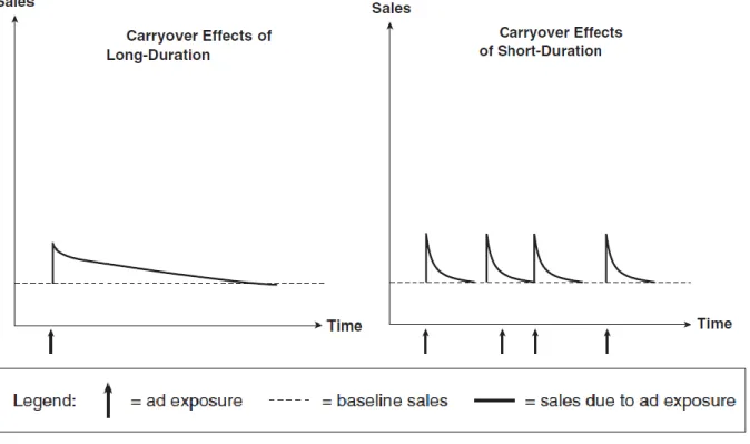
20 be seen in the figure below. The long duration that researchers often find is due to the use of data with long intervals that are temporally aggregate. Consequently, data should be used as disaggregate as possible (Clarke, 1976; Tellis, 2006).

Figure 4 – Carryover effect of advertising (Tellis, 2006)

To incorporate the carryover or lag effect into our models, the third set of models was developed (Model 3) that considers the investments in media and target variables over several days.

Specifically, three subtypes of this model were built based on:

a) Unique days - models with investments from X unique days before. They consider only 1 day before, and not a sum of days.

b) Sum of days - Models with investments from the sum of X days before, considering today’s investment.

c) Digital one day before than offline - models with investments of Digital one day before than offline.

Also, each subtype can be broken down into two sets of models. The first considers the digital investment as only one media channel (Model31) whereas the second breaks down investment in digital media by channel (Model32), resembling Model 1 and Model 2 built initially.

Below you can find an example of each subtype of the Model 3:

a) model32_Participations_1: independent variables are the investment in digital media by channel (Facebook, Google Search, YouTube, Display) and offline investment 1 day before the values of our dependent variable, which in this case is Participations.

21 b) model31_ Participations_012345: independent variables are the sum of investment in digital

and offline channels today and in the last 5 days, whereas the dependent variable is the value of Participations today.

This third set of models required specific data preparation in excel to create the variables with the lag effects desired for each model.

Even though that the models with the best accuracy metrics registered an Adjusted R-squared over 80%, by plotting the residuals during a certain period of the promotion, the models could not explain a sudden increase in the number of Participations. Therefore, by investigating why there was a rise in the number of Participations that the models were not able to account for.

Also, since Sunday was a day with different behavior than the other days, we analyzed if there was any statistically significant change in Participations by day of the week, which could be further used to improve the accuracy of the models. To do that, it was added to the models with best Adjusted R-Squared, the days of the week as dummy independent variables. The baseline was Sunday so that it could be measured the change in the target variable of Participations on each day, relative to Sunday.

22

4. IMPLICATIONS AND DISCUSSION

4.1.

L

R

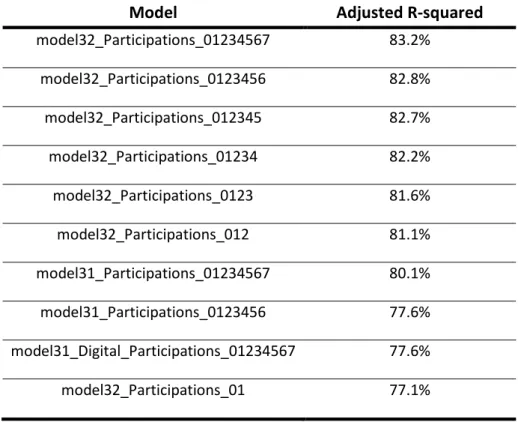
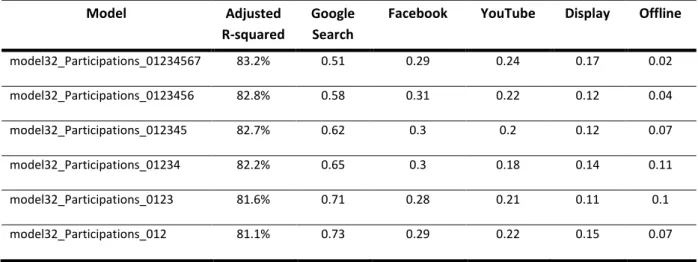
Some insights can be uncovered from the models with the highest Adjusted R-squared. This is a measure that indicates the percentage of the variance in the target variable that the independent variables explain collectively. Adjusted R-squared is preferred over the R-squared because the latter never decreases when a regressor is added to the model, regardless of the contribution of that new variable. Conversely, the Adjusted R-Squared penalizes the model when unnecessary variables are added, which is useful to prevent overfitting and compare candidate models with a different number of independent variables (Montgomery et al., 2012).

Model

Adjusted R-squared

model32_Participations_01234567 83.2% model32_Participations_0123456 82.8% model32_Participations_012345 82.7% model32_Participations_01234 82.2% model32_Participations_0123 81.6% model32_Participations_012 81.1% model31_Participations_01234567 80.1% model31_Participations_0123456 77.6% model31_Digital_Participations_01234567 77.6% model32_Participations_01 77.1%

Table 1 - Models with the highest adjusted r-squared

The first insight we can glean from this table is that Participations is the dependent variable in all models. This means that several media mixed explained better the variance of this target variable, which is positive for the “company” since this target variable is the best proxy for sales.

The second insight is that the subtype Model 32 b), which represents the sum of offline and digital investment by channel over several days, is present in most of the models with the highest Adjusted R-squared. This means that when the investment over several days by media channel is considered, the models can better predict the variance in Participations, and as a result, sales. This result is aligned with the carryover or lag effect of advertising mentioned in section 2.3.1. Evolution, which represents the effect of advertising that continues in the periods after the ad impacted a user (Tellis, 2006). Also, the fact that the accuracy of the models is higher when online media is divided by channels, enables the optimization of media budget by channel.

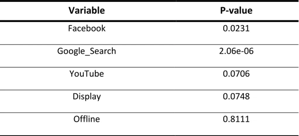
23 The p-values of the models with the highest Adjusted R-squared were similar. As an example, we will analyze the model with the highest Adjusted R-Squared:

Variable

P-value

Table 2 - P-values of the model32_Participations_01234567

The first thing that stands out from this table is that Google Search is the variable that has, by far, the lowest p-value. Hence, paid search is the channel that can explain more of the variance in

Participations. This finding is aligned with the fact that 59.4% of the Signups were attributed to paid search.

Another relevant data point is the very high p-value of the Offline variable, meaning that, according to this model, the offline channel did not make a statistically significant contribution towards the variance in Participations.

Considering a standard p-value of 0.05, besides Google Search, Facebook is also statistically

significant, suggesting that investing in this channel is associated with changes in Participations. On the other hand, the p-values from Display and YouTube channels are not statistically significant. The efficacy of each channel cannot be attached solely to the p-values of the model. These results are influenced by the funnel effects and ad targeting biases, described in section 2.3.3.2. Challenge 2:

Selection Bias, exacerbated due to the use of the last-touch attribution model on the campaign.

Thus, the literature review supports and helps to interpret the p-values on the table above.

Concretely, as per section 2.4. Attribution, one of the limitations of last-touch methodologies is that it does not consider vital interactions along the customer journey, unfairly rewarding lower funnel channels (Nisar & Yeung, 2018), which consequently tends to skew media investment away from higher-funnel channels (Interactive Advertising Bureau, 2017). Online advertising impacts particularly the later funnel stages, whereas classic advertising remains a necessity to build brand strength or to convey a brand’s positioning toward a broad audience (Pfeiffer & Zinnbauer, 2010). In this campaign, Television was used to reach the Brazilian population through a renowned Sunday night show. On the other hand, digital media was used to drive people to signup and eventually participate. Hence, in this campaign, the use of the last-touch attribution model unfairly rewarded the lower-funnel channels, which are the digital ones, potentially skewing media investment away from higher funnel channels, in this case Television, penalizing its explanatory power of the dependent variable.

Additionally, to further undermine the p-value of Television, we must remember that the dependent variable is Participations, which can only happen through digital media touchpoints.

24 Within the digital channels, paid search is the one at the end of the funnel i.e., closer to the moment of participation, because users that have already decided they wanted to sign up, typed into Google’s search engine a query related to the promotion, clicked on the ad, signed up and participated. To get a more accurate measurement of the contribution of each channel toward the final conversion, marketers should rely on Multi-touch Attribution Models.

Moreover, solutions to correct for the paid search bias on marketing mix models have been suggested by academic research. The first, proposed by (Chen et al., 2018) uses causal diagrams of the search ad environment to derive a statistically principled method for bias correction based on the back-door criterion. The second, suggested by (Chan & Perry, 2017) utilizes the search volumes for relevant queries as a control variable for the component of underlying demand from users likely to perform product-related searches. None of these approaches was feasible because the search query data necessary to improve the models were not available.

Afterward, the coefficients of the models with the highest Adjusted R-squared were analyzed:

Model Adjusted

R-squared

Google Search

Facebook YouTube Display Offline

model32_Participations_01234567 83.2% 0.51 0.29 0.24 0.17 0.02 model32_Participations_0123456 82.8% 0.58 0.31 0.22 0.12 0.04 model32_Participations_012345 82.7% 0.62 0.3 0.2 0.12 0.07 model32_Participations_01234 82.2% 0.65 0.3 0.18 0.14 0.11 model32_Participations_0123 81.6% 0.71 0.28 0.21 0.11 0.1 model32_Participations_012 81.1% 0.73 0.29 0.22 0.15 0.07

Table 3 - Coefficients of the models with the highest adjusted r-squared From this table, one can highlight that when the models consider a lower number of days, the coefficient of Google Search is also lower. This finding makes sense since paid search is the channel at the end of the conversion funnel, having almost an immediate effect on the target variable Participations.

25

4.2.

R

One of the main assumptions of Ordinary Least Squares regressions is homoscedasticity or

homogeneity of variance, which is satisfied if the residuals have constant variance, regardless of the value of the dependent variable. If the opposite happens, we are in the presence of

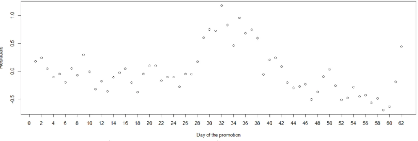
heteroscedasticity. To verify this assumption is common to plot the residuals, and see whether there are patterns i.e. if they are random and uniform (Elliot & Tranmer, 2008). When plotting the residuals of the model with the highest Adjusted R-squared, we observe that the model could not explain the variability during the period between day 29 and 38.

Figure 5 - Residuals of the model with the highest adjusted r-squared

To check for heteroscedasticity with an algorithmic approach, the Breusch-Pagan test was used (Breusch & Pagan, 1980). In this case, the p-value equals 0.5005, so the null hypothesis of homoscedasticity would not be rejected.

Additionally, to check for the presence of autocorrelation in the residuals of standard least-squares models, the Durbin-Watson test was performed (Watson & Durbin, 1950, 1951). The p-value of the test was 2.2e-16, so the null hypothesis that there is no correlation among residuals is rejected. Also, we observe that the DW statistic is 0.30437, indicating that successive error terms are positively correlated.

We named this period between days 29 and 38 the “period T” to understand the gap in media allocation per channel and Participations between this period T and the other days of the promotion, except this period.

While investigating any external cause for this situation, it was found that day 33, a Saturday, was the date of the first draft, when the first big prize was randomly given to participants. Therefore, our model could not accurately predict Participations during period T. On the days before that draft, Participations rose because people wanted to be eligible to win the first big prize. After that day, the social proof utilized in media messages from the first winner explains the boost in Participations, which our model does not.

On day 32, the day before the first draft, Participations hit an all-time high even though investment in media did not increase accordingly. This day is the highest point in the plot of the residuals, meaning, is the day where the model could not explain more of the variability in Participations. Besides people