HOW DOES PAST FORECAST BEHAVIOR AFFECT ANALYSTS’ EMPLOYMENT OUTCOME?
Maria João de Almeida Marcelino 152412024
Abstract
Supervisor Professor José Faias
Dissertation submitted in partial fulfillment of requirements for the degree of International Master of Science in Finance, at Universidade Católica Portuguesa, January 2015.
We study the relationship of sell-side analysts’ performance and their employment outcomes in the U.S. from 1983 to 2013. Analysts with a weak accuracy score are more likely to leave the job and less likely to experience a job-upgrade. Controlling for accuracy and experience, bolder and younger analysts are also more likely to experience job-termination. Additionally an Institutional Investors’ all-star has a lower chance of job-termination in case of a weak performance. Finally from 2003 onwards, after Wall Street’s regulation enforcement, employment outcome becomes less sensitive to an analyst’s past performance.
i
Acknowledgements
I would like to thank everyone who contributed in some way to my work in this thesis and followed me in my two year-experience in Católica.
Foremost, I would like to express my sincere gratitude to my supervisor Professor José Faias for his support, patience and availability in guiding my thesis. His knowledge and skill added considerably to my Master experience.
I thank all my Master fellows for the days and nights we were working together, and for all the fun we somehow still managed to have in the last two years.
I must acknowledge Sara for always pushing me to work harder and Marta for bringing kindness to a new level.
João, thanks for always providing me with a different perspective and for your disposition to teach me so much.
A special thank goes out to Isabel for her fellowship and for keeping me balanced. We make a great team.
To my dearest friends, Roger, Rita, Rita Mª, Pedro, Mª Rita, Mariana, Margarida and Lara, thank you for your friendship, advice and support during these two vivid years (and many more). I would also like to thank the ‘Fundação para a Ciência e a Tecnologia’ for financial and data support.
My thanks also go to my big cousins, Sofia, Carla and Vitor, for discussing several thesis-related topics with me and for listening to my outbursts. Tia Lúcia, Cris and Albina, thank you for being always here for me.
Finally, a huge thank you to my everythings: to my Mum for being my safe haven; to my Dad for being my guidance; and to my sister Lilita for being my better half. I thank you for the unconditional love, unyielding support and for always believing in me, especially in this project of mine.
ii Table of Contents I. Introduction...1 II. Data...5 III. Methodology...7 IV. Results...14 VI. Conclusion...29 References...32
iii
Index of Figures
Figure I – Features of Investment Banks over Time………..……….10 Figure II – Forecast Performance and Job-Termination………..…………15
Index of Tables
Table I - Forecast Accuracy and the Likelihood of Employment Outcome…………....18 Table II - Forecast Accuracy, Experience and the Likelihood of Employment Outcome…….……….…….21 Table III - Forecast Audacity, Experience and the Likelihood of Employment Outcome...23 Table IV - Forecast Performance, All-Stars and the Likelihood of Job-Termination...26 Table V - Forecast Performance, Sub-Periods and the Likelihood of Employment Outcome…..……….……….…...……….…...…28
1
I. Introduction
In the U.S., investment banks spend a great amount of money annually on equity research (e.g., Francis et al. (2004)), the latter used by investors to help making investment decisions (e.g., Madan et al. (2003)) and by firms to market their securities (e.g., Krigman et al. (2001)). In this sense, sell-side financial analysts have long been an important topic among academic researchers due to their key role in capital markets.1
Following Hong et al. (2000) we examine the impact of an analyst’s past performance and her employment outcome (e.g., Clement and Tse (2003)) for a sample of U.S. analysts from 1983 to 2013. We build sell-side analysts’ rankings for their accuracy and audacity levels, proxies for forecast performance, and set measures to define three possible career outcomes: job-termination, job-upgrade and job-downgrade. Overall, we find that forecast performance impacts an analyst’s likelihood of job-termination more than being upgraded to a high-status bank. Our results come in line with previous literature that i) identify a positive relation between forecasting accuracy and promising career outcome (Clement (1999)); ii) consider that analysts producing bold forecasts, i.e. incur in ‘anti-herding’ behavior have a higher chance to experience job-termination (Hong et al. (2000)). Nevertheless, despite the statistical significance of the results, we find a decrease in the magnitude of the impact of analysts’ performance on their employment outcome. In accordance, we find that inaccurate and bold performers are less likely to leave the sample if they produce forecasts after the year of 2003, namely after the implementation of the SEC regulations. Finally, and in line with previous literature, an analyst belonging to the group of all-stars has a lower chance of job-termination (Leone and Wu (2007)).
1
When searching on the Social Science Research Network (SSRN) eLibrary we obtain 2,245 results for papers in which the word “analyst” appears in the abstract, of which in 1,003 the combination of the words “analyst and earnings” is to be found.
2 Early research on sell-side analysts focused on the statistical properties of earnings forecasts (O’Brien (1988)) and its investment value (e.g., Womack (1996)). More recently, the impact of analyst forecasts behavior has become a topic of interest (e.g. Agrawal et al. (2006)). For instance, previous research studies the relation between the trading volume achieved by an investment bank and its analysts’ forecasting ability, or how a sell-side analyst’s performance influences analysts’ labor market concerns (e.g., Alford and Berger (1999), and Irvine (2004)).
In addition, when assessing analysts’ performance, the consensus is that precision (i.e. accuracy) in forecasting is relevant (e.g., Gu and Wu (2003)). Analysts that are more precise, shift prices readily (e.g., Jackson (2005)), are acknowledged and compensated for their work (e.g., Stickel (1992)) and have greater chances of experiencing job-upgrade (e.g., Hong and Kubik (2003)). Mikhail et al. (1999) observe that analyst forecast accuracy is related with job change, indicating an association with remuneration. Though remuneration is not directly observed in I/B/E/S, we consider the relation between career outcomes and analysts’ job change across investment firms during our period of analysis (e.g., Holmstrom (1999)).
First, we examine the impact of forecast accuracy on employment outcome. The labor market identifies an agent’s past accuracy as a key indicator of her ability. Thus analysts’ career prospects (i.e. job-termination or job-upgrade) rely upon this evaluation of ability and are subsequently related to an analyst’s past action. In line with Hong et al. (2000) we confirm that less accurate analysts have a higher chance of experiencing job-termination and a lower chance of being upgraded.
Previous research also finds that forecast audacity (i.e. boldness) is an indicator of an analyst’s herding behavior and ability (e.g., Scharfstein and Stein (1990)). Clement and Tse (2005) observe a greater accuracy for bolder analysts; and Bernhardt et al.
3 (2006) report results on analysts’ propensity to “anti-herding”. Other studies identify an analyst’s incentive to herd toward the consensus, either because the consensus is a good aggregator of private information (e.g., Jegadeesh and Kim (2009), and Welch (2000)), or because the analyst does not want to deviate from the norm (e.g., Hong et al. (2000)).
When controlling for accuracy, we observe that analysts issuing bold forecasts have a higher likelihood of experiencing job-termination compared to analysts that herd. However, if an analyst is bold and experienced she is less likely to stop producing forecasts than young analysts. Our findings, despite in a smaller magnitude, are in line with previous literature that finds that an analyst incurring in a herding behavior has a higher chance of keeping her job and that experience influences an analyst’s incentives (Hong et al. (2000)). Interestingly, Clement and Tse (2005) find that forecasting audacity is an indicative of an analyst holding more private information, thus delivering greater reports to the buy-side of the market. Moreover, investment firms value analysts with a bold attitude when forecasting stocks, because it leads to a promotion of the stock, and consequently brings more money to the brokerage house the analyst works for (Michaely and Womack (1999)). Accordingly, we expected bold analysts to be less likely to leave the sample than herding analysts. However our results suggest a slight tendency for the opposite to happen, only when controlling for experience is forecasting audacity an asset.
Furthermore we study the ‘all-stars’, i.e., the financial analysts ranked in the Institutional Investor magazine annual surveys from 1997 to 2013. The Institutional Investor’s rankings of financial analysts are considered a measure of analyst reputation (Krigman et al. (2001), and Cliff and Denis (2004)). Previous research demontrates that these rankings have a meaningful role in identifying high-status analysts in the labor market (Leone and Wu (2007)) and in determining analysts’ career concerns (e.g.
4 Stickel, 1992). Thus, we expect all-stars to have a greater career outcome than regular sell-side analysts. In the early 21st century Hong and Kubik (2003) study the likelihood of job-downgrade for all-stars. Their most relevant findings are that a weak forecasting accuracy has a minor impact on the likelihood of job-downgrade for all-stars. We analyze the likelihood of job-termination on our I/B/E/S analysts including a subsample of all-stars. Despite the different career outcome, since our dependent variable is an analyst experiencing job-termination, we too observe that all-stars’ career concerns, i.e. likelihood of job-termination is less sensitive to past forecast performance.
Finally, our period of study covers the enforcement of several settlements on the Wall Street capital market. For instance, on October, 2000, the U.S. Securities and Exchange Commission (SEC) agreed on a set of ‘fair disclosure’ rules; on April, 2003, the SEC, NASD, NYSE, and the top U.S. largest investment firms accorded to an enforcement agreement to address issues of conflict of interest within their businesses. These rules intend to stop the act of selective disclosure, whereby firms give Wall Street analysts and large shareholders information in advance (e.g., Agrawal et al. (2006), Cohen et al. (2010)).2 Previous literature has focused on the impact of the new regulation on sell-side analysts’ decision-making, company coverages and forecast production, due to the change in the information flow on Wall Street (Jorion et al. (2005)). Thus, it is likely that as analyst performance is influenced by the disclosure rules, an analyst’s career outcome is indirectly impacted. In this sense, we break our analysis in sub-periods and examine the relationship between forecast performance and employment outcome (i.e. job-termination and job-upgrade) before and after the implementation of the SEC regulations. We find evidence of a declining importance of an analyst’s forecasting accuracy and audacity regarding job-termination. After the year
2
The analyst regulations, issued between 2000 and 2003, include Regulation Fair Disclosure (Reg FD), NASD Rule 2711, NYSE Rule 472, and Regulation Analyst Certification (Reg AC), culminating in the Global Settlement of 2003 (Barniv et al. (2009)).
5 of 2003 less accurate and bolder analysts are less likely to experience job-termination compared with the earliest period. In addition, we observe a growing importance of forecast audacity regarding job-upgrade for the period after the implementation of the regulations.
The remainder of the dissertation proceeds as follows. In Section II, we describe the data. In Section III we construct the measures for employment outcome and forecast behaviors, reputation and bias. Section IV presents our empirical results. In Section V we conclude.
II. Data
We export from I/B/E/S Detail History File analysts’ earnings forecasts of U.S. firms between 1983 and 2013. We observe forecasts of roughly 18,500 sell-side individual analysts, employed in about 850 investment banks and covering 17,600 firms. The I/B/E/S Detail History File assigns an exclusive numerical code to all individual security analysts and investment firms. We use these codes to track both earnings forecasts and job-background of the analysts in I/B/E/S.
Every year in October the Institutional Investor, a U.S. finance magazine, releases a ranking (i.e. first, second, third and runner-ups) indicating the U.S. sell-side analysts that achieved the highest performance for the different industries and sectors in a year. These ranking reflects the voting of buy-side analysts and portfolio managers on the performance of their counterparts. Sell-side analysts are assessed on several attributes that serve as proxies for their yearly accomplishments, including accuracy and optimism bias. In order to compare this group of strong-performers with our I/B/E/S analysts we hand collected the names of the All-America Research Team analysts, also referred as all-stars, and tracked them on I/B/E/S.
6 The I/B/E/S Detail Recommendations File encompasses analyst-by-analyst recommendations for a security. Moreover, the Detail Recommendations File also provides two variables that indicate, respectively, the first initial and last name of the analysts, and the institution’s identity in the database.3
This information allows us to determine the names of the sell-side analysts that appear on the Institutional Investor’s All-America Research Team and the brokerage house they work for between 1997 and 2013. We analyze the estimates of about 2000 all-stars.
Analysts in our sample follow about 10 firms in a year, with a standard deviation of 10 firms. Across the sample we observe that analysts usually follow companies from the equivalent industry group. We use the Standard & Poor’s Global Industry Classification Standard (GICS) industry codes, supplied by COMPUTSTAT, to classify the companies on our sample. The GICS industry code categorizes companies into four different partitions: sectors, industry groups, industries and sub-industries. In our sample period we identify 51 sectors, 61 industry groups, 84 industries, and 117 sub-industries. By assigning firms to a GICS industry code, we allocate each analyst to an industry according to the firms she covers. According to Boni and Womack (2006) partition based on the GICS codes is a reasonable proxy for analysts’ specialization by industry. The GICS classifications account for stock return co-movements, cross-sectional variations in valuation-multiples, forecasted and realized growth rates, and key financial ratios better than other classification schemes Bhojraj et al. (2003). In our dataset, investment firms cover on average 3 industry groups, with a standard deviation of 4. The maximum industry groups an institution covers is 16. Analysts cover on average only 1 industry, with a standard deviation of 0.5. The maximum number of industries an analyst covers in our sample period is 5 industries.
3
Thomson Reuters no longer provides the Broker and Analyst Translation files used by previous papers (Clarke et al. (2007)) to translate broker and analyst codes to actual names.
7 Overall, we analyze the estimates of 31,982 security analysts’. On average an analyst stays in our sample for 8 years, with a standard deviation of about 5 years. Only 13 analysts remain in our database for the whole 30-year period. The 90th percentile is 15 years, and the 10th percentile is 3 years. We find that analysts leave our sample for the following reasons: 1) the analyst leaves the job; 2) the analyst changes to a company not present in I/B/E/S; 3) the analyst works for a brokerage house that stops submitting analysts’ forecasts to I/B/ES. In any case, we only consider analysts with a three-year minimum of forecast history in I/B/E/S because it better proxies for forecasting ability (Hong et al. (2000)).
With the individual analyst’s earnings forecasts gathered from I/B/E/S, we are able to construct the key variables to examine analyst's performance. We assess an analyst’s career evolution by creating the necessary indicators of job changes and job-termination. Secondly we construct measures of their performance based on the produced earnings forecasts, since past performance is considered a determinant of an analyst’s career outcome. Hence, in the following section we discuss how to construct the forecast accuracy and audacity measures for each analyst, proxies for analysts’ precision and bias, respectively; and how we identify analysts’ job-termination, upgrades or downgrades.
III. Methodology
In this section we present the dimensions for employment outcome, forecast accuracy and audacity.
A. Measures of Employment Outcome
We first construct proxies for analysts’ career outcomes. Over the period security analysts produce and submit forecasts to the I/B/E/S, however this database does not
8 provide each analyst’s individual career path throughout their activity. To determine whether the analyst has left her job, has been upgraded or downgraded we track in the database if an analyst stops producing earnings forecasts or changes to a different brokerage house.
A.1. Job-Termination
Our sample of analysts only comprises sell-side analysts. Most security analysts in the U.S. produce earnings forecasts and submit their forecasts to I/B/E/S (e.g., Peterson and Peterson (1995), and Hong et al. (2000)). Generally, sell-side analysts strive to be part of the Institutional Investors All-American Research Team (e.g., Leone and Wu (2007), and Boris et al. (2011)), while buy-side analysts’ aspiration is to become a mutual fund manager. Thus, it is unlikely that a sell-side analyst will leave her job to obtain a new job on the buy side (e.g, Stickel (1992), and Nocera (1997)). Hereafter, we assume an analyst producing forecasts in year 𝑡, yet no longer producing forecasts to
I/B/E/S in year 𝑡 + 1, is considered to experience job-termination in year 𝑡 + 1. The number of analysts leaving jobs per year is around 345. If we consider two different periods, before and after 2003, we obtain an average of 333 analysts leaving the sample from 1985 to 2003; thereafter the number of analysts leaving the sample per year is on average 373 analysts.
A.2. Upgrade & Downgrade
We consider the changes of the analysts between investment firms to define other possible career outcomes besides job-termination. By looking at the features of the investment firms the analyst is working on, before and after changing job, we determine whether an analyst experiences job-downgrade or job-upgrade. We assume that the most prominent investment firms have a higher number and more diversified base of clients compared to other investment firms. Hence, high-status investment firms employ more
9 analysts to cover all sectors and respective firms. In contrast, small investment firms naturally employ fewer analysts, since these tend to only represent regional companies or focus on a particular sector, having therefore a targeted and reduced set of clients.
The proxy for the number of analysts employed by a brokerage house per year is the number of analysts on I/B/E/S producing forecasts for each individual investment bank. We consider that an analyst is upgraded (downgraded) in case she serves an investment bank in year 𝑡 employing less (more) than 25 analysts and changes in year 𝑡 + 1 to an investment bank with a minimum (a maximum) of 25 analysts. Depending on the status of the investment bank in which the analyst works, we have two employment outcome dimensions. An analyst’s upgrade when she moves from a low-status bank to a high-low-status bank and downgrade if the opposite situation is to observe.
In this 30-year period on average an investment bank enlists around 18 analysts. If we divide our sample in two periods, we observe in the first half of our sample a mean of 19 analysts per institution, as in our most recent sub-period, on average, 17 analysts work for a brokerage house. In addition, an investment bank at the bottom 20% of the distribution has around 3 analysts in activity, whereas a bank at the 80th and 90th percentiles employs on average 23 and 42 analysts, respectively. Thus, we consider the cut-off of 25 analysts an acceptable number to represent the proxy for high-status companies over our period of analysis. In Figure I we present further descriptive statistics of the features of the brokerages and the number of analysts that works for the latter.
Finally, for the period between 1985 and 2013, on average, per year, 29 analysts are downgraded, while 33 analysts are upgraded. If we divide our sample in two subperiods, i.e., after and before the year of 2003, we observe a slight change in these numbers. Before 2003 the average downgrades per year affects around 27 security
10 analysts while, after 2003 the downgrades increase to a 35.5-average per year. In respect to upgrades, the average per year increases from about 28 to roughly 38 analysts in the second half of our period of study.
Figure I
Features of Investment Banks over Time
Panel A presents the number of investment banks in I/B/E/S from 1983 to 2013. Panel B presents the values for the average, median, 25th and 75th percentiles of the sell-side analysts working for the investment banks in I/B/E/S from 1983 to 2013. The cut-off value in Panel B is 25 and is indicative of our definition for a high-status bank. An investment bank employing more than 25 analysts in a given year is considered a high-status bank.
Panel A: Brokerage Houses in I/B/E/S from 1983 to 2013
Panel B: Analysts working for a Brokerage House in I/B/E/S from 1983 to 2013
B. Measures of Performance
We consider the earnings forecasts from I/B/E/S Detail File to measure analyst performance along two main dimensions that reflect both analyst reputation and bias:
0 100 200 300 400 500 1 9 8 3 1 9 8 4 1 9 8 5 1 9 8 6 1 9 8 7 1 9 8 8 1 9 8 9 1 9 9 0 1 9 9 1 1 9 9 2 1 9 9 3 1 9 9 4 1 9 9 5 1 9 9 6 1 9 9 7 1 9 9 8 1 9 9 9 2 0 0 0 2 0 0 1 2 0 0 2 2 0 0 3 2 0 0 4 2 0 0 5 2 0 0 6 2 0 0 7 2 0 0 8 2 0 0 9 2 0 1 0 2 0 1 1 2 0 1 2 2 0 1 3
Number of Brokerage Houses
0 10 20 30 40 1 9 8 3 1 9 8 4 1 9 8 5 1 9 8 6 1 9 8 7 1 9 8 8 1 9 8 9 1 9 9 0 1 9 9 1 1 9 9 2 1 9 9 3 1 9 9 4 1 9 9 5 1 9 9 6 1 9 9 7 1 9 9 8 1 9 9 9 2 0 0 0 2 0 0 1 2 0 0 2 2 0 0 3 2 0 0 4 2 0 0 5 2 0 0 6 2 0 0 7 2 0 0 8 2 0 0 9 2 0 1 0 2 0 1 1 2 0 1 2 2 0 1 3
11 The earnings forecast accuracy as a proxy for analyst reputation; the earnings forecast audacity as a proxy for bias.
Analyst reputation and bias are company and industry dependent. Thus, if in a given year, we confront an analyst’s average forecast error to the one of all the other analysts in the sample we may obtain inaccurate results, because the predictability of earnings for some companies, depending on the industry or on the coverage invested, is easier than others. Following Hong et al. (2000), we use a scoring methodology to construct annual performance scores.
B.1. Forecast accuracy
We build a yearly performance ranking with basis on analysts’ forecast accuracy in order to observe individual analyst’s precision over the companies she follows. There are several alternative measures of sell-side analysts’ performance. We define 𝐹𝑖,𝑗,𝑡 as the most updated earnings per share forecast produced by analyst 𝑖 on company 𝑗 for year 𝑡; and 𝐴𝑗,𝑡 as the realized earnings per share of the same firm 𝑗. We consider the absolute variation between the forecasted and the realized earnings per share our measure of analysts’ forecast accuracy for company 𝑗 in year 𝑡:
𝑓𝑜𝑟𝑒𝑐𝑎𝑠𝑡 𝑎𝑐𝑐𝑢𝑟𝑎𝑐𝑦 𝑒𝑟𝑟𝑜𝑟 = |𝐹𝑖,𝑗,𝑡− 𝐴𝑗,𝑡| (1) On average, an analyst examines more than one company in a given year. Thus, we collect, for each company she follows in a year, the forecasting accuracy error. Thereafter, an option would be to compare the average forecast accuracy error of the analysts producing earnings forecasts in the same year. However, most analysts focus on distinct companies, distinct business sectors and not all companies are equally easy to predict. Instead, based on the forecast accuracy errors we sort the analysts by company 𝑗 and assign a rank based on the error. The analyst with the smallest forecast accuracy error is the most accurate analyst, thus receiving a rank of one. If there is a tie,
12 meaning that two or more analysts have the same accuracy level, we appoint to the analysts the mean value of their position in the ranking. According to this system, independently of the forecast accuracy errors analysts achieve for different firms, the analyst yielding the most precise forecast for company X has the same accuracy rank as the analyst yielding the most precise forecast of company Y.
We could assume that an analyst averaging lower ranking scores (e.g. 1 or 2 out of 56) across the companies she follows is a greater forecaster. Nevertheless, this average score might be unsuitable, since the position in the rank an analyst gets for company j is dependent on the amount of analysts producing forecasts for the same company j. If a company is thinly covered, regardless of the forecast accuracy error value, analysts covering that company have a higher chance of a low ranking position compared to analysts producing forecasts for companies with high coverage. Therefore, the ultimate score an analyst gets for a company she covers relies on the total analysts covering the company. Hence, we scale the analyst’s ranking position by the number of analysts with focus on the same company. The equation of the overall score adapting for the differences in coverage is
𝑠𝑐𝑜𝑟𝑒 = 100 − [ 𝑟𝑎𝑛𝑘𝑖,𝑗,𝑡−1
𝑛𝑢𝑚𝑏𝑒𝑟 𝑜𝑓 𝑎𝑛𝑎𝑙𝑦𝑠𝑡𝑠𝑗,𝑡−1] × 100. (2)
The 𝑛𝑢𝑚𝑏𝑒𝑟 𝑜𝑓 𝑎𝑛𝑎𝑙𝑦𝑠𝑡𝑠𝑗,𝑡 is the total amount of analysts following and producing forecasts of company 𝑗 in year 𝑡. Before computing this score, we define the criteria that at least four analysts mu cover a company 𝑗 for it to be considered in our study. The scores go from zero, for the least accurate analyst, to one hundred, for the analyst with the rank of one.
After calculating analysts’ scores for all the companies, we estimate a final score to consider as proxy for an analyst's forecast accuracy. To simply consider the mean of the analyst's scores in a year is a noisy measure for those who cover few companies in a
13 given year. Thus, our final measure of forecast accuracy is the mean of an analyst’s accuracy score in year 𝑡, 𝑡 − 1 and 𝑡 − 2. Thus, the analyst has to submit forecasts to
I/B/E/S for at least three year, for the forecast accuracy dimension to be estimated. The
highest the overall score the better the analyst’s forecast accuracy. This is a reasonable measure for estimating performance and reputation; however we need to be aware of its limitations. Some analysts, independently of the accuracy, have a higher chance of extreme mean scores. For instance, one strong or weak forecast decision on a company largely affects an analyst’s average score if she covers a small number of companies over the period considered. Likewise, analysts producing forecasts of thinly followed companies more easily get a score close to the top or bottom of the ranking, because these companies are covered by few analysts.
B.2.Measure of Forecast Audacity
The evidence of herding is based on comparing analysts’ forecasts to the consensus, with movements toward the consensus labeled as herding and movements away from the consensus labeled as audacity (i.e. bold decisions). To build the measure of the analyst's forecast audacity, we consider an identical method to our previously computed accuracy indicator. We first compute the average forecast of the analysts, except analyst 𝑖, following security 𝑗 in year 𝑡 as
𝐹̅−𝑖,𝑗,𝑡=1
𝑛∑𝑚∈−𝑖𝐹𝑚,𝑗,𝑡 (3)
In the above equation −𝑖 is the sample of all analysts, with the exception of analyst 𝑖, estimating forecasts for company 𝑗 in year 𝑡, and 𝑛 is the total number of analysts in – 𝑖. Thus, the forecast audacity error is the absolute variation of an analyst’s 𝑖 earnings forecast and all the other analysts’ averaged forecasts of the same company 𝑗 in year 𝑡:
14 We replicate the ranking methodology used in the previous subsection: We rank the analysts following a company 𝑗 in a given year 𝑡 depending on their forecast audacity errors. The bolder the analyst is, the greater (in absolute value) her earnings forecasts, meaning she deviates more from the average forecasts. We then compute the forecast audacity score as in Equation (2). The score is zero for the analyst producing forecasts for a company closer to the consensus value, and one hundred for the analyst that deviates the most from the average forecasts, i.e. produces the most biased forecasts. We finally compute for the analyst her overall audacity score, as the mean of the analyst's audacity scores in years 𝑡, 𝑡 − 1 and 𝑡 − 2. This procedure is an acceptable method that proxies for bias, yet the same cautions arise in computing this dimension as in the forecast accuracy measure.
IV. Results
With our dimensions of employment outcome and forecast performance, we now observe the impact of past forecast behavior on an analyst’s career outcome.
A. Relationship between employment outcome and forecast behavior
Starting in the early nineties, the growing notoriety of security analysts on the financial markets has called for the financial press and regulators attention mostly regarding analysts’ career concerns. For instance, analysts are indicted of releasing favorable coverages (e.g., Schroeder and Smith (2002)) and compromising the precision of their predictions (e.g., Kane (2001)) in order to comply with possible brokerage houses and companies. Contrastingly, Clarke et al. (2007) find no direct evidence that an analysts’ over-optimistic behavior is due to affiliations between financial institutions. Moreover, Brown et al. (2013) find that issuing forecasts below the average leads to an increase of analysts’ credibility among clients, and not a change in their compensation.
15 Figure II
Forecast Performance and Job-Termination
Panel A presents the yearly average, the 5th and the 95th percentiles of the forecast accuracy and audacity scores from 1986 to 2013. The sample comprises analysts with a minimum of three-years of experience in producing forecasts to I/B/E/S. The scores are computed as the mean of each analyst’s score in years 𝑡, 𝑡 − 1 and 𝑡 − 2. A score close to zero indicates an analyst’s weak performance; a score close to one hundred reveals the most accurate and bold forecasters in our sample. Panel B presents the yearly percentage of security analysts in I/B/E/S that experience job-termination from 1986 to 2013; and the period averaged percentage of analysts experiencing job-termination. An analyst is considered to be leaving her job if she is in I/B/E/S in a given year, and is no longer in I/B/E/S in the next year.
Panel A: Evolution of the forecast performance scores from 1986 to 2013
Panel B: Evolution of I/B/E/S analysts’ job-terminations from 1986 to 2013
In Figure II we present some descriptive statistics for the performance measures and job-termination of our sample of analysts. Panel A presents the average value and the top and bottom percentiles for the forecast accuracy and audacity measures. We observe that for the period between 1985 and 2013 the average performance scores
30 40 50 60 70 1 9 8 6 1 9 8 7 1 9 8 8 1 9 8 9 1 9 9 0 1 9 9 1 1 9 9 2 1 9 9 3 1 9 9 4 1 9 9 5 1 9 9 6 1 9 9 7 1 9 9 8 1 9 9 9 2 0 0 0 2 0 0 1 2 0 0 2 2 0 0 3 2 0 0 4 2 0 0 5 2 0 0 6 2 0 0 7 2 0 0 8 2 0 0 9 2 0 1 0 2 0 1 1 2 0 1 2 2 0 1 3
5th Per. Accuracy Average Accuracy 95th Per. Accuracy
5th Per. Audacity Average Audacity 95th Per. Audacity
0% 5% 10% 15% 20% 25% 1 9 8 6 1 9 8 7 1 9 8 8 1 9 8 9 1 9 9 0 1 9 9 1 1 9 9 2 1 9 9 3 1 9 9 4 1 9 9 5 1 9 9 6 1 9 9 7 1 9 9 8 1 9 9 9 2 0 0 0 2 0 0 1 2 0 0 2 2 0 0 3 2 0 0 4 2 0 0 5 2 0 0 6 2 0 0 7 2 0 0 8 2 0 0 9 2 0 1 0 2 0 1 1 2 0 1 2 2 0 1 3
16 remain relatively steady. For our sample period, the mean for the forecast accuracy performance is 50.12 (analysts’ scores range between 0 and 100) with a standard deviation of about 8 points. The score values for the 25th and 75th percentiles of the accuracy score are 38.21 and 62.50, respectively. For the forecast audacity score the mean value is 49.68, standard deviation around 9, while the 25th percentile takes the score value of 35.71, and finally the 63.82 is the score that indicates the 75th percentile of the audacity score. The sum of the analysts no longer producing forecasts in year 𝑡 + 1 divided by the total analysts submitting forecasts in year 𝑡 indicates the likelihood of job-termination. We compute the likelihood of job-upgrade (downgrade) by dividing the number of analysts working for a brokerage with fewer (more) than 25 analysts in year 𝑡 that changed to a brokerage with more (fewer) than 25 analysts in year 𝑡 + 1 by the total number of analysts producing forecasts in year 𝑡 and 𝑡 + 1. Panel B presents the percentage of analysts that stopped producing forecasts throughout our period of analysis. We observe that the percentage of analysts experiencing job-termination does not follow a constant path, for instance in the year of 1997 only 2% of the analysts in our sample stopped producing forecasts as in 2003 almost 20% of the analysts experienced job-termination. Averaging across our sample period, the likelihood of an analyst leaving the job is 10.6%. Additionally, the likelihood of an analyst in our sample being upgraded is about 1.6%, and the probability of being downgraded is 1%.
17
B. Employment outcome and forecast accuracy
Next we present the regression that relates employment outcome with forecast accuracy: 𝑒𝑚𝑝𝑙𝑜𝑦𝑚𝑒𝑛𝑡 𝑜𝑢𝑡𝑐𝑜𝑚𝑒𝑖,𝑡+1= = 𝛼 + 𝛽1𝑓𝑜𝑟𝑒𝑐𝑎𝑠𝑡 𝑎𝑐𝑐𝑢𝑟𝑎𝑐𝑦𝑖,𝑡+ 𝑎𝑣𝑒𝑟𝑎𝑔𝑒 𝑐𝑜𝑣𝑒𝑟𝑎𝑔𝑒 𝑒𝑓𝑓𝑒𝑐𝑡𝑠𝑖,𝑡+ + 𝑛𝑢𝑚𝑏𝑒𝑟 𝑜𝑓 𝑓𝑖𝑟𝑚𝑠 𝑐𝑜𝑣𝑒𝑟𝑒𝑑 𝑒𝑓𝑓𝑒𝑐𝑡𝑠𝑖,𝑡+ + 𝑏𝑟𝑜𝑘𝑒𝑟𝑎𝑔𝑒 ℎ𝑜𝑢𝑠𝑒 𝑒𝑓𝑓𝑒𝑐𝑡𝑠𝑖,𝑡+ 𝑖𝑛𝑑𝑢𝑠𝑡𝑟𝑦 𝑒𝑓𝑓𝑒𝑐𝑡𝑠𝑖,𝑡+ + 𝑦𝑒𝑎𝑟 𝑒𝑓𝑓𝑒𝑐𝑡𝑠𝑡+1+ 𝜀𝑖,𝑡+1 ( (5)
where 𝑒𝑚𝑝𝑙𝑜𝑦𝑚𝑒𝑛𝑡 𝑜𝑢𝑡𝑐𝑜𝑚𝑒𝑖,𝑡+1 indicates whether analyst 𝑖 stops producing forecasts or is upgraded in year 𝑡 + 1. The 𝑓𝑜𝑟𝑒𝑐𝑎𝑠𝑡 𝑎𝑐𝑐𝑢𝑟𝑎𝑐𝑦𝑖,𝑡 indicates the analyst’s past forecast accuracy in year 𝑡; 𝛽1 sizes the impact of past forecast accuracy on the likelihood of experiencing employment outcome the next year. Since our number of job-downgrades is reduced, further on we focus only on the relationship between past forecast behaviors and, job-upgrade or job-termination.
We also include dummies in our specification to control for possible biases in the estimations, such as the type and number of companies tracked over the period of analysis. We control for the 𝑎𝑣𝑒𝑟𝑎𝑔𝑒 𝑐𝑜𝑣𝑒𝑟𝑎𝑔𝑒 𝑒𝑓𝑓𝑒𝑐𝑡𝑠𝑖,𝑡 of the companies followed by the analyst and for the number of companies the analyst follows – 𝑛𝑢𝑚𝑏𝑒𝑟 𝑜𝑓 𝑓𝑖𝑟𝑚𝑠 𝑐𝑜𝑣𝑒𝑟𝑒𝑑 𝑒𝑓𝑓𝑒𝑐𝑡𝑠𝑖,𝑡. Additionally, we also include dummies for the 𝑏𝑟𝑜𝑘𝑒𝑟𝑎𝑔𝑒 ℎ𝑜𝑢𝑠𝑒 𝑒𝑓𝑓𝑒𝑐𝑡𝑠𝑖,𝑡, 𝑖𝑛𝑑𝑢𝑠𝑡𝑟𝑦 𝑒𝑓𝑓𝑒𝑐𝑡𝑠𝑖,𝑡 and 𝑦𝑒𝑎𝑟 𝑒𝑓𝑓𝑒𝑐𝑡𝑠𝑡+1 present in our sample.
Table I reports our results for this regression. In columns (1) and (2) the employment outcome measure identifies if the analyst leaves the job. The estimate in column (1) is a dummy variable for the analysts in the 5th percentile of the accuracy score in year 𝑡. Thus, this variable sizes the likelihood of less accurate analysts leaving
18 our sample in comparison with the remainder of the sample. In column (1) the estimate suggests that less accurate analysts (5th percentile) have a probability about 1.7 percentage points higher, of leaving their job compared to their fellows in the sample. This indicator is statistically and economically significant. Averaging for our sample period, the likelihood of an analyst leaving the sample is of 10.6% (recall Figure II); being in the 5th percentile of the accuracy score increases the likelihood of leaving the sample by around 2%.
Table I
Forecast Accuracy and the Likelihood of Employment Outcome
This table presents records for the impact of analysts’ past forecast accuracy on their future employment outcome. We consider analysts’ past earnings forecasts to compute the forecast accuracy score. In columns (1) and (2) the dependent variable is job-termination - analysts stop producing forecasts to I/B/E/S in the year to follow. In columns (3) and (4) the dependent variable is job-upgrade – analysts move to a high-status brokerage in the year to follow. The regression is Equation (5). The standard errors are in parentheses. The symbols ***, **, * represent the 1%, 5% and 10% significance levels, respectively.
Forecast Accuracy Ranking Job-Termination Job-Upgrade
(1) (2) (3) (4) Accuracy (bottom 5%) .0174** .0129* -.0053 -.0072* (.0079) (.0074) (.0035) (.0037) 5th through 10th percentile .0104 -.0047* (.0071) (.0028) 10th through 25th percentile .0099 -.0040* (.0068) (.0024) 25th through 50th percentile .0073 -.0034 (.0056) (.0021) 50th through 75th percentile -.0034 -.0009 (.0049) (.0021) Observations 31,982 31,982 28,590 28,590
We introduce in column (2) new variables that indicate an analyst's position in the forecast accuracy ranking. These estimates size the probability of an analyst, in a given position of the rank, leaving the job compared to analysts who score on the top 25th percentile of the score. Once more, we observe that the analysts with a low accuracy
19 score have a higher likelihood of leaving the job. In fact, analysts in the bottom 5% of the ranking are nearly 1.3% more likely to leave the job than their most accurate counterparts. As we go up on the score distribution, our estimates decrease and lose significance, meaning that the analyst is less likely to leave the job, yet larger effects are clearer in the bottom range of the accuracy ranking.
In columns (3) and (4) we consider job-upgrade as our employment outcome measure. The coefficient in column (3) indicates the impact of a score in the 5th percentile of the forecast accuracy ranking on the possibility of job-upgrade. We observe that weak accuracy performance leads to a fall in the likelihood of job-upgrade by around 0.5%, although not statistically significant. We introduce in column (4) the variables that indicate an analyst’s position in the accuracy ranking as we do in column (2). We observe that as we go up in the accuracy score, an analyst is more likely to be upgraded, yet there is no significant variation when analyzing the middle sets of the accuracy ranking. An analyst scoring low in accuracy is nearly 1 percentage point less likely to be upgraded than her counterparts in the 75th percentile of the accuracy ranking. Our study comprises a limited sample of job-upgrades, notwithstanding we are able to observe an influence of past forecast accuracy on an analyst’s likelihood of job-upgrade.
Ultimately, even if analysts’ compensation is influenced by other factors besides forecast accuracy, in order to remain on top of the business, analysts need to be known for forecasting expertise among the buy-side, and brokerage house directors are aware of this fact when mapping their employees’ forthcoming career (e.g., Holmstrom (1999)). Our outcomes are in line with this previous career-outcome studies that prove that weak accuracy performance origins a revised appraisal of an agent's ability to forecast and the likelihood of leaving the job or simply not progress in her career.
20 Although the results indicate that more accurate forecasters are rewarded, this effect is not symmetric. The impact is larger for extremely weak-accuracy analysts.
C. Employment outcome, forecast accuracy and experience
A further conclusion of several career-outcome studies is that employment outcome is related to an agent’s experience (e.g., Mikhail et al., 1999, and Hong and Kubik, 2003)). In this sense we now control for experience.
Thus, we have no information about the number of years an analyst works in the sell-side market. We introduce a dummy variable entitled 𝑒𝑥𝑝𝑒𝑟𝑖𝑒𝑛𝑐𝑒𝑖, this is one if the analyst in a given year 𝑡 produces forecasts to I/B/E/S for a minimum of four years and zero if the analyst has three or less years of experience.4 For instance the probability of an analyst being experienced, i.e., being in our sample for more than 3 years, is about 83%. Moreover, only 3% of the analysts in our sample have more than 10 years of experience, while only 14 analysts are in the sample from 1985 to 2013.
We estimate the impact of weak accuracy on the likelihood of employment outcome for both experienced and inexperienced analysts. We add to the regression of Equation (5), the experience dummy variable and an interaction of experience and forecast accuracy.
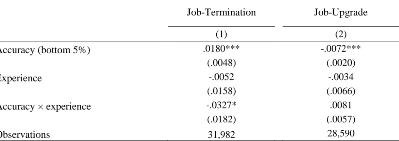
In column (1) of Table II, we consider as the dependent variable stopping the production of earning forecasts. As observed before, an analyst performing in the 5th percentile of the accuracy score has a higher chance of leaving our sample than their counterparts. An analyst in the bottom 5% of the forecast accuracy score is 1.8 percentage points more likely to leave the sample than their counterparts. Else, the coefficient of the experience variable is negative, implying that an old analyst has a lower probability of leaving her job than a younger one. Hence, this term is not
4
An analyst must be producing forecasts for at least three years for the measure of forecast accuracy to be computed.
21 statistically significant. At last, the interaction term presents a coefficient that indicates a higher likelihood for inexperienced analysts to stop producing forecasts after performing weakly compared to their older counterparts. If an analyst has a low accuracy score in a given year but is experienced, she is about 3 percentage points less likely to leave the sample than a young analyst scoring low. This coefficient is statistically significant. Thus, performing weakly greatly affects the chance of job-termination for a young analyst.
Table II
Forecast Accuracy, Experience and the Likelihood of Employment Outcome
This table presents records for the impact of analysts’ past forecast accuracy and experience on their future employment outcome. We consider analysts’ past earnings forecasts to compute the forecast accuracy score. We consider the number of years an analyst is producing forecasts to
I/B/E/S as an indicator of her experience. In column (1) the dependent variable is
job-termination - analysts stop producing forecasts to I/B/E/S in the year to follow. In column (2) the dependent variable is job-upgrade – analysts move to a high-status brokerage in the year to follow. The regression is Equation (5). The standard errors are in parentheses. The symbols ***, **, * represent the 1%, 5% and 10% significance levels, respectively.
Job-Termination Job-Upgrade (1) (2) Accuracy (bottom 5%) .0180*** -.0072*** (.0048) (.0020) Experience -.0052 -.0034 (.0158) (.0066) Accuracy × experience -.0327* .0081 (.0182) (.0057) Observations 31,982 28,590
In column (2), we re-estimate the regression, considering job-upgrade as our dependent variable. The coefficient of interaction indicates that if an experienced analyst presents a weak accuracy score, she is about 1% more likely to be upgraded than her inexperienced counterparts that also present a weak score in accuracy. Thus, this coefficient has no statistical significance.
22 We conclude that perceiving an analyst’s forecast accuracy is relevant for her career outcome: analysts with weak forecast accuracy have a greater likelihood of job-termination and are less likely to experience job-upgrade. In addition, only considering the group of low-accuracy analysts, experience reduces the likelihood of terminating their career; however it has a small impact on the probability of job-upgrade. The next step is to look at the relation of employment outcomes and forecast audacity.
D. Employment outcome, forecast accuracy, experience and audacity
In order to analyze the influence of past forecast audacity of analysts on the likelihood of employment outcome we introduce to the regression of Equation (5) two modifications: 𝑒𝑚𝑝𝑙𝑜𝑦𝑚𝑒𝑛𝑡 𝑜𝑢𝑡𝑐𝑜𝑚𝑒𝑖,𝑡+1 = = 𝛼 + 𝛽1𝑓𝑜𝑟𝑒𝑐𝑎𝑠𝑡 𝑎𝑢𝑑𝑎𝑐𝑖𝑡𝑦𝑖,𝑡+ + 𝑓𝑜𝑟𝑒𝑐𝑎𝑠𝑡 𝑎𝑐𝑐𝑢𝑟𝑎𝑐𝑦 𝑒𝑓𝑓𝑒𝑐𝑡𝑠𝑖,𝑡+ 𝑒𝑥𝑝𝑒𝑟𝑖𝑒𝑛𝑐𝑒 𝑒𝑓𝑓𝑒𝑐𝑡𝑠𝑖,𝑡+ + 𝑎𝑣𝑒𝑟𝑎𝑔𝑒 𝑐𝑜𝑣𝑒𝑟𝑎𝑔𝑒 𝑒𝑓𝑓𝑒𝑐𝑡𝑠𝑖,𝑡+ + 𝑛𝑢𝑚𝑏𝑒𝑟 𝑜𝑓 𝑓𝑖𝑟𝑚𝑠 𝑐𝑜𝑣𝑒𝑟𝑒𝑑 𝑒𝑓𝑓𝑒𝑐𝑡𝑠𝑖,𝑡+ + 𝑏𝑟𝑜𝑘𝑒𝑟𝑎𝑔𝑒 ℎ𝑜𝑢𝑠𝑒 𝑒𝑓𝑓𝑒𝑐𝑡𝑠𝑖,𝑡+ 𝑖𝑛𝑑𝑢𝑠𝑡𝑟𝑦 𝑒𝑓𝑓𝑒𝑐𝑡𝑠𝑖,𝑡+ + 𝑦𝑒𝑎𝑟 𝑒𝑓𝑓𝑒𝑐𝑡𝑠𝑡+1+ 𝜀𝑖,𝑡+1 (6)
The 𝑓𝑜𝑟𝑒𝑐𝑎𝑠𝑡 𝑎𝑢𝑑𝑎𝑐𝑖𝑡𝑦𝑖,𝑡 is a dummy variable indicating the analysts in the 95th percentile of the forecast audacity score, meaning that the analyst produces bold forecasts in year 𝑡. The 𝑓𝑜𝑟𝑒𝑐𝑎𝑠𝑡 𝑎𝑐𝑐𝑢𝑟𝑎𝑐𝑦 𝑒𝑓𝑓𝑒𝑐𝑡𝑠𝑖,𝑡are dummies to indicate where the analyst ranks in the forecast accuracy score.5 𝛽1 measures the sensitivity of analysts’ employment outcome to forecast audacity, depending on an analyst's forecast accuracy score.
5
The categories for these dummies are equal to the ones in the regressions of Table I in columns (2) and (4).
23 Table III
Forecast Audacity, Experience and the Likelihood of Employment Outcome
This table presents records for the impact of analysts’ past forecast audacity and experience on their future employment outcome. We consider analysts’ past earnings forecasts to compute the forecast audacity score. We consider the number of years an analyst is producing forecasts to
I/B/E/S as an indicator of her experience. In columns (1) and (2) the dependent variable is
job-termination - analysts stop producing forecasts to I/B/E/S in the year to follow. In columns (3) and (4) the dependent variable is job-upgrade – analysts move to a high-status brokerage in the year to follow. The regression is Equation (6). The standard errors are in parentheses. The symbols ***, **, * represent the 1%, 5% and 10% significance levels, respectively.
Job-Termination Job-Upgrade (1) (2) (3) (4) Audacity (top 5%) .0106 .0317* -.0048 -.0011 (.0099) (.0165) (.0044) (.0071) Experience -.0001 .0062 (.0088) (.0050) Audacity × experience -.0120*** .0060 (.0048) (.0081) Observations 31,982 31,982 28,590 28,590
The estimates in column (1) and (2) of Table III reflect the impact of analysts’ audacity on job-termination. In column (2) we distinguish between experienced and inexperienced analysts. The coefficient in column (1) indicates that an analyst’s audacity has a positive effect on the likelihood of an analyst’s job-termination; however the coefficient is not statistically significant.
In column (2), we observe that having a high audacity score and being inexperienced has an impact on the likelihood of job-termination. In our sample, a young analyst with a bold forecast score has a 3%-higher chance of leaving the job than older analysts. Hence, this effect disappears as analysts gain experience. Being bold but experienced reduces the chances of an analyst leaving the sample by more than 1 percentage point. This coefficient is statistically significant.
We replicate the same regression in column (1) and (2), with ‘moving to a high-status bank’ as the dependent variable. The coefficients in column (3) and (4) are not statistically significant, suggesting that an analyst’s past forecast audacity has a reduced
24 impact on the likelihood of job-upgrade. When we add the experience factor and the interaction term in column (4) we observe a change in the sign of the coefficients, but again the estimates do not have statistical significance.
The combination of being audacious and young expands the chances of job-termination, but it does not have an impact on the probability of being upgraded. Overall, in comparison to older analysts, inexperienced analysts face a greater chance of job-termination for inaccurate and audacious performance.
We further analyze other interaction terms of forecast accuracy, audacity and experience on an analyst’s probability of job-termination. The interaction terms are built based on the previously studied variables: the top 5% audacity score indicator, the bottom 5% and top 5% accuracy score indicator, and experience. We find that being simultaneously audacious and accurate, has no impact on an analyst’s chance of stopping the production of forecasts. By adding our dummy variable 𝑒𝑥𝑝𝑒𝑟𝑖𝑒𝑛𝑐𝑒𝑖, we observe once again that an experienced analyst has a lower chance of job-termination than younger analysts. However, an analyst that is experienced but performed weakly and boldly in the past has a probability 7.5% higher of job-termination than an inexperienced analyst with better scores in accuracy and audacity. Finally, we find that being accurate and experienced reduces an analyst’s probability of job-termination by around 4.2 percentage points, while we observe no difference in the effect of audacity for young or old analysts.
E. Employment outcome and forecast behaviors by all-star status
On a yearly basis many rankings of individual sell-side analysts are published in the U.S. Hence, we consider the ranking provided by the Institutional Investor magazine in our analysis. The Institutional Investor magazine is not only known for its high-quality financial publications but also its rankings are seen as industry benchmarks
25 among financial experts. One of these rankings is the All-America Research Team, an annual ranking that identifies the best sell-side analysts in the U.S. since 1972. Most sell-side analysts aspire to be part of this team.6 In addition, previous literature has identified better earnings forecast accuracy, smaller optimism bias and higher stock recommendation returns for these influential analysts, also known as all-stars (Leone and Wu (2007)). Hence, we study the relation between employment outcomes and forecast performance conditional on an analyst being an all-star for the period of 1997 to 2013. Our analysis only comprises this period because we hand-collected the data from Institutional Investor Magazine and we only have access to this ranking starting in the year of 1997. Moreover we consider all the analysts in this ranking, i.e., first, second, third and runner-ups, as stars. We provide a comparison of this group of all-stars with our total sample and observe to which extent our results differ in respect to job-termination and related career prospects.
For the all-stars scope, it is possible that an analyst’s forecast accuracy is unlikely to be rewarded per se, since this feature is already implicit in the recognition of being considered part of the All-American Research Team. Thus, for non-all-star analysts with positive past behaviors we anticipate a significant increase in the likelihood of keeping the job or being upgraded. Otherwise, for all-stars, accuracy is already one dimension intrinsic to their status, among other features, so for this reason we only analyze the likelihood of job-termination.
6
For the selection of the members of the annual All-America Research Team the Institutional Investor delivers questionnaires to the top institutions of the buy-side of Wall Street (e.g. directors of research and of major money management firms, analysts and other portfolio managers). The participants rank the analysts according to the following 12 dimensions: Integrity and professionalism, industry knowledge, accessibility and responsiveness, special services, written reports, management access, useful and timely calls, local market and country knowledge, financial models, idea generation, research delivery and earnings estimates. The yearly October issue of the magazine contains the results.
26 We estimate a similar equation to Equation (5), plus 𝑒𝑥𝑝𝑒𝑟𝑖𝑒𝑛𝑐𝑒𝑖 and a variable entitled 𝑎𝑙𝑙 − 𝑠𝑡𝑎𝑟𝑖,𝑡 and an interaction term with the forecast measure. 𝐴𝑙𝑙 − 𝑠𝑡𝑎𝑟𝑖,𝑡 is one if the analyst is an all-star and zero otherwise. We consider as dependent variable the analyst being terminated because most of the all-stars in our sample work already in a high-status house.
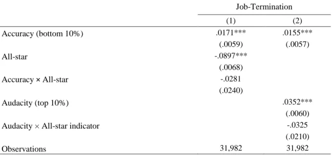
Table IV
Forecast Performance, All-Stars and the Likelihood of Job-Termination
This table presents records for the impact of analysts’ past forecast performance on their future probability of experiencing job-termination, depending on whether analysts are all-stars from 1997 to 2013. Being an all-star implies that an analyst is part of the All-America Research Team in a given year. We consider analysts’ past earnings forecasts to compute the forecast accuracy and audacity scores. In columns (1) and (2) the dependent variable is job-termination - analysts stop producing forecasts to I/B/E/S in the year to follow. The regressions are Equations (5) and (6). The standard errors are in parentheses. The symbols ***, **, * represent the 1%, 5% and 10% significance levels, respectively.
Job-Termination (1) (2) Accuracy (bottom 10%) .0171*** .0155*** (.0059) (.0057) All-star -.0897*** (.0068) Accuracy × All-star -.0281 (.0240) Audacity (top 10%) .0352*** (.0060)
Audacity × All-star indicator -.0325
(.0210)
Observations 31,982 31,982
In column (1) of Table IV we observe that for analysts that are non-all-stars, being in the 10th percentile of the forecast accuracy score increases the likelihood of leaving the sample by around 2%. Moreover, the coefficient on the all-star term is negative and statistical significant, denoting that all-stars are 9% less likely to leave the job than any other analyst. Finally, the interaction estimate indicates that weak accuracy is less relevant for all-stars. If an analyst has the all-star status, being in the 10th percentile of
27 the accuracy score reduces an analyst’s likelihood of being terminated by around 3% compared to other analysts also with low scores on accuracy.
We estimate Equation (6) plus the analyst feature 𝑎𝑙𝑙 − 𝑠𝑡𝑎𝑟𝑖,𝑡 and an interaction term. Column (2) of Table IV presents the estimates, indicating how job-termination varies with audacity for all-star analysts. Non-all-star analysts in the 10th percentile of the forecast audacity ranking have a 3.5% higher probability of job-termination. The coefficient on the interaction term is negative, indicating that an all-star analyst on the top 10% of the audacity score is less likely to be terminated than her counterparts, but is not statistically significant.
F. Employment outcome and forecast behaviors by sample periods
Additionally it is also interesting to observe how the association between employment outcomes and past forecast performance has varied over time. Previous literature argues that analysts face different incentives regarding accuracy and audacity when producing earnings forecasts since the beginning of the 21st century, after the implementation by the SEC of a set of ‘fair disclosure’ regulations that aim to stop the practice of selective publication (Agrawal et al. (2006)), leading analysts to change their practices.
To observe the reward for an analysts’ strong performance in the period between 2003 and 2013 and earlier periods, we use the same regression as in Section IV B. (Equation (5) plus 𝑒𝑥𝑝𝑒𝑟𝑖𝑒𝑛𝑐𝑒𝑖). We add a variable entitled 𝑎𝑓𝑡𝑒𝑟 2003𝑖 and an interactive variable with the forecast measures. 𝐴𝑓𝑡𝑒𝑟 2003𝑖 is equivalent to one if the estimation is from the year of 2003 and onwards, zero otherwise.
Column (1) of Table V presents the estimates considering as the dependent variable an analyst experiencing job-termination. An analyst that performs weakly in forecasting i.e. is in the 10th percentile of the accuracy rank, in the period before 2003 is 3% more
28 likely to experience job-termination than her counterparts. The estimate on the interaction term is negative and statistically significant, meaning that weak performance is less relevant for the likelihood of job-termination for the group of analysts producing forecast between 2004 and 2013. An analyst in the 10th percentile of the accuracy ranking from 2003 onwards, has a likelihood of job-termination 4% lower, comparing to the earliest period. Both coefficients are statistically significant. We conclude that accuracy is less relevant for employment outcomes in 2004 to 2013 than in previous periods.
Table V
Forecast Performance, Sub-Periods and the Likelihood of Employment Outcome
This table presents records for the impact of analysts’ past forecast performance on their future employment outcome for the periods of 1987 to 2003 and 2003 to 2013. We consider analysts’ past earnings forecasts to compute the forecast accuracy and audacity scores. In columns (1) and (2) the dependent variable is job-termination - analysts stop producing forecasts to I/B/E/S in the year to follow. In columns (3) and (4) the dependent variable is job-upgrade – analysts move to a high-status brokerage in the year to follow. The regressions are Equations (5) and (6). The standard errors are in parentheses. The symbols ***, **, * represent the 1%, 5% and 10% significance levels, respectively.
Job-Termination Job-Upgrade (1) (2) (3) (4) Accuracy (bottom 10%) .0295*** .0004 (.0095) (.0041) Accuracy × After 2003 -.0392*** -.0044 (.0121) (.0051) Audacity (top 10%) .0471*** -.0020 (.0069) (.0030) Audacity × After 2003 -.0514*** .0133*** (.0126) (.0053) Observations 31,982 31,982 28,590 28,590
We also observe the evolution of the sensitivity of employment outcomes to audacity over time. We estimate Equation (6) and add again the indicator 𝑎𝑓𝑡𝑒𝑟 2003𝑖. In column (2) of Table V the dependent variable is again whether an analyst leaves the job. Analysts producing earnings forecasts in the period before 2003 that are in the 90th percentile of the forecast audacity score are about 5% more likely to experience
job-29 termination. Thus, the interaction term is negative and statistically significant, indicating that audacity is more important to avoid an analyst’s likelihood of experiencing job-termination in the most recent years, from 2004 to 2013. For an analyst producing forecasts in the period of 2004 to 2013, being in the top of the audacity ranking reduces her likelihood of leaving the sample by about 5 percentage points.
In columns (3) and (4) of Table V we perform the same regression specifications as in columns (1) and (2) respectively now considering an analyst’s job-upgrade the dependent variable. Overall, an analyst in the top decile of the accuracy score is less likely to be upgraded in a more recent period than before the year of 2003. The estimate is neither economically nor statistically significant. In respect to the forecast audacity behavior, an analyst in the 90th percentile of the audacity score is 1% more likely to experience job-upgrade in the 2004 to 2013 period than before.
We conclude that from 2004 onwards forecast accuracy has less importance on the probability of job-termination and job-upgrade, while being bolder slightly indicates an increased likelihood of job-upgrade for the same period. Our results indicate a slight change in the relationship between forecast behaviors and employment outcomes after the year of 2003. Thus, the observed change in analysts’ outcome-performance relationship may not only be influenced by the impact of new regulation in the early 2000’s, but also by other reasons that we do not include in our research.
V. Conclusions
In our study we analyze the relation between employment outcome and the earnings forecasts of U.S. sell-side analysts submitted to I/B/E/S. We draw the following conclusions from our research.
30 When examining the impact of analysts’ past performance on employment outcome we conclude that, contrary to financial press and regulators judgments, an analyst’s career outcome is influenced by her ability to produce accurate earnings forecasts. In addition, controlling for forecast accuracy, an analyst’s tendency to diverge from the average forecasts (i.e. produce bold forecasts) is also considered by investment firms when defining analysts’ future outcome. Especially, analysts producing bold forecasts are more likely to experience job-termination. Moreover, we also find that inexperienced and experienced analysts have distinct incentives. Analysts performing weakly, i.e. with less accurate or bolder forecasts, but with experience are less likely to experience job-termination than inexperienced analysts. Thus, while past performance is a strong indicator of analysts’ forecasting ability for the youngest, with experience analysts’ ability may be assessed differently.
Furthermore, we identify in our sample of I/B/E/S analysts a group of all-stars. We analyze the impact of forecast performance, both accuracy and audacity, on the likelihood of job-termination and observe that this impact is absent for all-stars. We conclude that all-stars are less likely to experience job-termination than our regular sample of analysts. Thus, our results can be justified by the fact that, most likely, accuracy is already implicit and expected in a forecast of an all-star, hence other characteristics may impact the career outcome of the latter. The possibility of acquiring a larger sample of all-stars and deepen our analysis on the latter is a conjecture to consider on a further research.
Finally we find evidence that with the implementation of new regulation in the early 2000’s, job-termination becomes less sensitive to precision and job-upgrade slightly more sensitive to audacity. The regulations introduced in the years between 2000 and 2003 were mostly aimed at putting an end on several conflicts of interest
31 between firms, investment banks and other participants in the Wall Street, culminating with the Global Settlement of 2003. The diminishing impact of forecast accuracy on employment outcome, namely job-termination, after the implementation of the regulation measures is an interesting topic both from an academic and policy perspective. While in our analysis we divide the sample in two periods and point out the asymmetries in the outcome-performance relationship before and after the year of 2003; there is room for a lot more to be done regarding the different regulations implemented since then. We leave this issue for future research.
32
References
Alford, Andrew W., and Philip G. Berger, 1999, A Simultaneous Equations Analysis of Forecast Accuracy, Analyst Following, and Trading Volume, Journal of Accounting,
Auditing & Finance 14, 219-240.
Agrawal, Anup, Sahiba Chadha, and Mark A. Chen, 2006, Who is afraid of reg FD? The behavior and performance of sell‐side analysts following the SEC’s fair disclosure rules,
Journal of Business 79, 2811-2834.
Bernhardt, Dan, Murillo Campello, and Edward Kutsoati, 2006, Who herds?, Journal of
Financial Economics 80, 657–675.
Boni, Leslie, and Kent L. Womack, 2006, Analysts, Industries and Price Momentum, Journal of
Financial and Quantitative Analysis 41, 85-109.
Boris, Groysberg, Paul M. Healy, and David A. Maber, 2011, What drives sell-side analyst compensation at high-status investment banks?, Journal of Accounting Research 49, 969-1000.
Bhojraj, Sanjeev, Charles M. C. Lee, and Derek K. Oler, 2003, What’s my line? A comparison of industry classification schemes for capital market research, Journal of Accounting
Research 41, 745-774.
Brown, Lawrence D., Andrew C. Call, Michael B. Clement, and Nathan Y. Sharp, 2013, Inside the “black box” of sell-side financial analysts, Working paper.
Clarke, Jonathan, Ajay Khorana, Ajay Patel, and Raghavendra P. Rau, 2007, The impact of all-star analyst job changes on their coverage choices and investment banking deal flow’,
Journal of Financial Economics 84, 713-737.
Clement, Michael B., 1999, Analyst forecast accuracy: Do ability, resources, and portfolio complexity matter?, Journal of Accounting and Economics 27, 285-303.
Clement, Michael B., and Senyo Y. Tse, 2003, Do Investors respond to analysts' forecast revisions as if forecast accuracy is all that matters?, Accounting Review 78, 227-249. Clement, Michael B., and Senyo Y. Tse, 2005 Financial analyst characteristics and herding
behavior in forecasting, Journal of Finance 60,307–341.
Cliff, Michael T., and Denis, David J., 2004, Do initial public offering firms purchase analyst coverage with underpricing?, Journal of Finance 59, 2871–2901.
Cohen, Lauren, Andrea Frazzini, and Christopher Malloy, 2010, Sell-side school ties, Journal of
Finance 65, 1409–1437.
Francis, Jennifer, Qi Chen, Richard H. Willis, and Donna R. Philbrick, 2004, Security Analyst Independence, The research foundation of CFA institute.
Gu, Zhaoyang, and Joanna Shuang Wu, 2003, Earnings skewness and analyst forecast bias,
Journal of Accounting and Economics 35, 5-29.
Holmstrom, Bengt, 1999, Managerial incentive problems: A dynamic perspective, Review of
Economic Studies 12, 95–129.
Hong, Harrison, Jeffrey D. Kubik, and Amit Solomon, 2000, Security analysts' career concerns and herding of earnings forecasts, RAND Journal of Economics 31, 121-144.
Hong, Harrison, and Jeffrey D. Kubik, 2003, Analyzing the analysts: Career concerns and biased earnings forecasts, Journal of Finance 2003, 313-351.
Irvine, Paul J., 2004, Analysts' Forecasts and Brokerage‐Firm Trading, Accounting Review 79, 125-149.