A Work Project, presented as part of the requirements for the Award of a Master´s Degree in Finance from the NOVA – School of Business and
Economics
Interconnectedness of the Insurance Sector
with the
Banking and Non-financial Sectors
Ana Silva 2328
A Project carried out on the Master in Finance Program, under the supervision of:
Professor Paulo Manuel Marques Rodrigues
Abstract
This work project studies the interconnectedness of the European insurance sector with
the banking and non-financial sectors through both a VAR model (together with the Granger causality test) and a Markov Switching model. I concluded that after the crisis,
the existing linkages between institutions were more numerous than the ones that were detected prior to it. Evidence suggests that banks´ past returns began to Granger cause the returns of insurance companies and vice-versa only after the crisis. Lastly, it was seen
that the interconnectedness among individual insurance companies during the 2008 crisis became stronger.
Keywords: systemic risk, interconnectedness, insurance, Granger causality
1.
Introduction
If banks are considered to play a central role in the financial system, then so are
insurance firms since they enable households and other companies to transfer risks to a third party. Until recently, banks were considered the most important source of systemic
risk. The banking sector inherently presents a greater level of systemic risk, which is mainly due to its extensive degree of interconnectedness. This ultimately translates into a domino effect that may be easily triggered by the failure of a single bank. Such an
apparently isolated event may send out irreversibly damaging ripples to the entire industry. Additionally, banks are highly susceptible to liquidity issues and bank runs. This is because their balance sheets are normally characterized by what is known as an
asset-liability mismatch (assets are long-term while liabilities are short-term). This means that
they fund their mortgages with short-term deposits, assuming they may be rolled over.
Insurance companies are theoretically far less prone to systemic risk since they are
not as vulnerable to customer runs, which could only occur if all clients had the appropriate claims to do so. In any case, insurance companies are not responsible for the creation of liquidity, a payment system or capital lending. Liquidity complications are
easier to avoid since the maturity of the insurer´s assets is less than the maturity of their liabilities (no asset-liability mismatch exists). Nevertheless, the insurance sector is
beginning to play an increasingly more important role in contributing to the levels of systemic risk in general, as will be demonstrated later on.
Despite all this, when we think of insurance companies we tend to see them as a source of stability for the financial system (as the up-front premiums allow insurers to have a strong operating cash-flow). However, after the financial crisis of 2008-2009, and
particularly after AIG’s crisis1, the possible contribution of the insurance sector to the levels of systemic risk has become a more relevant topic of discussion.
According to FSB (financial stability board) systemic risk refers to the potential hindrance in the delivery of financial services that may be caused by either the failure of parts or of the entire financial system itself, having the power to inflict serious
consequences to the whole economy. That is, systemic risk can be described as the collapse of an entire system, where the malfunctioning of an individual institution can
cause a cascading failure of the whole system. This overall breakdown happens due to the high level of interconnectedness (link or the interdependence) among financial institutions.
1According to McDonald
et al (2014), AIG lost 99.2$ billions of its assets merely in 2008. This company received a
I have decided to focus my work on one of the indicators of systemic risk of the
insurance sector, namely on the inter and intra-insurance sector interconnectedness. I have chosen this topic because systemic risk is extremely important and can affect the financial system as well as the real economy at various levels. First, bank runs lead to the
scarcity of capital supply and may cause the bankruptcy of illiquid institutions (despite the possibility of them being solvent) or even of households. Second, the disruptions in
credit flows may cause a decline in the amount of capital available to finance investments. Finally, systemic risk can ultimately lead to the decline in wealth and to the increase in uncertainty, which can cause a reduction of economic activity.
IAIS established in 2013, five indicators that can measure the relative systemic importance of a specific insurer. These are: non-traditional/non-insurance activities,
interconnectedness, size, global activity and substitutability.
The size (measured by the insurer´s total assets and/or total revenues), substitutability (existence/effectiveness of an insurer´s substitute products) and global activity indicators
(the insurer´s exposure to other countries) are the least systemically relevant of all. As a result, each one contributes with only a 5% weight.
The extent and complexity of non-traditional activities represent a weight of 45% and as we saw before it can lead to serious financial losses (as in the AIG case). Having said
that, I will mainly focus on the degree of interconnectedness between insurers, banks and non-financial firms (which contributes, according to the IAIS, with a weight of 40% in the measurement of an insurer´s systemic importance).
The Financial Stability Board (FSB) has been working incessantly to develop studies related to the systemic risk of banks and insurers. In 2013 it published, along with the
collaboration of IAIS, a global list of systemically relevant insurers (G-SII). In other
and its members are expected to implement several measures whose objective is to reduce
the probability and impact of a potential failure of the G-SIIs by making them less systemically relevant. In 2016 this list includes insurers such as Allianz SE, Axa S.A., MetLife Inc., Prudential plc and American International Group Inc.
My goal in this paper is to evaluate the interconnectedness between the banking, insurance and non-financial industries. One of the measures of interconnectedness that I
focus on is the linear Granger causality test proposed by Bilio et al. (2012). Correlation
does not imply causality and therefore I chose to apply this method because I believe that determining the direction of the linkages between firms is as important as investigating
the degree of interconnectedness between those same institutions. This information is critical when deciding which measures to apply and to which companies they should be
applied to in order to reduce the systemic risk associated with those connections. If a regulator is able to distinguish between companies that are responsible for the systemic
risks and those that are “victimized” by them, then more effective measures may be
implemented. I will also analyze how the degree of interconnectedness evolved before and after the 2008 financial crisis. Furthermore, this work contributes to the study of the
intra-sector interconnectedness through the same VAR model’s structure and Granger causality tests.
It is known that oil prices influence the real economy (see e.g. Hamilton (1983) or Jimenez-Rodriguez and Sanchez (2005)) but also the stock market (e.g. Nandha and Faff (2008) and Shimon and Raphael (2006)). Therefore, I have decided to include as an
explanatory variable of the institutions’ stock returns the oil price returns in order to correct for global effects on stock returns, which is a novel approach considered here. On
10-year swap rate, as explanatory variables. More than a methodological contribution, my
contribution resides in the new evidence I found about this topic.
This thesis will begin by reviewing the existing literature related to systemic risk and their respective measures. It will also detail the existing methods of analysis used to study
the degree of interconnectedness between financial institutions (section 2). Afterwards, I shall provide information regarding the data and methodology used (section 3 and 4) as
well as an analysis of my results (section 5). Finally, I will present concluding remarks (section 6).
2.
Literature review and Methodology
The present section aims to provide a theoretical overview of the topic of systemic
risk and respective measures and to present the methodologies applied throughout this research.
2.1Systemic Risk and Insurance Companies
A minority of authors, namely Bierth et al. (2015) defend that systemic risk in the insurance industry is quite small (although the insurance sector’s contribution to systemic
risk has peaked during the financial crisis). According to them, whenever existent, this
contribution to systemic risk is due to the “leverage, loss ratios and funding fragility” of
insurers. They reached this conclusion using a sample of 253 life and non-life insurers
between 2000 and 2012.
On the one hand, the majority of the existing literature about systemic risk in the
insurance industry agrees that insurers engaging in traditional activities, even the large ones, present a low systemic risk. On the other hand, the potential impact on systemic
to present more details of current literature on this topic, it is crucial to understand the
differences between traditional and non-traditional insurance activities.
According to IAIS 2011, traditional activities are the core of the insurance business. Underwriting life and health risks (within the life insurance sector) and legal, liability,
accident and property risks (within the non-life insurance sector) are considered traditional activities. Underwriting reinsurance is also considered as a conventional
activity.
Non-traditional activities are for instance financial guarantee insurance,
insurance-linked securities (ILS), cascades of repos and securities lending. According to IAIS, CDS/CDO underwriting, capital market business, banking (including investment banking and hedge funds activities), third-party asset management and industrial activities are
considered insurance activities. However when most of the authors refer to non-traditional activities they are including those noninsurance in the same package.
In Geneva Association’s opinion, from its 2010 report, it is more important for
regulators to assess the systemic risk of the insurer’s activities than to identify the
institutions that present systemic risk. They defend that since they conclude through their
study that the traditional activities of the insurers and reinsurers do not pose systemic risk, that it is the non-core and quasi-banking activities like “derivatives trading on non
-insurance balance sheets and mis-management of short term funding from commercial
paper or securities lending” that present systemic risk. Therefore, the contribution of a
specific company to the systemic risk does not depend on the company itself but on the
type of activities that the company does. Other authors, like Cummins and Weiss (2011) and Trichet (2005), share this point of view. This is also the point of view adopted by the
2.2Interconnectedness between insurers, banks and non-financial institutions
Interconnectedness may be understood as the existing systemic linkage between two
parties. This concept has become extremely important and has been the target of multiple studies.
In general terms, there are four models that measure the linkages between financial institutions: Principal components, MES (Marginal Expected Shortfall), DIP (Distressed Insurance Premium), and Granger causality tests.
Neale et al. (2012) used principal component analysis to measure the existing linkages between insurance companies. They also apply Granger causality tests to their sample of
US financial institutions in order to analyze the interconnectedness between these firms. They concluded that the connections among financial institutions have been actively increasing. Additionally, these linkages differ according to the type of industry
(insurance, banks, brokers, hedge funds and financial holding companies). Within the insurance industry, interconnectedness among financial institutions is strongest for
insurers that commercialize warranties and life insurance. In that sense, those companies are more prone to pose systemic risk. The Granger causality test developed by Billio et
al. (2012) can measure not only the degree of interconnectedness but also the direction of
shocks.
Chen et al. (2013) applied the Granger causality test to US banks and insurers and
concluded that the former produce an important systemic risk for insurers. On other hand, the impact of insurers on banks is not significant in the US market, which makes insurers shocks sufferers. Due to the high level of systemic risk inherent to the banking industry,
they additionally defend that regulators ought to allocate their efforts towards minimizing the impact of banks´ systemic risks on insurers (namely through investment and capital
When using Granger causality tests to test for interconnectedness, it relies on the
market returns of banks, insurers and non-financial companies and its respective market capitalizations. The benefit of using equity-based measures is that equity markets constantly react to new public information available about those companies which is
reflected in its respective stock prices quicker than it would be reflected in other nonmarket-based variables.
Berdin and Sottocomola (2015) arrived at the same conclusion after applying Granger causality tests to European institutions. They postulate that non-financial institutions were the main originators of systemic risk prior to the financial crisis. Post-crisis, banks became
the main contributors of this type of risk (and by opposition financial institutions were net receivers before crisis and non-financial institutions net receivers after the crisis).
Apart from that, the systemic risk is greater for companies that exercise non-traditional insurance activities. The authors state that insurers mostly played a subordinated role when compared to banks, especially during the financial crisis. Acharya et al. (2011)
proposed the SES (systemic expected shortfall) to measure the return of an institution when the system is in a recession and also concluded that the non-traditional activities of
the insurers generate systemic risk. These authors defend that non-traditional insurance products should be fully capitalized and if that is not possible, they should be forbidden.
They also defend that companies that present systemic risk should pay a fee that will be used to rescue those companies in case of a systemic crisis.
2.3
The Granger Causality TestThe Granger causality test was originally proposed by Granger (1969) and later on
disseminated by Sims (1972). According to this test, a random variable 𝑋 Granger causes
another random variable 𝑌 if the past values of 𝑋 can contribute to predict 𝑌 with a better
coefficient 𝑑 in (2) is statistically significant so as to predict X. In other words, consider
the model
𝑌𝑡= 𝑎 𝑌𝑡−1+ 𝑏 𝑋𝑡−1+ 𝑢𝑡 (1)
𝑋𝑡= 𝑐 𝑋𝑡−1+ 𝑑 𝑌𝑡−1+ 𝑣𝑡 (2)
where X and Y are two stationary variables with zero mean, 𝑢𝑡 and 𝑣𝑡 are two
uncorrelated white noise processes. 𝑎, 𝑏, 𝑐 and 𝑑 are the model coefficients.
In the case that X Granger causes Y as well as Y Granger causes X, we have a feedback relationship between these two variables.
The choice of the optimal number of lags is of extreme importance since we can compromise the accuracy of the test (if we choose too many) or allow for autocorrelated errors (if we choose to few) and therefore obtain misleading test results. In the present
work, the method described above will be used in order to measure the interconnectedness between the companies.
2.4Markov-Switching Model
We can observe that for financial data from time to time there is a switch in the pattern of the data both at an expected return level and at a volatility level.A linear model such as a VAR model is incapable of capturing the regime-switching nature that may
characterize financial data. Therefore, Hamilton (1989) proposed the Markov switching model or regime-switching model, which is a non-linear time series model. According to
this model, all possible occurrences distribute themselves into 𝑚 states/regimes of the
world called 𝑠𝑡, 𝑡 = 1, … , 𝑚. The Markov switching model is composed of as many
equations as the number of regimes that are being analyzed, so each equation corresponds to a different regime/pattern.
A switching model for the variable 𝑟𝑡 that follows a first-order Markov chain, in which
𝑟𝑡=∝0+∝1 𝑠𝑡+ 𝛽𝑟𝑡−1+ 𝜀𝑡 (3)
where 𝑟𝑡 is the return of a specific group for period t (e.g. insurance companies or banks),
𝑟𝑡−1is the return of this group for the period t-1; ∝0 is the state-independent intercept, ∝1
is the state-dependent intercept and 𝑠𝑡 is an unobservable dummy state variable that
assumes the value of 1 in the state where the volatility is larger and assumes the value of
0 in the lower volatility state. Similarly, the probability of the current state, 𝑗, only
depends on the previous state:
𝑃(𝑆𝑡 = j|𝑆𝑡−1 = i, 𝑆𝑡−2 = k, 𝑆𝑡−3= w. . . ) = P(𝑆𝑡 = j|𝑆𝑡−1 = i) = 𝑝𝑖𝑗 (4)
𝑝𝑖𝑗 can be defined as the “probability of being in state 𝑗 in the current period given that
the process was in state 𝑖 in the previous period”.
We will obtain different parameters for each state, as well as the transition probability from one state to the other. An advantage of this model is that the variable 𝑠𝑡 is not defined
by the user in the sense that it is not observable, but is inferred through the behaviour of
the dependent variable, in this case 𝑟𝑡. The Markov-Switching model will be applied in this
work as an alternative to the VAR model in studying the interconnectedness between the companies.
3.
Data
Due to data availability issues, I chose to analyze the period between June 2000 and September 2016. I have created my own index of monthly returns from the biggest
European banks, insurers and non-financial companies with biggest average monthly market cap that were listed since June 2000 and belong to the EuroStoxx 600 Insurers, Banks or Price (that combine the biggest financial and non-financial institutions listed in
Europe at the time data was collected) Indices. This index is calculated by summing the
companies that I have considered for the analysis as well as a summary of related
descriptive statistics are presented in Tables 1, 2 and 3 of Appendix 1.
In order to test for the interconnectedness between institutions, I decided to use company returns at a monthly frequency in order to avoid complex heteroscedasticity
problems associated with market returns at higher frequencies. With respect to insurance companies and banks, I have included all institutions for which I had available data, 25
and 34 companies, respectively. Regarding the non-financial companies, I included the 40 biggest. In relation to the split non-financial industries, I have considered the 15
biggest of each group since in measuring the interconnectedness among the institutions I want to focus mainly on the biggest companies. The indices for those split non-financial companies were calculated in the same way as described before for the banks and insurers
indices. All data was downloaded from Bloomberg. I have also downloaded the Brent crude oil prices, the 1-month Euribor and the 10-years swap rate from the Bloomberg
terminal.
4.
Empirical Results
This section will begin by summarizing some of the most relevant descriptive
statistics related to financial and non-financial companies’ returns. Besides this, it will also analyse the results of the econometric models applied. I will consider a 5% significance level.
4.1 Stationarity of variables – Dickey-Fuller Test
According to Brooks (2014), we should guarantee that the time series we are using
are stationarity before estimating a VAR model in order to see if the relation between the variables is meaningful.
As the stock returns are by nature stationary variables (which can also be confirmed
2), I perform a Dickey-Fuller test on those variables just for confirmation (Appendix 3).
Next, I will also test the nonstationarity of Brent price, 1M-Euribor and 10 years Swap rate with a Dickey-Fuller test (Appendices 3.4 to 3.6). I chose not to include a constant term within the DF test based on my perusal of the time series graphs (Appendix 2) and I
will apply a maximum of 14 lags and use the Schwartz criteria (BIC2) to select the model order. After performing the Dickey-Fuller test, results showed that all of the time series
were stationary except for the Brent price, the Euribor1M and the 10y swap rate (Appendix 3). It is worth mentioning, however, that the stationarity of these three variables may be guaranteed by taking their first differences. As such, I will consider the
first differences of the Brent price, the Euribor1M and the 10y swap rate from this point onward.
4.1 VAR Model for Banks, Insurers and Non-financial Companies
I have computed an unrestricted VAR (vector autoregressive) model with the
monthly returns of insurers, banks and non-financial institutions as my endogenous variables. With regards to exogenous variables, I have selected a dummy that is related to the crisis (with starting point in January 2008), the Brent crude oil price, the 1M Euribor
as a proxy to the short-term interest rate and finally the 10-year swap rate as a proxy for the long-term interest rate.
Equations 5, 6 and 7 represent the models to be estimated.
𝐵𝑎𝑛𝑘𝑠𝑡= 𝑐 + ∑ 𝛼𝑖𝐿𝑖𝐵𝑎𝑛𝑘𝑠𝑡 3
𝑖=1
+ ∑ 𝛽𝑖𝐿𝑖𝐼𝑛𝑠𝑢𝑟𝑒𝑟𝑠𝑡 3
𝑖=1
+ ∑ 𝛾𝑖𝐿𝑖𝑁𝑜𝑛𝑓𝑖𝑛𝑠𝑡 3
𝑖=1
+ 𝜃1𝐶𝑟𝑖𝑠𝑖𝑠𝑡+ 𝜃2∆ 𝐵𝑟𝑒𝑛𝑡𝑡+ 𝜃3∆ 𝐸𝑢𝑟𝑖𝑏𝑜𝑟𝑡+ 𝜃4∆ 𝑆𝑤𝑎𝑝𝑡+ 𝑢𝑡 (5)
𝐼𝑛𝑠𝑢𝑟𝑒𝑟𝑠𝑡= 𝑐′+ ∑ 𝛼𝑖′𝐿𝑖𝐵𝑎𝑛𝑘𝑠𝑡 3
𝑖=1
+ ∑ 𝛽𝑖′𝐿𝑖𝐼𝑛𝑠𝑢𝑟𝑒𝑟𝑠𝑡 3
𝑖=1
+ ∑ 𝛾𝑖′𝐿𝑖𝑁𝑜𝑛𝑓𝑖𝑛𝑠𝑡 3
𝑖=1
+ 𝜃1′𝐶𝑟𝑖𝑠𝑖𝑠𝑡+ 𝜃2′ ∆ 𝐵𝑟𝑒𝑛𝑡𝑡+ 𝜃3′ ∆ 𝐸𝑢𝑟𝑖𝑏𝑜𝑟𝑡+ 𝜃4′ ∆ 𝑆𝑤𝑎𝑝𝑡+ 𝑢𝑡′
𝑁𝑜𝑛𝑓𝑖𝑛𝑠𝑡= 𝑐′′+ ∑ 𝛼𝑖′′𝐿𝑖𝐵𝑎𝑛𝑘𝑠𝑡 3
𝑖=1
+ ∑ 𝛽𝑖′′𝐿𝑖𝐼𝑛𝑠𝑢𝑟𝑒𝑟𝑠𝑡 3
𝑖=1
+ ∑ 𝛾𝑖′′𝐿𝑖𝑁𝑜𝑛𝑓𝑖𝑛𝑠𝑡 3
𝑖=1
+ 𝜃1′′𝐶𝑟𝑖𝑠𝑖𝑠𝑡+ 𝜃2′′ ∆ 𝐵𝑟𝑒𝑛𝑡𝑡+ 𝜃3′′∆ 𝐸𝑢𝑟𝑖𝑏𝑜𝑟𝑡+ 𝜃4′′∆ 𝑆𝑤𝑎𝑝𝑡+ 𝑢𝑡′′ (7)
(6)
2 According to Brooks (2008), the BIC criteria is more consistent than the AIC criteria in the sense that it normally
I will estimate the models above for three distinct time horizons: the full sample
(June 2000 – September 2016), the pre-crisis (June 2000 – December 2007) and the post-crisis (January 2008 – September 2016) periods.
Upon estimating the VAR model above for the full sample and adjusting for the best
lag specification (Appendices 4.1 and 4.2), I have concluded that both autocorrelation and heteroscedasticity are present (Appendices 4.3 and 4.4 respectively).
Consequently, I will therefore estimate these models using a GMM-HAC approach in order to correct for both autocorrelation and heteroscedasticity using the appropriate
number of lags as indicated in Appendix 4.2.
By analyzing the results obtained from the GMM-HAC estimation at a 5% significance level (Appendix 4.5), the dummy linked to the crisis period seems to be
statistically insignificant and therefore irrelevant in explaining any of the returns from the three sets of companies, including the first difference of the 1M Euribor. As such, I have decided to remove both of these variables from my model and reestimated the VAR/HAC
model (Appendices 4.6 and 4.8).
The process described above was repeated for the samples before and after the crisis.
The following table presents the variables that resulted to be significant (** are used to signalize the variables that are statistically significant at a 5% significance level and with
Table 1: Coefficients of the VAR model estimated through the GMM-HAC method
The analysis of the model applied to the full sample time horizon reveals that, at a
5% significance level, the third lag of the insurers returns (in the period 𝑡 − 3) is
statistically significant to explain the banks and non-financial companies returns in period
𝑡. We can observe that there is a negative influence of the insurers past returns on the
banks and non-financial companies current returns (if that lag of insurers returns increase
in one percentage point, the banks and non-financial companies’ returns in moment 𝑡 decrease by 0.23 and 0.19 percentage points). Also, the second lag of the returns of the
non-financial companies (in period 𝑡 − 2) are indeed statistically significant and are
therefore able to explain the bank returns in period 𝑡 (direct relationship).
By dividing the study into two parts, the pre and post-crisis periods, one can conclude that within the pre-crisis period the lagged values of the returns of the insurance and
non-financial firms are not able to describe the bank returns. The opposite is not verified after the crisis, when the returns of these companies become statistically significant in
modeling the bank returns. Also, whereas before the financial crisis, there was no relationship between the banks and insurers returns, after the crisis, banks past returns
Full sample Before crisis After crisis Full sample Before crisis After crisis Full sample Before crisis After crisis 0.0026 0.0116 0.0039 0.0004 0.0029 0.0095 0.0054 0.0111 0.0090 0.2671 -0.2960 0.4398* 0.1418 -0.3552 0.4234** -0.0679 -0.5443** 0.1468
-0.1089 0.1310 0.0023 0.3042 -0.0804 0.0720
0.2706** 0.1876 0.1506 0.2067 0.1119 0.0970
-0.3596** -0.1794 -0.1648**
-0.2420 0.1193 -0.4072* -0.2114 0.0604 -0.4227** -0.0133 0.1854* -0.0757
-0.2617 -0.5131* -0.2427 -0.5006** -0.0304 -0.0436
-0.2345** -0.0783 -0.2256* -0.0895 -0.1909** 0.0109
0.6350** 0.5521** 0.4477**
0.1882 0.1672 0.1817 0.1997 0.2675 0.0919 0.1418 0.2372* 0.0268
0.3342** 0.3259* 0.1819 -0.0710 0.0563 -0.0840
0.2406 0.1693 0.3225 -0.1394 0.2707** -0.0755
-0.2361 -0.2673 -0.4159**
0** 0** 0** 0** 0** 0*
9.5299** 11.0580** 10.1037** 10.2910** 15.9491** 7.6818 6.8968** 11.4717** 4.1829*
Banks Insurers Non-financial companies
𝐵𝑎𝑛𝑘𝑠𝑡−1 𝐵𝑎𝑛𝑘𝑠𝑡−2 𝐵𝑎𝑛𝑘𝑠𝑡−3 𝐵𝑎𝑛𝑘𝑠𝑡−4 𝐼𝑛𝑠𝑢𝑟𝑒𝑟𝑠𝑡−1 𝐼𝑛𝑠𝑢𝑟𝑒𝑟𝑠𝑡−2 𝐼𝑛𝑠𝑢𝑟𝑒𝑟𝑠𝑡−3 𝐼𝑛𝑠𝑢𝑟𝑒𝑟𝑠𝑡−4 𝑁𝑜𝑛𝑓𝑖𝑛𝑠𝑡−1 𝑁𝑜𝑛𝑓𝑖𝑛𝑠𝑡−2 𝑁𝑜𝑛𝑓𝑖𝑛𝑠𝑡−3 𝑁𝑜𝑛𝑓𝑖𝑛𝑠𝑡−4 𝑐𝑟𝑖𝑠𝑖𝑠 ∆ 𝐵𝑟𝑒𝑛𝑡 𝑃𝑟𝑖𝑐𝑒𝑡
∆ 1 𝐸𝑢𝑟𝑖𝑏𝑜𝑟𝑡
∆ 1 wa a 𝑡
were able to explain (through a direct relationship) insurance companies’ current returns
and vice-versa.
Like bank returns, the returns of the insurance companies can only be explained by past returns of banks during the post-crisis period and not before. With respect to the
non-financial companies, one can conclude that their returns were only explained by the past bank returns before the crisis, but shortly thereafter the past returns of the banks and
insurance companies became statistically relevant in explaining the returns of the non-financial institutions.
The first difference of the 10y swap rate seems to be statistically significant in
illustrating the behavior of almost all companies’ current returns in both the pre and post-crisis periods. On the other hand, despite that the first difference of the Brent price is
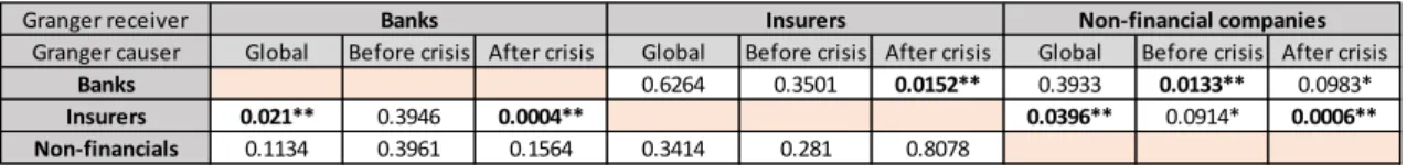
statistically relevant in describing all companies’ current returns, its coefficient assumes the value of zero and therefore the impact of this variable on the returns is very small. The Granger causality tests presented in the table below (Appendices 4.9, 5.9 and
6.9) based on a 5% significance level show that before the crisis the only existent interconnection was among banks and non-financial companies (banks past returns
Granger cause those last companies’ current returns). For the full and especially post-crisis samples, the relationships between companies became more numerous: past returns
of the insurance companies Granger cause both the current returns of the banks and non-financial companies. Besides that, banks possess a causal relation with the post-crisis returns of the insurance firms.
Table 2: P-values of Granger causality tests
Granger receiver
Granger causer Global Before crisis After crisis Global Before crisis After crisis Global Before crisis After crisis
Banks 0.6264 0.3501 0.0152** 0.3933 0.0133** 0.0983*
Insurers 0.021** 0.3946 0.0004** 0.0396** 0.0914* 0.0006**
Non-financials 0.1134 0.3961 0.1564 0.3414 0.281 0.8078
It can be concluded that before the crisis, banks were Granger causers of the
non-financials current returns whereas after the crisis banks started to Granger cause also the current insurers’ returns. The opposite also applies, that is, in the post crisis period, the insurers’ past returns Granger cause not only the non-financial companies’ returns but
also the banks’ returns (there was a feedback relationship between banks and insurers returns).
5.2 VAR Model for Financial and Non-financially Split Industries
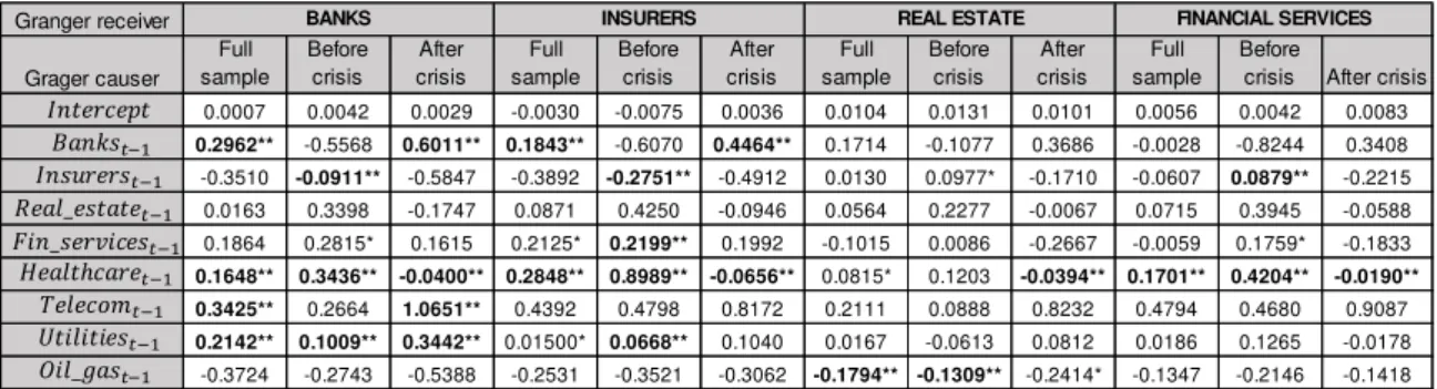
Table 3: Coefficients of the VAR model estimated through the GMM-HAC method
Table 4:Coefficients of the VAR model estimated through the GMM-HAC method
(table 3 continuation)
By observing the tables above that summarize the coefficients of the models presented in Appendices 7.1 to 7.3, one can conclude that before the crisis the current insurers returns were mainly the Granger receivers of the shocks namely form real estate,
healthcare, telecom and oil and gas companies’ past returns. However, after the financial crisis, the insurance companies’ past returns became the Granger causers of the current
returns of the banks, telecom and utilities companies.
Granger receiver Grager causer Full sample Before crisis After crisis Full sample Before crisis After crisis Full sample Before crisis After crisis Full sample Before
crisis After crisis
0.0007 0.0042 0.0029 -0.0030 -0.0075 0.0036 0.0104 0.0131 0.0101 0.0056 0.0042 0.0083 0.2962** -0.5568 0.6011** 0.1843** -0.6070 0.4464** 0.1714 -0.1077 0.3686 -0.0028 -0.8244 0.3408 -0.3510 -0.0911** -0.5847 -0.3892 -0.2751** -0.4912 0.0130 0.0977* -0.1710 -0.0607 0.0879** -0.2215 0.0163 0.3398 -0.1747 0.0871 0.4250 -0.0946 0.0564 0.2277 -0.0067 0.0715 0.3945 -0.0588 0.1864 0.2815* 0.1615 0.2125* 0.2199** 0.1992 -0.1015 0.0086 -0.2667 -0.0059 0.1759* -0.1833 0.1648** 0.3436** -0.0400** 0.2848** 0.8989** -0.0656** 0.0815* 0.1203 -0.0394** 0.1701** 0.4204** -0.0190** 0.3425** 0.2664 1.0651** 0.4392 0.4798 0.8172 0.2111 0.0888 0.8232 0.4794 0.4680 0.9087 0.2142** 0.1009** 0.3442** 0.01500* 0.0668** 0.1040 0.0167 -0.0613 0.0812 0.0186 0.1265 -0.0178 -0.3724 -0.2743 -0.5388 -0.2531 -0.3521 -0.3062 -0.1794** -0.1309** -0.2414* -0.1347 -0.2146 -0.1418
BANKS INSURERS REAL ESTATE FINANCIAL SERVICES
𝐵𝑎𝑛𝑘𝑠𝑡−1
𝑖𝑛 𝑠𝑒𝑟𝑣𝑖𝑐𝑒𝑠𝑡−1 𝑒𝑎 𝑡 𝑐𝑎𝑟𝑒𝑡−1
𝐼𝑛𝑠𝑢𝑟𝑒𝑟𝑠𝑡−1
𝑒 𝑒𝑐𝑜𝑚𝑡−1 𝑡𝑖 𝑖𝑡𝑖𝑒𝑠𝑡−1 𝑖 𝑎𝑠𝑡−1 𝑒𝑎 𝑒𝑠𝑡𝑎𝑡𝑒𝑡−1
𝐼𝑛𝑡𝑒𝑟𝑐𝑒𝑝𝑡 Granger receiver Grager causer Full sample Before crisis After crisis Full sample Before crisis After crisis Full sample Before crisis After crisis Full sample Before
crisis After crisis
0.0068 0.0002 0.0100 -0.0012 -0.0042 0.0037 0.0066 0.2036 -0.0042 0.0023 0.0037 -0.0007 0.0098 0.0458** -0.0202 -0.0963 -1.0921 0.2290** 0.0981 -0.3334 0.2425** 0.0640 -0.1846 0.1359 -0.0912* -0.2093** 0.0225 -0.1487 0.0687* -0.2766 -0.1352 0.1602 -0.3505 -0.0435 -0.0125 -0.0508 0.0989 0.1951 -0.0237 0.1020 0.2714 0.0353 0.0033 0.0015 0.0340 0.1054 0.0983 0.0802 0.0873 0.0875 0.1017 0.0553 0.3266 -0.0968 0.0579 -0.0371 0.1100 0.0598 0.0644** 0.0686 0.0012** 0.1625* -0.0763** 0.1179 0.2431** -0.0127** -0.0228** 0.1144** -0.0841** 0.1125** 0.3461** 0.0068**
0.1600 0.1070 0.4075 0.2114** 0.2402** 0.3993 0.2759 0.2248* 0.6898 0.2621 0.1996 0.6290 0.0206 0.0779 0.0303 0.1552** 0.4618** -0.0013 0.1209 0.2219 -0.0191 -0.0035** 0.1452** -0.1183** -0.1000** -0.1364 -0.1450** -0.2228 -0.6130 -0.0391 -0.0132 -0.1345** 0.0043 -0.2365 -0.2936 -0.2785
HEALTHCARE TELECOM UTILITIES OIL AND GAS
𝐵𝑎𝑛𝑘𝑠𝑡−1
𝑖𝑛 𝑠𝑒𝑟𝑣𝑖𝑐𝑒𝑠𝑡−1
𝑒𝑎 𝑡 𝑐𝑎𝑟𝑒𝑡−1
𝐼𝑛𝑠𝑢𝑟𝑒𝑟𝑠𝑡−1
𝑒 𝑒𝑐𝑜𝑚𝑡−1
𝑡𝑖 𝑖𝑡𝑖𝑒𝑠𝑡−1
𝑖 𝑎𝑠𝑡−1
𝑒𝑎 𝑒𝑠𝑡𝑎𝑡𝑒𝑡−1
Within the financial sector, the insurance, health care, telecom, utilities and oil and gas
industries past returns Granger cause the banks’ returns. Only before the crisis, did real estate past returns Granger cause the banks, insurers, financial services and healthcare current returns. Those interconnections disappeared after the financial crisis, when banks
and telecom companies’ past returns started to Granger cause the real estate companies’ current returns. With respect to the financial services companies, before the crisis, they
act as Granger receivers of the shocks from the banks, real estate and telecom companies and the interconnection with the telecom companies was the only one that persisted in the post crisis period.
When analyzing the full sample, banks and insurers as well as the financial services industries were mainly the receivers of the shocks from the remaining industries.
Curiously, telecom companies seem also to have had an important role as their past
returns Granger cause all other companies’ current returns, both before and after the crisis.
After the crisis, banks and insurers started to act as Granger causers. For example,
the past returns of both banks and insurers Granger cause basic materials and telecom industries’ returns; bank past returns granger cause real state, insurers and financial
services industries returns insurers past returns Granger cause the utilities industry returns.
By observing this data one can conclude that besides the interconnectedness that exists among the financial institutions, namely banks and insurers, it can also be found between financial and non-financial industries.
5.3 Markov Switching Model
Some abrupt changes from time to time can be observed in financial time series in a
equity returns that occurred in 2008 due to the financial crisis, but like this example there
may be several others. Consequently, it is more logical to estimate my model through a Markov switching model with two regimes, in which the regime with greatest volatility is associated with the crisis periods. The advantage of using this method instead of a
dummy variable is that by using the latter we are limited to dividing our sample into two sub-periods (in this case periods with and without crises). Per contra, by using this model,
if in any given period within our sample there exists a time span with a similar pattern as
the one from the 2008 crisis, then they will be grouped into the same “regime”. This
enables us to capture more complex dynamic patterns. The disadvantage of using this
method is that as I am working with monthly observations (196 on total), I will end up with a relatively small number of observations in each regime and therefore the resulting
estimates may not be as accurate as intended due to the small number of observations. When applying this model to my sample (see Appendix 8), it can be observed in the graph below that the following observations belong to the regime of largest volatility,
regime 2: April to August 2001; January 2002 to May 2003; May 2008 to June 2009 (the well-known 2008 financial crisis) and April 2011 to August 2011.
Graph 1: Markov-Switching model graph
Below are the results of this estimation.
Regime 1 (lower volatility)
{
𝐵𝑎𝑛𝑘𝑠𝑡= , 3− ,1 𝐵𝑎𝑛𝑘𝑠𝑡−1− ,32 𝐵𝑎𝑛𝑘𝑠𝑡−2− , 6 𝐼𝑛𝑠𝑢𝑟𝑒𝑟𝑠𝑡−1− , 2 𝑁𝑜𝑛𝑓𝑖𝑛𝑠𝑡−1+ ,28 𝑁𝑜𝑛𝑓𝑖𝑛𝑠𝑡−2+ 𝑢1,𝑡
𝐼𝑛𝑠𝑢𝑟𝑒𝑟𝑠𝑡= , 3 + , 5 𝐵𝑎𝑛𝑘𝑠𝑡−1+ ,18 𝐵𝑎𝑛𝑘𝑠𝑡−2− ,28 𝐼𝑛𝑠𝑢𝑟𝑒𝑟𝑠𝑡−1− ,42 𝐼𝑛𝑠𝑢𝑟𝑒𝑟𝑠𝑡−2− ,1 𝑁𝑜𝑛𝑓𝑖𝑛𝑠𝑡−1+ ,24 𝑁𝑜𝑛𝑓𝑖𝑛𝑠𝑡−2+ 𝑢2,𝑡
𝑁𝑜𝑛𝑓𝑖𝑛𝑠𝑡= , 3 − , 1 𝐵𝑎𝑛𝑘𝑠𝑡−1− , 4 𝐵𝑎𝑛𝑘𝑠𝑡−2− , 2 𝐼𝑛𝑠𝑢𝑟𝑒𝑟𝑠𝑡−2− ,19 𝑁𝑜𝑛𝑓𝑖𝑛𝑠𝑡−1+ , 1 𝑁𝑜𝑛𝑓𝑖𝑛𝑠𝑡−2+ 𝑢3,𝑡
Regime 2 (higher volatility)
{𝐵𝑎𝑛𝑘𝑠𝐼𝑛𝑠𝑢𝑟𝑒𝑟𝑠𝑡= − , 2 + ,57 𝐵𝑎𝑛𝑘𝑠𝑡= + ,35 𝐵𝑎𝑛𝑘𝑠𝑡−1𝑡−1+ , 9 𝐵𝑎𝑛𝑘𝑠+ , 4 𝐵𝑎𝑛𝑘𝑠𝑡−2𝑡−2− ,35 𝐼𝑛𝑠𝑢𝑟𝑒𝑟𝑠+ ,25 𝐼𝑛𝑠𝑢𝑟𝑒𝑟𝑠𝑡−1𝑡−1− ,58 𝐼𝑛𝑠𝑢𝑟𝑒𝑟𝑠+ ,24 𝐼𝑛𝑠𝑢𝑟𝑒𝑟𝑠𝑡−2𝑡−2+ ,27 𝑁𝑜𝑛𝑓𝑖𝑛𝑠− ,44 𝑁𝑜𝑛𝑓𝑖𝑛𝑠𝑡−1𝑡− ,76 𝑁𝑜𝑛𝑓𝑖𝑛𝑠+ ,61 𝑁𝑜𝑛𝑓𝑖𝑛𝑠𝑡𝑡−2+ 𝑢+ 𝑢5,𝑡 4,𝑡
𝑁𝑜𝑛𝑓𝑖𝑛𝑠𝑡= − , 3 + ,14 𝐵𝑎𝑛𝑘𝑠𝑡−1− , 3 𝐵𝑎𝑛𝑘𝑠𝑡−2− ,13 𝐼𝑛𝑠𝑢𝑟𝑒𝑟𝑠𝑡−2+ ,14 𝑁𝑜𝑛𝑓𝑖𝑛𝑠𝑡−1+ , 6 𝑁𝑜𝑛𝑓𝑖𝑛𝑠𝑡−2+ 𝑢6,𝑡
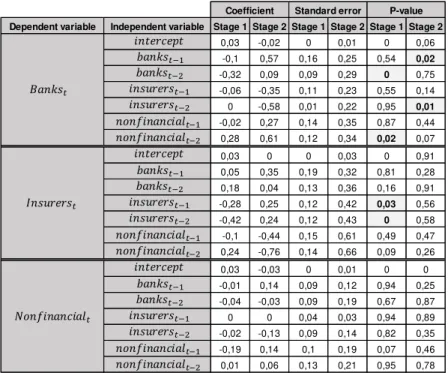
Table 5: Coefficients, Standard Errors and P-values of the Markov Switching Model
When analyzing the results of the Markov Switching Model, I conclude that there is
only indication of two interconnections among the sectors: in the stage of low volatility, the second lag of the non-financial companies’ past returns causes banks’ returns; in the
largest volatility regime, the second lag of the insurers’ past returns cause current banks’ returns. According to these results, within the “crisis” or high volatility regime, the
insurance companies’ past returns became more interconnected with the banking sector. The opposite is not verified, which emphasizes once more that the systemic importance of the insurers is not inferior when compared to the systemic importance of banks.
Dependent variable Independent variable Stage 1 Stage 2 Stage 1 Stage 2 Stage 1 Stage 2
0,03 -0,02 0 0,01 0 0,06 -0,1 0,57 0,16 0,25 0,54 0,02
-0,32 0,09 0,09 0,29 0 0,75 -0,06 -0,35 0,11 0,23 0,55 0,14 0 -0,58 0,01 0,22 0,95 0,01
-0,02 0,27 0,14 0,35 0,87 0,44 0,28 0,61 0,12 0,34 0,02 0,07
0,03 0 0 0,03 0 0,91
0,05 0,35 0,19 0,32 0,81 0,28 0,18 0,04 0,13 0,36 0,16 0,91 -0,28 0,25 0,12 0,42 0,03 0,56 -0,42 0,24 0,12 0,43 0 0,58 -0,1 -0,44 0,15 0,61 0,49 0,47 0,24 -0,76 0,14 0,66 0,09 0,26
0,03 -0,03 0 0,01 0 0
-0,01 0,14 0,09 0,12 0,94 0,25 -0,04 -0,03 0,09 0,19 0,67 0,87 0 0 0,04 0,03 0,94 0,89 -0,02 -0,13 0,09 0,14 0,82 0,35 -0,19 0,14 0,1 0,19 0,07 0,46 0,01 0,06 0,13 0,21 0,95 0,78
Coefficient Standard error P-value
𝑏𝑎𝑛𝑘𝑠𝑡−1 𝑏𝑎𝑛𝑘𝑠𝑡−2 𝑖𝑛𝑠𝑢𝑟𝑒𝑟𝑠𝑡−1 𝑖𝑛𝑠𝑢𝑟𝑒𝑟𝑠𝑡−2 𝑛𝑜𝑛𝑓𝑖𝑛𝑎𝑛𝑐𝑖𝑎 𝑡−1 𝑛𝑜𝑛𝑓𝑖𝑛𝑎𝑛𝑐𝑖𝑎 𝑡−2
𝑖𝑛𝑡𝑒𝑟𝑐𝑒𝑝𝑡 𝑏𝑎𝑛𝑘𝑠𝑡−1 𝑏𝑎𝑛𝑘𝑠𝑡−2 𝑖𝑛𝑠𝑢𝑟𝑒𝑟𝑠𝑡−1 𝑖𝑛𝑠𝑢𝑟𝑒𝑟𝑠𝑡−2 𝑛𝑜𝑛𝑓𝑖𝑛𝑎𝑛𝑐𝑖𝑎 𝑡−1 𝑛𝑜𝑛𝑓𝑖𝑛𝑎𝑛𝑐𝑖𝑎 𝑡−2 𝑖𝑛𝑡𝑒𝑟𝑐𝑒𝑝𝑡 𝑏𝑎𝑛𝑘𝑠𝑡−1 𝑏𝑎𝑛𝑘𝑠𝑡−2 𝑖𝑛𝑠𝑢𝑟𝑒𝑟𝑠𝑡−1 𝑖𝑛𝑠𝑢𝑟𝑒𝑟𝑠𝑡−2 𝑛𝑜𝑛𝑓𝑖𝑛𝑎𝑛𝑐𝑖𝑎 𝑡−1 𝑛𝑜𝑛𝑓𝑖𝑛𝑎𝑛𝑐𝑖𝑎 𝑡−2
𝑖𝑛𝑡𝑒𝑟𝑐𝑒𝑝𝑡 𝐵𝑎𝑛𝑘𝑠𝑡
𝐼𝑛𝑠𝑢𝑟𝑒𝑟𝑠𝑡
When comparing these results with the ones obtained from the VAR model, I
conclude that the number of statistically significant variables in the system has decreased.
5.4 Intra-Sector Interconnectedness of the Insurance Sector
When testing for the intra-sector interconnectedness, I had to once again divide my
data into two sub-periods: before and after the 2008 financial crisis. Due to the restricted number of observations, I have studied the number of interconnections only between 8
and 9 insurance companies before and after the crisis respectively. Again, I want to perform a Granger causality test to measure the interconnectedness, and the procedure described before was applied: I estimated a VAR model with all 8 (or 9) equations,
however as there was heteroscedasticity and autocorrelation, I have estimated the system using a GMM-HAC estimator in order to correct for both of these (Appendix 9). Below
in tables 6 and 7 one can see the p-values of these estimations.
Table 6: Pre-crisis coefficients of the VAR model estimated through the GMM-HAC method
Table 7: Post-crisis coefficients of the VAR model estimated through the GMM-HAC method
ALV GY CS FP ZURN VX SREN VX G IM MUV2 GY AGS BB AGN NA
-0.0079 -0.0014 0.0067 -0.0051 0.0024 -0.0060 0.0001 -0.0105
0.5211 0.6497** 0.6072** 0.4412* 0.1707 0.4887* 0.3715* 0.7209*
0.0810 -0.0322 0.2649 0.1980 -0.2006 0.0373 0.0156 0.1271
0.3260** 0.1798* 0.1668 0.1336 0.2887** 0.2593** 0.2467** 0.1413
0.2781 0.4551* 0.3883* 0.1941 0.3619* 0.6644 0.2168 0.3348
-0.5045 -0.1817 -0.0620 -0.3982** -0.1279 -0.5821 -0.2211 -0.4973 -0.4250* -0.5579** -0.4631 -0.4069 -0.1948 -0.5765** -0.2410 -0.5732
0.2671 -0.1453 0.096593 -0.0291 -0.0439 0.0462 0.0102 0.3446
-0.5392** -0.4717** -0.6644** -0.2251 -0.1886 -0.3941 -0.4324** -0.6452**
𝐿 𝑌𝑡−1 𝑁 𝑋𝑡−1 𝑆 𝐸𝑁 𝑋𝑡−1 𝐼 𝑡−1 2 𝑌𝑡−1
𝑆 𝐵𝐵𝑡−1 𝑁 𝑁 𝑡−1 𝐶𝑆 𝑃𝑡−1 𝐼𝑛𝑡𝑒𝑟𝑐𝑒𝑝𝑡
ALV GY CS FP ZURN VX G IM SREN VX MUV2 GY PRU LN TOP DC SAMPO FH
-0.0019 -0.0062 0.0029 -0.0115 -0.0005 0.0061 0.0029 0.0084 0.0121**
0.4020 0.4495* 0.2347 0.1489 -0.1861 -0.0313 0.6465** 0.1012 0.0857
-0.5333* -0.4910** -0.3052** -0.1527 -0.0797 0.0745 -0.5553** -0.2653** -0.0457
-0.1238 -0.1641 -0.0438 -0.0512 -0.0710 -0.0679 -0.1906 0.1251 0.0301
0.0057 -0.1305 0.0939 -0.2293* -0.2143 -0.0757 -0.0981 0.0206 -0.0354
0.1927 0.3324** 0.1948** 0.2299** 0.4074** 0.1181** 0.2538* 0.2481* 0.1293**
-0.2268 -0.4393** -0.3589** -0.3083 0.0958 -0.2314 -0.2719 -0.1139 -0.1413
0.0066 0.1483 0.0533 0.1287 0.1609 0.0142 -0.2486 0.0504 0.1041
0.0567 0.0386 -0.0263 0.0967 -0.1914 0.0644 0.2972* -0.1750 -0.0237
0.3879 0.4325 0.0996 0.0812 0.2698 0.0262 0.4166 0.0462 -0.1084
𝐼𝑛𝑡𝑒𝑟𝑐𝑒𝑝𝑡 𝐿 𝑌𝑡−1
𝐶𝑆 𝑃𝑡−1
𝑁 𝑋𝑡−1
𝐼 𝑡−1
𝑆 𝐸𝑁 𝑋𝑡−1
2 𝑌𝑡−1
𝑃 𝐿𝑁𝑡−1
𝑃 𝐶𝑡−1
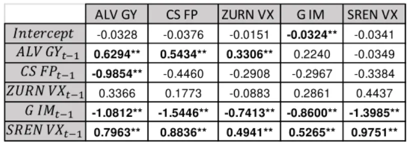
By analyzing the table below, one can conclude that the existing linkages between
the insurance companies are respectively 14 and 15 before and after the financial crisis at a 5% significance level. This seems to indicate that the panorama before and after the crisis is almost the same. However, when studying the existence of linkages during the
financial crisis (using only the 5 biggest companies in terms of average market cap at this time due to data shortage issues, and using data from January 2008 to June 2010), I
obtained the same 15 interconnections among insurance companies as can be seen below. This means that during the financial crisis, the interconnectedness among the insurance companies was larger than in the non-crisis period.
Table 8: Coefficients of the VAR model estimated through the GMM-HAC method (crisis period January 2008 to July 2010)
6. Conclusion
I have concluded that after the crisis the existing linkages between financial institutions and even between financial and non-financial institutions were larger than the
ones that existed before the crisis. Evidence suggests that only after the crisis do banks’ past returns Granger-cause the returns of the insurance companies and vice-versa.
Aside from this, I have split the non-financial industry in its components and concluded that the financial services industry also plays an important role as banks’ past returns Granger-cause its returns and financial services’ past returns itself Granger-cause
real estate returns. Among the non-financial industries, the telecommunications industry
ALV GY CS FP ZURN VX G IM SREN VX
-0.0328 -0.0376 -0.0151 -0.0324** -0.0341
0.6294** 0.5434** 0.3306** 0.2240 -0.0349
-0.9854** -0.4460 -0.2908 -0.2967 -0.3384
0.3366 0.1773 -0.0883 0.2861 0.4437
-1.0812** -1.5446** -0.7413** -0.8600** -1.3985** 0.7963** 0.8836** 0.4941** 0.5265** 0.9751**
𝐼𝑛𝑡𝑒𝑟𝑐𝑒𝑝𝑡 𝐿 𝑌𝑡−1
𝐶𝑆 𝑃𝑡−1
𝑁 𝑋𝑡−1
𝐼 𝑡−1
is the one that Granger-causes all other industries’ returns (including both financial and
non-financial companies).
When analyzing the intra-sector interconnectedness, I have concluded that the exiting linkages among insurance companies were more or less the same (and relatively small)
in the pre and post 2008 financial crisis periods. However when I isolated the crisis period and tested for the presence of interconnectedness, I concluded that in the crisis period the
number of interconnected insurance companies was much larger when compared to a non-crisis period.
It is of extreme importance to studying the systemic risk in the financial sector namely in the insurance sector and develop ways to measure the systemic risk and tools that allow to mitigate this risk.
By applying Granger causality tests one can conclude that before the financial crisis, there was no interconnection between banks and insurers returns, but that after the crisis,
banks past returns were able to explain (through a direct relationship) insurance companies current returns and vice-versa: there is after the crisis a feedback relationship between these two sectors.
The past long-term interest rate seems to be statistically significant to model the current insurers, banks and non-financial companies’ returns whereas the crude oil price
and the short-term interest rate seems not to be statistically significant. With respect to the Non-financial companies, those act as Granger receivers but they never Granger cause
other companies’ current returns.
5.
References
AASTVEIT, KNUT ARE. (2014). Oil price shocks in a data-rich environment. Energy
ACHARYA, VIRAL V.; LASSE HEJE PEDERSEN; THOMAS PHILIPPON; AND MATTHEW P.
RICHARDSON. (2010). Measuring Systemic Risk. Federal Reserve Bank of Cleveland
Working Paper 10-02.
ADRIAN,TOBIAS AND MARKUS K. BRUNNERMEIER. (2011). CoVar. National Bureau of
Economic Research Working Paper.
BIERTH,CHRISTOPHER;FELIX IRRESBERGER AND GREGOR N.F.WEIβ. (2015). Systemic
Risk of Insurers around the Globe. Journal of Banking & Finance, 55 (C): 232-245.
BILLIO,MONICA;MILA GETMANSKY;ANDREW W.LO AND LORIANA PELIZZON. (2012). Econometric Measures of Connectedness and Systemic Risk in the Finance and
Insurance Sectors. Journal of Financial Economics, 104 (3): 535-559.
BROOKS,CHRIS. Introductory Econometrics for Finance. (2008). Cambridge: Cambridge
University Press, 500-508
CHEN,HUA;J.DAVID CUMMINS;KRUPA S.VISWANATHAN; AND MARY A.WEISS.(2014). Systemic risk and the Interconnectedness between Banks and Insurers: An
Econometric Analysis. Journal of Risk and Insurance, 81 (3): 623-652
CUMMINS,J.DAVID AND MARY A.WEISS.(2014). Systemic Risk and the U.S. Insurance
Sector. Journal of Risk and Insurance, 81 (3): 489-528.
HAMILTON,JAMES D. (1983). Oil and the Macroeconomy since World War II. Journal of
Political Economy, 91 (2), pp. 228-248.
INTERNATIONAL ASSOCIATION OF INSURANCE SUPERVISORS (IAIS). (2011). Insurance
Core Principles, Standards, Guidance and Assessment Methodology. Basel: Bank for International Settlements.
INTERNATIONAL ASSOCIATION OF INSURANCE SUPERVISORS (IAIS). (2013). Global
Systemically Important Insurers: Initial Assessment Methodology.
JIMÉNEZ RODRÍGUEZ,REBECA AND MARCELO SÁNCHEZ. (2005). Oil price shocks and real
GDP growth: empirical evidence for some OECD countries. Applied Economics, 37
(2): 201-228.
NANDHA,MOHAN SINGH AND ROBERT FAFF. (2008). Does oil move equity prices? A
global view. Energy Economics, 30 (3): 986-997.
THE GENEVA ASSOCIATION. (2010). Systemic Risk in Insurance – An Analysis of
Insurance and Financial Stability, Special Report of the Geneva Association Systemic Risk Working Group, Geneva: The International Association for the Study of