Computational Techniques for Automated Analysis of Animal Tissue Histological Images

Faculdade de Engenharia da Universidade do Porto

Computational techniques for automated analysis of

animal tissue histological images

Frederico A. R. B. Junqueira

Master Thesis

Integrated Masters in Bioengineering

Supervisor:

Prof. João Manuel R. S. Tavares

Associate Professor of the Mechanical Engineering Department, FEUP

Co-Supervisor:

Augusto Manuel Rodrigues Faustino

Associate Professor of the Pathology and Molecular Immunology Department ICBAS

Agradecimentos

Em primeiro lugar quero agradecer ao Professor João Tavares pela disponibilidade e aconselhamento fornecidos ao longo destes últimos meses. Sem a sua orientação este trabalho não seria possível. Quero agradecer também ao Professor Augusto Faustino pela sua disponibilidade, simpatia e vontade de ajudar.

Quero agradecer do fundo do coração à Lia, que me acompanhou a 100% nesta jornada longa e nunca me deixou perder o Norte. Sem o seu carinho, muita paciência e apoio incondicional este trabalho não estaria completo.

À minha mãe, ao meu pai, à minha irmã, ao meu irmão e a minha avó pelas gargalhadas, carinho e todo o apoio nesta etapa final.

Ao Pedro pelos bons conselhos e ombro amigo sempre que precisei.

Ao companheiros da tese Morgana, Jessica e Ricardo por me ouvirem nos momentos de stress.

“Everybody has a plan until he gets punched in the face.” Myke Tyson

Resumo

O estudo de tecidos celulares fornece uma incontestável fonte de conhecimento e compreensão acerca do corpo humano e do ambiente que o rodeia. Aceder a esta informação é, portanto, crucial para determinar e diagnosticar uma grande variedade de patologias, detetáveis somente ao nível microscópico. A histologia desempenha um papel importante na observação de células e suas características anatómicas, e igualmente para o diagnóstico clínico de patologias involvendo uma anormal conformação celular. Nas imagens histológicas, algoritmos de segmentação semi-automáticos ou automáticos são capazes de separar e identificar estruturas celulares de acordo com as suas diferenças morfológicas. Estes algoritmos de segmentação são a primeira abordagem a sistemas de visão computacional e, no que respeita à histopatologia, o diagnóstico automático de imagens histológicas. Como as amostras histológicas têm uma espessura reduzida, as características volumétricas são quase imperceptíveis, correespondendo a perdas de informação valiosas, principalmente topográficas e volumétricas, críticas para um correcto diagnóstico.

Consequentemente, a combinação de algoritmos de segmentação e reconstrução 3D aplicados a datasets de imagens histológicas fornecem uma maior informação acerca da patologia analisada e estruturas microscópicas, destacando regiões anormais.

Tendo isto em consideração, o presente trabalho focou-se em desenvolver algoritmo computacional automático capaz de realizar reconstrução 3D de superfícies de tecidos relevantes em secções histológicas 2D. Uma primeira abordagem foi desenvolvida focada em destacar as estruturas relevantes nas secções de tecido. Depois, um estudo feito com base em algoritmos de registo de imagem foi levado a cabo para descobrir qual a metodologia mais indicada para alinhar as secções provenientes de datasets de imagens. Combinando os melhores métodos de processamento e registo de imagem (resultado DICE para caso 1: ; resultado DICE para caso 2: ; resultado DICE para caso 3: ), avaliados em abordagens prévias, em conjunto com um algoritmo de reconstrução 3D foi possível uma representação volumétrica das estruturas de tecidos pertinentes do dataset de imagens alinhadas.

Abstract

The study of cellular tissues provides an incontestable source of information and comprehension about the human body and the surrounding environment. Accessing this information is, therefore, crucial to determine and diagnose a wide variety of pathologies detectable only at a microscopic scale. Histology plays an important role in the observation of cells and their anatomical features, and so for clinical diagnosis of all the pathologies involving abnormal cellular conformation. In the histological images, semi-automated or automated segmentation algorithms are able to separate and identify cellular structures according to morphological differences. These segmentation algorithms are the first approach for computational vision systems and, concerning histopathology, the automated diagnose of histological images. Since the histological samples are thin, the volumetric features are almost unnoticeable, corresponding to losses of valuable information, mainly topographical and volumetric data, critical for a correct diagnostic.

Hence, the combination of segmentation and 3D reconstruction algorithms applied to histological image datasets provides more information about the analysed pathology and microscopic structures, highlighting abnormal areas.

Taking this into consideration, the present work focussed on developing an automatic computational algorithm capable of performing the 3D surface reconstruction of relevant tissue structures of 2D histological slices. A first approach was developed fixed on highlighting the relevant structures from the tissue sections. After that, a study on image registration algorithms was conducted to find the most suited methodology to align the slices from histological image datasets. Combining the top-performing image processing and registration methods (DICE score: 0.9267±0.0337 for Case 1; 0.9367±0.0356 for Case 2; 0.9683±0.0283 for Case 3), evaluated in the previous approaches, with a 3D surface reconstruction algorithm it was possible to calculate a volumetric representation of the pertinent tissue structures from the aligned image dataset.

Contents

Chapter 1 ... 1

Introduction ... 1

Chapter 2 ... 5

Literature Review ... 5

2.1.3. Microscopy and Histological Sample Observation ... 12

2.2. Image Processing ... 17

2.2.1. Image Pre-Processing ... 18

2.2.2. Image Segmentation ... 22

2.3. Image Registration and 3D Reconstruction ... 25

2.4. Key Issues ... 35

Chapter 3 ... 37

Methodology ... 37

3.1. Dataset ... 37

3.1.1. Tissue Sample Preparation and Digital Image Acquisition ... 38

3.1.2. Tissue Analysis and Image Datasets ... 38

3.2. Workflow implementation ... 41

3.2.1. First Approach – Based on pre-processing and Segmentation ... 41

3.2.2. Second Approach – Based on Image Registration ... 45

3.2.3. Final Approach – Based on the complete workflow with the 3D reconstruction . 48

Chapter 4 ... 53

Results and Discussion ... 53

4.1. Pre-processing stage ... 53

4.2. Registration stage ... 66

Conclusion... 83

5.1. Future Work Perspectives ... 84

List of Figures

Figure 1. Epithelial tissue classification according to the number of cell layers and cellular

shape. ... 7

Figure 2. Representative images from adult loose connective tissue (left) and adult dense connective tissue (right). ... 8

Figure 3. Histological image showing a transverse section of skeletal muscle. ... 9

Figure 4. Histological image showing cardiac muscle. ... 9

Figure 5. Histological image from a section of smooth muscle. ... 10

Figure 6. Histological image showing a section from cerebral cortex, stained with Golgi-Cox method (stains neurons in black). ... 10

Figure 7. Histology picture of a set of cells lining a duct stained with H & E (on the left), and a histology image stained with immunohistochemical techniques to enhance, in red, the presence of the protein actin in the cells (on the right). ... 12

Figure 8. Comparative images acquired from optical microscopy (a) and electron microscopy (b). ... 14

Figure 9. Leeds University wall-sized virtual microscope. ... 15

Figure 10. Sequence of histological images from MKI (Mitosis-karyorrhexis index) cells, varying in color information due to staining differences. ... 20

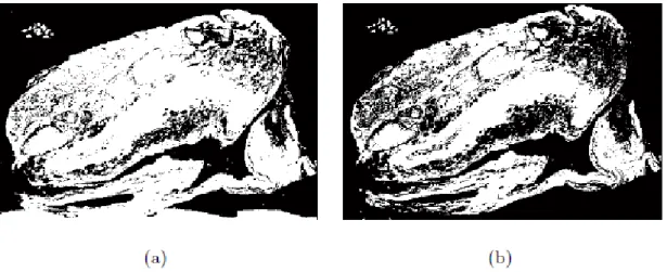
Figure 11: Relevant tissue structure segmented using (a) the global thresholding approach and (b) k-means algorithm. ... 25

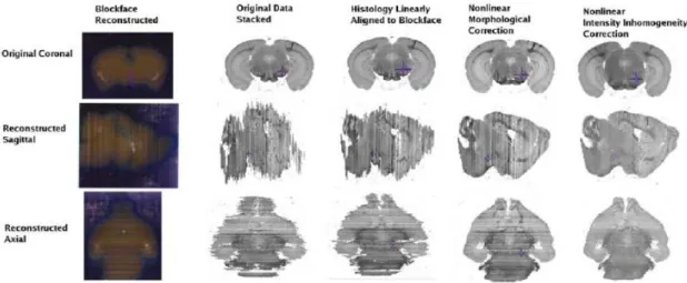
Figure 12. Image from an example of blockface used for 3D reconstruction. ... 26

Figure 13. Two views of 3D reconstruction of uterine cervix carcinoma tumor invasion fronts, from different histological specimens. ... 28

Figure 14. 3D reconstruction of invasive breast carcinoma immunohistochemically stained, illustrating the spatial arrangement of the different parenchymal tissues. ... 29

Figure 15. Volumetric results from the reconstruction of serial histological slices acquired by Chakravarty M. and collaborators. ... 32

optimizer (B,D) on 2 slides from placenta image dataset (PCA was applied initially as pre-processing). ... 33 Figure 18. Image from Case 1 (Slice nº 51) – Testicular tissue section with a collision

tumor (A). Epididymis is (B) and Connective tissue (C). ... 39 Figure 19. Image from Case 2 (Slice nº 5) – Lymph node tissue section with a possible

neoplasic region (A). A blood vessel is marked by (B). ... 39 Figure 20. Image from Case 3 (Slice nº 33) – Lymph node tissue section with neoplasic

regions (A) and (B). Blood vessels are marked by (C). ... 40 Figure 21. Image removed from case 2, due to presence of folds on the tissue section,

produced in the mounting process. ... 41 Figure 22. Schematic model representing the first workflow implemented in the study. ... 44 Figure 23. Representation of the intensity-based registration framework implemented. ... 46 Figure 24. Schematic model representing the second workflow implemented in the study. .. 48 Figure 25. Schematic model representing the third and final workflow implemented in the

study. ... 51 Figure 26. Original image (slice nº35) from the second dataset. ... 54

Figure 27. Resultant images of color channel extraction from the original image. Red

channel grayscale image – R, Green channel image – G and Blue channel image – B. .... 54 Figure 28. Images obtained through CLAHE implementation on the original RGB image

channels. ... 55 Figure 29. RGB image obtained after CLAHE operation in each color channel image from

the original image and posterior concatenation of the channels (a). RGB image obtained after CLAHE-red operation in the red channel and posterior concatenation with unaltered green and blue channels (b). ... 56 Figure 30. Normalized RGB image resultant from the Normalization technique described in

section 3.2.1. ... 57 Figure 31. Images resultant of the normalization procedure to each color channel (Red –

R, Green – G and Blue – B). ... 57 Figure 32. Images obtained with HSV color transformation with four different saturation

enhancement factors, from the original image. ... 58 Figure 33. Image obtained through CIE L*a*b color space transformation, from the original

image. ... 59 Figure 35. Resultant images from YCbCr color space transformation applied to the

normalized RGB image (Figure 30). ... 60 Figure 36. Mask structure, created from the original image to remove the background (a). .. 61

Figure 38. Segmentation results considering four classes, for CLAHE image (a), HSV

enhanced image (b), L*a*b transformed image (c) and YCbCr image (d). ... 63 Figure 39. Original image (slice nº 35) from case 1 (on the left). Original image (slice

nº35) from the third dataset (on the right). ... 63 Figure 40. Masked images, resultant from the contrast enhancement techniques applied

to the original image from case 1 – CLAHE-red (a), YCbCr (c). ... 64 Figure 41. Masked images, resultant from the contrast enhancement techniques applied

to the original image from case 3 – CLAHE-red (a) and YCbCr (c). ... 64 Figure 42. Images representing intensity-based image registration performed with

reference slice model and two types of transformation, from YCbCr pre-processing. ... 68 Figure 43. Images representing intensity-based image registration pairwise model and

rigid transformation type, from YCbCr pre-processing. ... 68 Figure 44. Images representing intensity-based image registration performed with

reference slice model and rigid transformation type, from CLAHE-red pre-processing. . 69 Figure 45. Images representing intensity-based image registration performed with

pairwise model and similarity transformation type, from smoothed image

normalization pre-processing. ... 70 Figure 46. Images representing the intensity-based non-rigid registration. ... 72 Figure 47. Illustrative images presenting a distortion error in the registration. ... 72 Figure 48. Images representing intensity-based image registration performed with

reference slice model and rigid transformation type, from CLAHE-red pre-processing. . 74 Figure 49. Images obtained from the combined pre-processing framework YCbCr

luminance enhancement and CLAHE-red applied to the original images. ... 75 Figure 50. Segmentation results obtained with the stain deconvolution algorithm (first

column): case 1-(a), 2-(d) and 3 (g). ... 76 Figure 51. Images representing intensity-based image registration performed with

reference slice model and rigid transformation type, from hematoxylin images

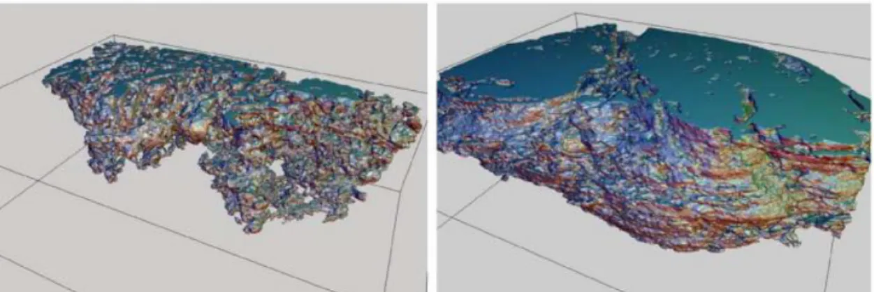
obtained through stain deconvolution (Case 3). ... 77 Figure 52. 3D surface reconstruction from case 3 registered image dataset, using Marching

cubes algorithm. ... 78 Figure 53. 3D surface reconstruction from case 2 (second line) and 3 (first line) registered

List of Tables

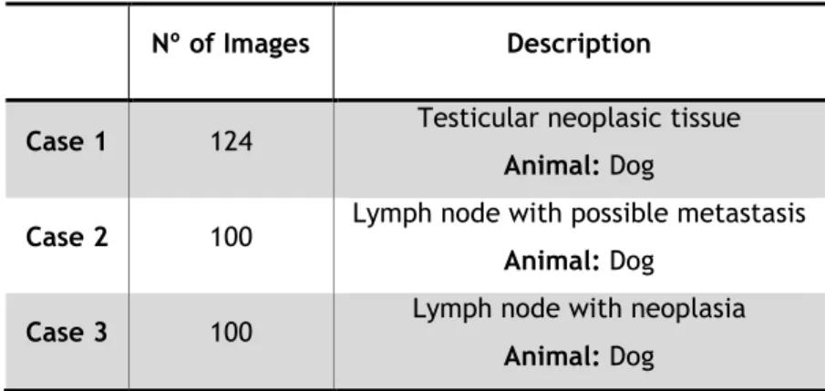
Table I. Characterization of the three image datasets studied in this work. ... 38 Table II. Table containing the mean DICE scores and the elapsed times for the

intensity-based registration implementation, with different types of transformation (rigid, similarity and affine) and models (reference slice, pairwise), on images from both top-performing pre-processing methods (YCbCr color transformation and

CLAHE-red). ... 66 Table III. Table containing the mean DICE scores and the elapsed times for the

feature-based registration implementation with pairwise model on images with both

smoothed and non-smoothed image normalization pre-processing. ... 69 Table IV. Table containing the mean DICE scores and the elapsed times for the

intensity-based non-rigid registration implementation, with two different algorithms (B-spline and Demon) and models (reference slice, pairwise), on images obtained from CLAHE-red pre-processing method. ... 71 Table V. Table containing the mean DICE scores and the elapsed times for the

intensity-based rigid registration method implementation, on two different image datasets (Case 1 and 2), previously pre-processed by CLAHE-red algorithm. ... 73 Table VI. Table containing the mean DICE scores and the elapsed times for the

intensity-based rigid registration method implementation, on all the image datasets (Case 1, 2 and 3), considering two different grayscale images (hematoxylin and eosin images), obtained through pre-processing (CLAHE-red and YCbCr transformation) and

Abbreviations and Acronyms

CNS Central Nervous System

CT Computer Tomography

ECM Extracellular Matrix H & E Haematoxylin and Eosin HSV Hue – Saturation - Value

ITK Insight Segmentation and Registration Toolkit

µm Micrometer

mm Millimeter

MRI Magnetic Resonance Imaging

nm Nanometer

PCA Principal Component analysis PET Positron Emission Tomography PNS Peripheral Nervous System

3D Three Dimensions

2D Two Dimensions

RGB Red – Green - Blue

CLAHE Contrast Limited Adaptive Histogram Equalization

Introduction

1.1 - Motivation

Histological studies provide an important help in the understanding of some complex pathophysiological processes concerning diseases at the cellular scale. These studies are considered the gold standard for assessing the natural response of a cellular tissue in face of a pathology or therapeutic intervention (Chakravarty, Bedell et al. 2008). To produce histopathology slides, a rather complex protocol must be executed involving a substantial amount of human labor and information processing (Randell, Ruddle et al. 2012).

Although in-vivo imaging techniques, such as the MRI and PET, assess anatomical and pathological information without invasive procedures, they require extensive validation when compared to histological ex-vivo examinations (Chakravarty, Bedell et al. 2008).

Visual interpretation, the core of most medical diagnostic procedures and the final diagnostic decision for cancer and other diseases, is based on tissue examination. This method requires a long time, intensive manual labor to produce viable results and presents a sampling bias that promotes intra- and inter-reviewer discrepancies when analysing histological tissues (Sertel, Kong et al. 2009). Thus, it is clear the need for automated processes concerning morphology diagnostics in medicine, to improve the diagnostic accuracy and provide a fast and reliable second opinion to histopathologists. Automated systems can reduce human factor mistakes and increase the speed of diagnostic processes (Nedzved, Belotserkovsky et al. 2005).

The volumetric data analysis from relevant tissue structures visible from 2D histological slices is not often a straightforward process, requiring a great amount of experience from histopathologists (Koshi, Holla et al. 1997). Therefore, three dimensional reconstruction of tissue samples at a microscopic resolution reveals significant potential to improve the study of

disease processes when structural or spatial modifications are involved (D. 1978). The combination of 3D image reconstruction methodologies with staining techniques provides a better understanding on functional information concerning the cellular structures (Roberts, Magee et al. 2012).

Hence, there is an urge to develop fully automated approaches for tissue analysis in histological section images, combining the best computational methods to produce an accurate and reliable 3D reconstruction algorithm, enhancing this way the medical study and clinical diagnostic of various diseases. The implementation of these algorithms could provide a better insight into the intricate spatial relations between the studied cell tissues and surrounding tissues.

With this in mind, a computational framework was developed in this study, composed by several image processing and registration algorithms and culminating in a 3D tissue reconstruction method. To accomplish this, a previous literature review was performed on the most suited methods to perform each task, as well as histological image notions, crucial to correctly analyse the image datasets tested to validate the developed algorithm, and also to define the relevant tissue structure to be reconstructed.

1.2 - Objectives

The present study aimed, primarily, the review and evaluation of currently implemented image processing and registration techniques in the literature, ranging from standard pre-processing methods to complex image registration frameworks, and recently developed algorithms for histological image analysis.

With all the concepts and information gathered from the literature review, it was possible to pursue the main goal of this study, which consisted in the development of a completely automatic computational framework, capable of performing accurate histological image alignment and 3D reconstruction of tissues. Therefore, providing detailed volumetric information concerning relevant tissues features, unobtainable through 2D conventional slice analysis. The objectives behind each step developed for the final framework, are explained below.

Image pre-processing – first step, developed to accomplish the highest color differentiation between tissues with distinct stains, with several contrast enhancement methods being tested.

Image segmentation – aiming to provide the most accurate discrimination between different tissue stains and/or other interesting structures in the histological images, previously pre-processed.

Image registration – for the implementation of this step, the great focus was to achieve the most correct slice alignment, thus, mimicking the original disposition of histological tissues in natural conditions, before the tissue preparation procedure.

with this step is to provide detailed three dimensional insight over commonly studied 2D tissue structures, such as neoplasic tissues.

1.3 - Document Structure

The present work is divided in 4 chapters, besides the introduction. A brief description on the contents and subjects addressed in each one is provided below.

Chapter 2 - Literature Review: On this chapter, an introduction to histology and its

importance as a way to assess cellular responses to pathogens or treatments at a microscopic level is addressed, as well as the standard histological tissue sample preparation, for microscopic observation. This last topic is also discussed, including standard and recent techniques to perform microscopic observation on histological tissue sections. In this chapter, it is also presented a review on both standard and recently developed image processing methods, including pre-processing techniques, segmentation methods and registration algorithms, implemented on stained histological images.

Chapter 3 – Methodology: This chapter describes the implemented methodology in this

project, approaching first the pre-processing techniques tested, followed by image registration frameworks and culminating in the final workflow. The histological image dataset used to test the developed computational framework is also described in this chapter.

Chapter 4 – Results and Discussion: In this chapter, all the results obtained either from

pre-processing methods, segmentation or registration methodologies are presented and systematically discussed.

Chapter 5 – Conclusion: This last chapter, comprehends the final conclusions about the

results, obtained through the performed study, in addition to future development perspectives.

1.4 - Principal Contributions

The principal contributions provided by the present work can be subdivided into two domains: the literature review and the developed computational framework.

The literature review presented represents an introduction to researchers or developers interested and unfamiliar with histological tissue image processing methods, to fundamental

histology concepts as well as computational techniques, ranging from image pre-processing to image registration algorithms, suited for histological tissue samples. Furthermore, it also presents current state of the art methodologies for image registration, implemented in histological image datasets, which obtained successful slice alignment results.

The pre-processing preliminary evaluation on color space transformation methods, best suited to enhance color contrast in stained tissue images, is complete and the resultant image examples presented in this document provide a great insight on these simple algorithms to increase RGB color contrast, not only applicable to histological slices. The CLAHE-red technique was conceived for the present work, and it was proven to be the best pre-processing method to enhance stain contrast in H & E histological images, originating accurate tissue segmentation results, with simple clustering methods (kmeans).

The stain deconvolution algorithm, despite being based on previous works on the literature, the computational framework that enabled automatic stain discrimination was conceived and developed in this project. This was accomplished using simple techniques and the results obtained were consistent for most of the tested histology slices.

The entire computational framework proposed in this project enables the reconstruction of a three dimensional volume based on real histological tissue structures. It was achieved through the implementation of computationally cheap algorithms, and were obtained highly detailed volumetric representation, not only of differently stained tissues but also, in some cases, the accurate reconstruction of neoplasic tissues, present in the considered histological image datasets.

Literature Review

This chapter presents the essential concepts required to understand the topics under study as well as all the research done so far on the subject.

Firstly, it will be presented an overview on the histological concepts concerning the current laboratory approach for acquisition of samples, as well as the relevant features of the different types of cellular tissues, since these images from the tissue samples represent the case study of this project.

A study on the most suitable computational methods to process and extract information from the histological images is reviewed and analyzed further in this chapter. This literature review culminates in the presentation and analysis of the most accurate 3D reconstruction algorithms for biological images, regarding the future reconstruction of certain relevant portions of cellular tissues in the histological samples.

2.1. Histology

Histology is the science that is devoted to study the detailed morphology of cells and tissues concerning the way in which these constitute the different organs in the body, at a microscopic level. The methods implemented by histologists require the study of living cells outside the conditions in which their development is natural, imposing a controlled environment (Junqueira and Carneiro 1987).

Histological studies provide an important help in the understanding of some complex pathophysiological processes concerning diseases at the cellular scale. Since these studies are also fundamental to evaluate the performance of new therapies and drug agents, they are considered the gold standard for assessing the natural response of a cellular tissue in face of a

pathology or therapeutic intervention (Chakravarty, Bedell et al. 2008). The histological investigation, or the analysis of cell structures and tissues of different parts of the human body, is the focus of medical morphology, which is considered the most decisive method in the diagnostic of several human diseases (Nedzved, Belotserkovsky et al. 2005). Histopathologists can diagnose cancer and other pathologies through the observation under the microscope of sections of human or animal tissues (Randell, Ruddle et al. 2012). This histopathological diagnostic can be attained, for example, through the knowledge of some particular histological patterns, visible at the microscope, that are specific for a certain tumour or group of tumours, thus helping to provide and deliver the adequate treatment (Dive, Bodhade et al. 2014).

Considering that histological studies require biopsies or ex-vivo models, considering animal examinations (impossible to perform in live specimens), to assess disease and therapeutic efficiency tests results, these methods present serious disadvantages when compared to powerful imaging methods, such as high-resolution magnetic resonance imaging (MRI) and positron emission tomography (PET) scanners that are non-invasive and can be performed in in-vivo models, enabling longitudinal studies of the same specimen. Despite these advantages, the last methods require an extensive validation when compared to the gold-standard ex-vivo methods (histological observations) (Chakravarty, Bedell et al. 2008), highlighting the relevance of the histological methods nowadays.

Further in this section, the fundaments of histology are introduced and the procedure involved in the production of tissue samples for microscopic observation, as well as the different tissue types existent in the human body are explained.

2.1.1. Tissue Types

All tissues share the same basic biological components, cells and extracellular matrix (ECM). The latter is constituted by a complex and deeply organized network of biomolecules that surrounds the cells forming an intensive connection, in order to grant and supply all the necessary nutrients and molecules demanded by the organism (Junqueira and Carneiro 1987).

The human body is composed by four principal types of cellular tissues, the epithelial tissue, the connective tissue, the muscle and the nervous tissue. The functional, structural, molecular and visual characteristics of these four types of tissue are explored bellow.

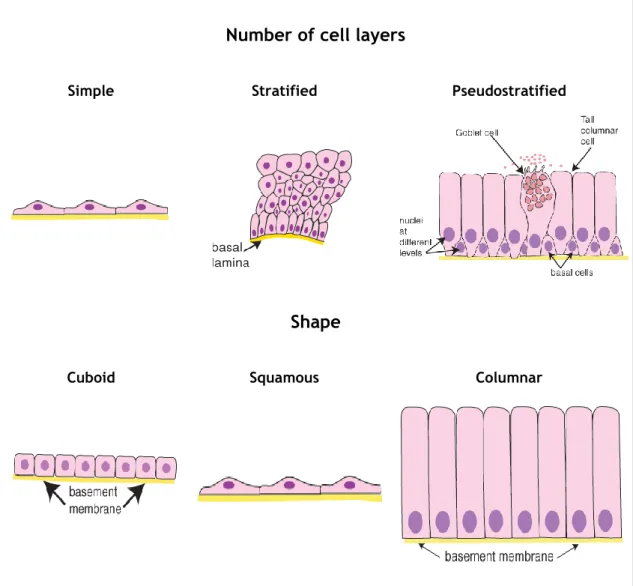
Epithelial tissue is formed by tightly united sections of cells that cover all body surfaces,

such as skin and intestine (except the articular cartilage), and represent the functional units of secretory glands. The epithelium presents a reduced amount of ECM and it stands over a basement membrane, a thin layer of specialized ECM that supports the epithelial structure providing mechanical bracing, attachment site and acts as a selective filtration barrier. The epithelial tissue can be classified in three main categories according to the number of cell layers that compose the tissue. Simple epithelia is formed by one layer of cells and the Stratified epithelia by two or more layers of cells. The third type is the Pseudostratified

epithelia that, despite being also composed by one layer, not all the cells contact with the epithelium’s surface resulting in an irregular distribution of the cell’s nucleus. These categories can be subdivided, based on the shape of the cells present in the surface layer in squamous, cuboid and columnar (note: epithelia is the plural form of epithelium) (Junqueira and Carneiro 1987, Paulsson 1992, Kierszenbaum 2007). Figure 1 illustrates the different categories of epithelial tissue.

Number of cell layers

Simple Stratified Pseudostratified

Shape

Cuboid Squamous Columnar

Figure 1. Epithelial tissue classification according to the number of cell layers and cellular shape. Adapted

from Leeds University Histology Guide (Michelle Peckham 2003).

Connective tissue is responsible for providing a support and connection structure for all

other tissues and cells of the body, contributing to its shape maintenance. The connective tissue is formed by ECM and cells but, unlike the epithelium, the intercellular distance is greater, due to the large presence of ECM components in tissue, surrounding the cells. Concerning the extracellular matrix composition, it is a combination of a large number of biomolecules, namely collagen (the most abundant), elastin (provides elastic resilience to the

connective tissue), fibronectin with the role of matrix’s structure organizer, glycoproteins and proteoglycans (Kierszenbaum 2007, Halper and Kjaer 2014).

The connective tissue can be classified in embryonic, adult and specialized connective tissue. The embryonic tissue is an unconstrained tissue developed during early embryonic stages, present in the umbilical cord. Adult connective tissue comprises a large diversity of structures due to the variable cell-to-ECM ratio, therefore leading to the subdivision in two types of tissue, the loose and the dense connective tissue. Loose tissue exhibits more cells than collagen fibers, and it is mainly present in the vicinity of nerves, blood vessels and muscles. On the other hand, the dense connective tissue is richer in ECM fibers, and it is present in tendons, ligaments and the dermis (skin). Specialized connective tissue includes tissues with special properties such as the adipose tissue, cartilage, bone and bone marrow tissue (Kierszenbaum 2007).

Examples of the abovementioned adult connective tissues can be visualized in Figure 2.

Muscle tissue consists of elongated cells, the myofibers, especially designed for

contraction, which is promoted by the mechanical energy produced in the cells. The cellular membrane of muscle cells is the sarcolemma and the cytosol is denominated sarcoplasm.

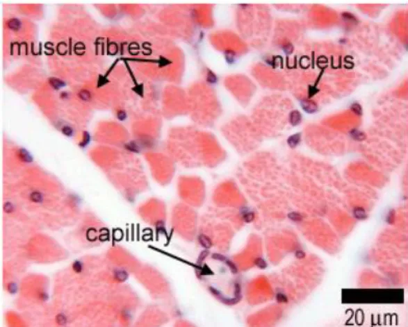
The muscle tissue is divided in three types: skeletal, cardiac and smooth muscles. The skeletal muscle is composed of bundles of long, cylindrical and multinucleated cells exhibiting transverse striations. This muscle tissue contract voluntarily in a fast and vigorous way. In the skeletal muscle fibers, the various nucleus are located in the peripheral part, a distinguishing factor when comparing to the cardiac muscles. The cardiac muscle cells present transverse striations, one or two centered nucleus as well as an elongated and ramified shape. These cells are united by intercalated disks and exhibit involuntary, vigorous and rhythmic contraction. The cardiac fibers are surrounded by a sheath of connective tissue that assures the muscle with a wide capillary network. The smooth muscle is originated from the aggregation of long cells,

Figure 2. Representative images from adult loose connective tissue (left) and adult dense

connective tissue (right). Adapted from Leeds University Histology Guide (Michelle Peckham 2003).

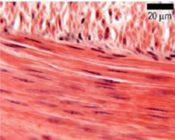
thicker in the center. This muscle tissue is coated by a basement membrane and structurally supported by a set of reticular fibers, enabling the simultaneous contraction of the entire muscle (Junqueira and Carneiro 1987, Kierszenbaum 2007). Illustrative images on the several types of muscles are shown in Figure 3, 4 and 5.

Figure 3. Histological image showing a

transverse section of skeletal muscle. Adapted from Leeds University Histology Guide (Michelle Peckham 2003).

Figure 4. Histological image showing cardiac

muscle. Adapted from Leeds University Histology Guide (Michelle Peckham 2003).

Figure 5. Histological image from a section of

smooth muscle. Adapted from Leeds University Histology Guide (Michelle Peckham 2003).

Nervous tissue interconnects itself in the body to create a network, the nervous system,

which is divided into two subsystems, the central nervous system (CNS) and the peripheral nervous system (PNS). The brain and spinal cord are the major components of the CNS while the PNS comprises the nerves (extensions of the neurons, nervous cells) and peripheral ganglia, establishing the connection with the CNS. The nervous system is responsible for the detection of sensorial stimuli from the exterior environment, integration of the received sensorial information, coordination of vital functions in the body and transmission of motor stimulus to the muscles (Junqueira and Carneiro 1987, Kierszenbaum 2007).

The nervous tissue in the CNS is the combination of neurons and glial cells, the latter ensuring structural support and correct conditions in the neurons’ membrane for the transmission of electric signals. In the CNS there is a separation between the neurons’ cellular body and their extensions, corresponding to two visually distinct sections, the gray matter and the white matter (both sections contain glial cells) (Junqueira and Carneiro 1987). A histological sample of nervous tissue illustrating both white and grey matter is shown in Figure 6.

Figure 6. Histological image showing a

section from cerebral cortex, stained with Golgi-Cox method (stains neurons in black). Adapted from Leeds University Histology Guide (Michelle Peckham 2003).

2.1.2. Sample Preparation

Considering that histology is the visualization of cells under the microscope, certain procedures must be performed in order to obtain thin tissue samples (slides) of the organ or biological structure under study. The process to study cellular tissues at the optical microscope (described in more detail in section 2.1.3) consists in the preparation of histological sections or slides (Junqueira and Carneiro 1987). To produce these slides, a rather complex protocol must be executed involving a substantial amount of human labor and information processing (Randell, Ruddle et al. 2012).

The specimens for analysis can range from small pieces of tissue collected from biopsies to entire organs. Most of these specimens are thick and cannot be traversed by light, thus justifying the slicing in thinner portions. The production process of glass slides consists, first, of a dissection step to, as already said, obtain tissue portions where the disease or area of interest is macroscopically located. Then, these tissue sections are chemically processed in a fixation step, followed by an inclusion procedure and after this, a new cut in the tissue block is performed using a microtome, a high precision cutting device, to obtain the final glass slice thickness (5 µm). An important staining procedure is performed finally in the tissue slides to increase the contrast of certain cellular structures (Junqueira and Carneiro 1987, Randell, Ruddle et al. 2012). A more detailed explanation on the fixation, inclusion and staining processes is presented below.

 Fixation – the purpose of this process is to toughen and preserve the microstructure

and molecular composition of the tissue, thus avoiding the enzymatic and bacterial digestion. The fixation process involves the immersion of the tissue sample in a denaturizing and stabilizing solution, which diffuses itself and penetrates into the interior of the sample. The most widely used fixation agent for observation in optical microscopy is a solution of formaldehyde at 4% (Junqueira and Carneiro 1987).

 Inclusion – In order to obtain thin sections for microscope observation using the

microtome, as stated, the previously fixated tissue samples must be embedded in paraffin (optical microscopy), or certain plastic resins (optical and electronic microscopy), to provide them a more rigid complexion. The inclusion step is often preceded by a dehydration and clearing steps to supplant the water present in the tissues by alcohol and then, the latter by xylene (paraffin is soluble in xylene) (Junqueira and Carneiro 1987). An alternative approach for this method that replaces both described fixation and inclusion steps is the frozen fixation, further described in this section.

 Staining – Considering that one or more sections sliced from the tissue block may be

placed on a single slide or several slides for comparison, they can be stained with a wide variety of chemical or immunologically based procedures. The staining methods selectively highlight several components in the tissues, cells and ECM. The prevalent staining technique is the haematoxylin and eosin method (H & E), capable of

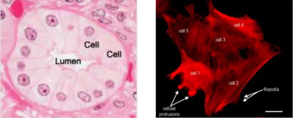
highlighting most of the significant cellular structures in the tissues. This technique stains the cell nucleus and other acidic structures in blue or violet (haematoxylin) and in pink the cytoplasm and collagen (eosin). Other techniques enable the contrast of more specific tissue structures or organisms by recurring to histochemical reactions, and also, in the case of immunohistochemical stains, to assess the presence or absence of a certain protein. These methods are performed only when the H & E staining fails to accentuate the contrast of the studied structure in the tissue (Junqueira and Carneiro 1987, Randell, Ruddle et al. 2012). Representative images of the visual appearance under the microscope of the referred staining methods applied on cellular tissues are presented in Figure 7.

Figure 7. Histology picture of a set of cells lining a duct stained with H & E (on

the left), and a histology image stained with immunohistochemical techniques to enhance, in red, the presence of the protein actin in the cells (on the right). Adapted from Leeds University Histology Guide (Michelle Peckham 2003).

In the frozen fixation, the tissues to be analysed are rapidly frozen (replacing the chemical fixation and inclusion steps in the previous protocol), and then stained with H & E technique. Despite producing lower quality slides this method acquires slices in a shorter time, ideal when is required a fast examination of the tissue (Randell, Ruddle et al. 2012).

2.1.3. Microscopy and Histological Sample Observation

After the preparation of histological samples (more details in section 2.1.2) the microscopic cellular structures present in them are observed under the microscope. In this section, the prevalent types of microscopy implemented to visualize and analyze those tissue slices as well as innovative methods to perform the observation and diagnostic of histological images are addressed. There are two major types of microscopy devices, the light or optical microscopes and the electronic microscopes. The most critical factor concerning a microscope is its resolution power or resolution limit, which is measured by the minimum distance between two particles in the image (Junqueira and Carneiro 1987, Randell, Ruddle et al. 2012). Functional and operational details concerning different microscopes of both groups are explained further.

The conventional light or optical microscope exhibits images of the stained tissues through illumination, which transverses the sample, generated by a light source. It is composed by both mechanical and optical parts and has a limit resolution of 0.2 µm. The optical part comprises three sets of lenses, namely the condenser, the objectives and ocular lenses. The first condenses the light from the source to the histological sample, the objectives collect the light that crossed the sample and projects an augmented version of the received image, ranging the magnification from 2.5x to 40x, into the ocular lens also contributing for the final magnification in a factor of 10. The final magnification is then, the product of both objective and ocular magnification. However, by convention the ocular magnification factor is not included in image descriptions. Besides the normal light microscope, optical microscopy also comprises other two major types of microscopes, the confocal and the fluorescence microscopes (Junqueira and Carneiro 1987, Randell, Ruddle et al. 2012).

Confocal microscopes allow the focusing of thinner sections in the image, avoiding the

observation of overlapping planes of the tissue, fact that degrades and reduces the image’s definition. In order to perform this specific focus, the light beam that crosses the histological sample is narrow and the tissue’s image must transverse a small orifice. Consequently, this setup only allows the focussed plane of the original image to reach the detector, blocking all other consecutive planes. Since only a thin section is focussed at a time it is possible the three dimensional (3D) reconstruction by gathering all the planes of the analyzed tissue, through a computational algorithm (application later explored in the following sections) (Junqueira and Carneiro 1987).

In fluorescence microscopy, the analyzed samples are lighted by a mercury light source and, by recurring to certain filters the wave-length of the projected light can be regulated. Certain biological structures present in the tissue sample have affinity to fluorescent substances that when excited by the projected light they answer by emitting light in specific wave-length. Through the application of this technique certain biological components exhibit bright colors in the observed image, being highlighted from the surroundings (Junqueira and Carneiro 1987).

Electronic microscopy is based on the interaction between electrons and the tissues

present in the sample to be analyzed. Considering that light microscopes have a limit resolution of 0.2 µm, electron microscopy represents a more accurate solution, offering a more detailed image of smaller components in the studied tissue with a limit resolution of approximately 3 nm. Nowadays, exist two types of electron microscopes, transmission and scanning electron microscopes (Junqueira and Carneiro 1987).

Transmission microscopes possess a resolving power of approximately 3 nm, thus allowing

the detailed observation of isolated biomolecules or particles 400 thousand times magnified. For entire tissue samples, the magnifying power is reduced to 120 thousand times, still a high resolution when compared with the optical microscope. The operating mode of this microscope is based on the detour of electrons when in contact with magnetic fields analogous to lens’

light reflection in the optical microscope. The electron beam is produced upon heating a tungsten cathode, and, due to a voltage potential between the latter and the anode, the electrons are accelerated and transverse in high speed the microscope tube. In the tube, the beam is condensed through an electromagnetic lens (coils) and interacts with the tissue sample, traversing it and being consecutively amplified by a sequence of magnifying lenses. In the end, the electrons reach a detector (fluorescence plate) and imprint a black and white image of the analyzed sample. The printed grayscale is done according to the amount of electrons that crossed the microscope’s column and so, the tissue sample. Darker spots are electron-dense areas, meaning that more electrons traversed the tissue unaltered, not encountering any structure (Junqueira and Carneiro 1987).

Scanning microscopes acquire almost 3D images from the surface of tissues and cells in

the analyzed sample. To perform this, the tissue is covered with a metallic coating, and a narrow electron beam is directed to the sample going through the entire surface of the tissue, without traversing it, in opposition to the transmission microscopes. The emitted electrons reflect on the surface and are collected by a detector, amplifying them and, with the intervention of other electronic components, a signal is produced in the form of a black and white image, similar to the transmission microscope.

The images produced by this electron microscopy equipment can be consulted in a monitor or stored (Junqueira and Carneiro 1987).

Examples of biological images collected from some of the previously referred types of microscopes are depicted in Figure 8.

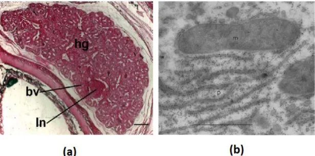
Figure 8. Comparative images acquired from optical microscopy (a) and electron microscopy (b).

Image (a) is a light micrograph of Harderian gland from a neonate Alligator mississipiensis stained with Methyl Green-Pyronin Y (bv-blood vessel; hg-Harderian gland and ln-lymphatic node). Adapted from (Rehorek and Smith 2007). Image (b) is a micrograph of a section of mouse liver stained in a saturated solution of uranyl acetate (m-mitochondria and p-highly dense RNA particles). Adapted from (Watson 1958).

Recent alternatives to the microscopic current approaches have been developed. In order to counter the extensive time dispensed in learning and accustoming to the microscope usage and considering the decrease in use of these devices in medical schools (Randell, Ruddle et al. 2013), these institutions have been using virtual slides (Histopathology slides scanned and stored as digital images), for teaching purposes. These slides allow a greater interaction between the students and the relevant morphological features present in the visualized tissue (Kumar, Velan et al. 2004).

In Leeds University, Randell R. and collaborators have developed a virtual reality microscope that consists of a wall-sized high-definition display (Powerwall) capable of rendering gigapixel virtual slides in real time (Figure 9). This system provides a five times greater slide area than conventional microscopes with equivalent magnification, and since it has a wall-size is better suited for group interpretation. This novel approach enables students to cooperatively interpret the displayed images, showing a more interactive apprenticeship. A complementary study, performed by Treanor D. and co-workers, aimed to verify this new solution for virtual slides analysis as a viable replacement for conventional microscopy in the histopathologists’ investigation and diagnostic routine. In fact, the diagnostic made by consulting virtual slices takes 60% longer, mainly due to the considerable amount of time spent to navigate across the entire image in the small display size, provided by common computer monitors and inadequate user interfaces. With this in mind, the aim of this study was to assess if by increasing the display size, using the Powerwall, the diagnostic would reach similar speed when comparing to conventional microscopy. The performed test in this study involved a simple diagnosis, finding small objects in the image, a decision about a lymph node and score a tissue microarray. By using the virtual microscope, histopathologists performed clinical diagnostics and all the other assigned tasks in similar times as when using a conventional microscope (Treanor, Jordan‐Owers et al. 2009, Randell, Hutchins et al. 2012, Randell, Ruddle et al. 2013).

Figure 9. Leeds University wall-sized virtual

microscope. Adapted from (Randell, Hutchins et al. 2012).

In the University of South Carolina School of Medicine, according to (Blake, Lavoie et al. 2003), the transition and implementation of virtual slides and virtual microscopes for teaching

purposes was performed. The histological slides were scanned and viewed up to a 400x magnification recurring to the MrSID viewer (wavelet-based multiresolution seamless image database, property of LizardTech (Hovanes, Deal et al. 1999)) and the computer as a virtual microscope. The stated approach possesses useful features, including effective microscope and telescope functions providing greater versatility for tissue sample study and increased speed in localizing the structures of interest, when compared to the conventional microscope.

In light of the stated, digital pathology promises interesting advantages, both in terms of efficiency and safety considering conventional microscopy procedures (Randell, Ruddle et al. 2012). Potential advantages associated to a digital system reside in the possibility to alert histopathologists about the presence of new slides or cases to be analyzed (similar to the workflow in radiology diagnostics) and provide an easier cooperation between technicians when investigating a particular case. The latter is extremely important in the workflow of specialists, since this digital method allows a faster and safer way to share microscopic visualizations of tissue samples with other specialists, from other labs and also countries, to obtain second opinions, an extremely important procedure to ensure a flawless diagnostic. With the digital procedure, slides can be simultaneously sent to several histopathologists and, since the physical transportation of those slides is inexistent, there is a reduced risk of losing or mixing them, thus avoiding an erroneous diagnostic (Della Mea, Demichelis et al. 2006, Gilbertson, Ho et al. 2006, Nakhleh 2008). Also with the purpose of providing a fast and accurate second opinion to doctors and histopathologists, several computational methods are being developed to process and analyze digital tissue images. Some of those methods are introduced in following sections.

2.2. Image Processing

The first approach in order to acquire visual features and information from images, in the particular case of this study, from histological images, involves some computational strategies constituting the image processing procedure.

The beginnings of image processing trace back to the middle of the 20th _{century, when it}

started to be applied to improve microscope image’s quality, basically through frequency filtering (signal-to-noise ratio, contrast and image restoration methods). Real developments were made since then, and the analog image processing was replaced by digital image processing with the advent of powerful computers capable of applying sophisticated algorithms to large images in an acceptable amount of time (Bonnet 2004).

Since the visual interpretation is the core of most medical diagnostic procedures and the final diagnostic decision, for cancer and other diseases, is based on tissue examination, medicine represents a large application field for image processing and analysis algorithms (Bengtsson 2003). However, visual interpretation and evaluation present several weaknesses. For pathologists, it is a time-consuming, cumbersome and tedious process to analyze a large number of tissue samples in practice, thus requiring a long time and intensive manual labor to produce viable results. Besides from this problem, visual evaluations can, in many cases, be subject to unacceptable inter and intra-reviewer discrepancies (20% discrepancy between central and institutional reviewers, as reported by Teot L.A. et al. in (Teot, Sposto et al. 2007)), due to the sampling bias, confirming that it represents an error-prone method (Bengtsson 2003, Kong, Sertel et al. 2009, Sertel, Kong et al. 2009).

To overcome the stated weaknesses, established in the currently used visual evaluation process, allied to the fact that digital images are growing in popularity, computational methods resorting to automated image processing and analysis algorithms are being developed (Bengtsson 2003, Kong, Sertel et al. 2009). The automatic processing and analysis of tissue images provides reliable data, accelerates data acquisition process and by allowing digital image management it can replace other evaluation methods, more expensive and impossible to execute (Cisneros, Cordero et al. 2011).

Automated systems can exclude human factor mistakes and increase the speed of diagnostic processes. These systems represent an important asset considering that the amount of experienced specialists that conduct a correct histological analysis is reduced or concentrated in big medical centers. Therefore, this leads to an accumulation of cases poorly or misdiagnosed, conducting to incorrect untimely treatments and ultimately resulting in disablement or death. Considering the abovementioned it is clear the need for automated processes concerning morphology diagnostics in medicine, to improve the diagnostic accuracy and compensate the scarce number of specialists (Nedzved, Belotserkovsky et al. 2005).

The key challenges in histological image computational analysis are automated cellular segmentation and classification in tissue images. Nevertheless, due to the complex nature and variety of histological images, it is difficult to develop automatic segmentation methods applicable to any type of those images (Nedzved, Belotserkovsky et al. 2005, Chomphuwiset, Magee et al. 2011).

The general procedure for automatic image processing and analysis can be divided in several steps, starting with the acquisition of digital histology images, which can range from diverse resolutions depending on the application and the size of the biological structure in study, on the histological sample. The following step is the image processing to identify the target tissues or biological structures in question, comprising, as a standard framework, image enhancement, image segmentation, feature extraction and implementation of machine learning algorithms (Caicedo 2009). To perform each of the previously referred stages a wide variety of computational methods can be implemented, according to different purposes (for example, automation of mass screening of histological specimens or quantitative analysis of a significant structure in the tissue) (Bengtsson 2003).

The image processing and analysis pipeline that is going to be produced in this work consists of three particular steps, the image pre-processing, image segmentation and 3D reconstruction (in section 2.3). A state of the art on methods for both these steps is presented in more detail in further sections.

2.2.1. Image Pre-Processing

Although segmentation is the most important step in image processing and analysis, it is unusual to achieve a consistent and useful segmentation using only a single procedure. In order to obtain a successful segmentation, algorithms typically apply a constructed combination of methods, including a wide variety of preprocessing steps (Beare and Lehmann 2006).

To process histological images, an initial preprocessing step must be applied to reduce the computational costs through multi-scale image decomposition (Gonzalez and Woods 2008). This initial process produces low resolution images that can be analyzed to locate interesting structures and allow the implementation of other image processing steps only on those structures’ pixels. The preprocessing step is meant also to restore the images, by reducing image noise, low intensity contrast and intensity inhomogeneities present in the histological data. To perform this, methods such as image smoothing, denoise and enhancement can be applied (He, Long et al. 2010). Image smoothing is commonly performed recurring to spatial filtering methods used to remove image high frequency noise. Image denoising methods are implemented to remove image noise produced in image acquisition and compression processes (Aubert and Kornprobst 2006) and image enhancement techniques favour an increase in contrast between the regions of interest and the background, being the adaptive filters the most commonly employed methods (Gonzalez and Woods 2008).

Considering the amount of manual labor involved in tissue samples preparation (section 2.1.2), this process tends to introduce certain types of artifacts that require proper image preprocessing techniques to be countered. The majority of artifacts found in histological images are based on orientation differences found in the sections mounted in glass slides, variable luminance gradient (depending on the slide region where the tissue observed), non-tissue noise produced by dust or bubbles and staining variations (variable non-tissue thickness and stain concentrations originate color variations in the histological stained structures). Therefore, image pre-processing techniques are applied to deal with acquisition artifacts and defective histology sections (Mosaliganti, Pan et al. 2006).

Some techniques are specially designed to deal with histological artifacts present in the digital images, namely the defective section exclusion and principal component analysis (PCA) alignment.

In order to improve the 3D reconstruction robustness defective sections have to be identified and removed from the registration process. Since all images are acquired with the same magnification, tissue sizes in consecutive images should not suffer significant variations. Thus, when a large variation is verified it is probably due to broken or defective sections. To eliminate them the relevant structure areas were computed for each image and plotted against section location, using binary masks (masks containing information about the tissue pixel location. Tissue pixels identified and stored as binary masks). Spikes in this plot are potential defective sections (Mosaliganti, Pan et al. 2006).

Principal component analysis alignment is used to estimate tissue orientation, according

to prior knowledge of typical structure arrangement, concerning the studied tissue. Since tissue orientations are used to initialize registration methods (section 2.3), by using this technique, the likelihood of converging to a more reliable global solution is increased (Mosaliganti, Pan et al. 2006).

The staining conditions verified in different histological slices suffer considerable variations (Figure 10). Therefore, after the being digitized, images present considerable color ranges. To normalize color distributions present across the slices, histogram equalization represents a viable solution (Sertel, Catalyurek et al. 2009). Histogram equalization is a well-known and widely used image enhancement technique, due to its simplicity, high performance in almost all types of images. This technique is performed by remapping of grey-levels in an image based on a probability distribution of the input grey-levels, stretching the dynamic range of the image histogram. Thus, resulting in overall image contrast enhancement. The drawbacks of this method are noticeable in images with high and low mean brightness. The result is a significant change in the image outlook, whereas the purpose was only to enhance the contrast. Histogram equalization is best suited to enhance the edges between different structures, but, in return, reduces local details within those structures, producing over enhancement and saturation artefacts (Kaur, Kaur et al. 2011). The histogram equalization procedure is based on the assumption that the processed image presents uniform image quality in all regions, and therefore, one single grayscale mapping provides similar contrast enhancement throughout all

these regions. But, when distributions of grayscale intensities are variable according to different regions in the image, the previous assumption is invalid. Facing this, an adaptive histogram equalization technique, capable of determining the mapping for each pixel based on its local grayscale distribution (surrounding pixels), could significantly outperform the standard method. However, when grayscale distribution is highly localized, full histogram equalization might not be desirable to transform very low contrast images. By limiting the contrast allowed through histogram equalization, the possibility of two very close grayscales being mapped to significantly different grayscales, i.e. high slope segments present in the grayscale mapping curve, can be avoided. Combining the contrast limiting approach with the previously mentioned adaptive histogram equalization method, the result is referred to as Contrast Limited Adaptive

Histogram Equalization (CLAHE) (Reza 2004).

Figure 10. Sequence of histological images from MKI (Mitosis-karyorrhexis index) cells, varying in color

information due to staining differences. Adapted from (Sertel, Catalyurek et al. 2009).

For medical images, color enhancement represents a valuable tool to aid in visualization, detection and segmentation of specific tissue structures. An effective approach to increase color contrast on an image and maintain its hue (the pure color) is to transform the RGB (R - Red, G - Green, B - Blue) color into HSV (Hue, Saturation, Value) color space, modifying only the saturation (luminance) value in the image’s pixels. The transformation is given by:

𝐻 = 𝑐𝑜𝑠

× (

)

𝑆 = 1 −

[min⁡(𝑅, 𝐺, 𝐵)]

(

𝑉 =

(𝑅 + 𝐺 + 𝐵)

The luminance manipulation, through grey-level enhancement processes, without affecting the other two components in HSV color is possible due to the lack of correlation between these components. The usual process starts by performing the color transform to

convert the image in HSV color where the luminance or color saturation can be modified, disregarding the other components. Then, the reverse transform back to RGB color is applied in order to ascertain the effects of the produced modification (Bautista and Yagi 2010).

Hukkanen J. and co-.workers implemented a pre-processing method to improve the efficiency of nuclei segmentation (more information in section 2.2.2.) in histological images. The pre-processing method performs the conversion of H & E stained histological images originally in RGB color space into CIE L*a*b color space. The L component, the luminosity component, is then denoted as a grey-level image, which is further processed to obtain the segmentation. The L*a*b color space consists of a luminosity layer “L*”, a chromaticity layer “a*” (indicating the color location in the red-green axis) and a chromaticity layer “b*” (indicating the color location in the blue-yellow axis)(Hukkanen, Hategan et al. 2010).

In (Tabesh, Teverovskiy et al. 2007) is presented a study concerning image features for cancer diagnosis and histological grading of prostate images. The features representing color, texture and morphological details were combined in a supervised learning framework. The first stage in this framework involved pre-processing techniques, including background removal and image histogram matching to a reference image. The background was identified and then removed from the analysis through color tissue image transformation, from RGB color space into YCbCr color space (Gonzalez and Woods 2008), and posterior thresholding (section 2.2.2.) of the luminance (Y) component with a global empirically determined threshold. After this, the binary mask containing the tissues of interest is refined via closing and opening operations to fill gaps between tissue structures and remove small artefacts from the image. A convex hull operation (Gonzalez and Woods 2008) is then, applied to ensure the integration of lumens as tissue of interest, avoiding its exclusion from the binary mask. The second pre-processing step, implemented in this study, consisted of an histogram matching between the analysed histological image and a reference image, through the transformation⁡𝐹𝑟−1[𝐹𝑖(𝑥)], where 𝑥 is

the pixel value in each of the red, blue and green channels. 𝐹𝑟 and 𝐹𝑖 are, the cumulative

distribution function of pixel values for the input and reference images, respectively. Histogram matching is performed to mitigate color variations produced by staining and illumination conditions, which can affect segmentation efficiency.

The Stain Deconvolution technique is a pre-processing method, based on color deconvolution, which aims to deconvolve the applied stains on a certain RGB color image, to generate separate images, where each grayscale image shows the distribution of a single stain. This algorithm assumes that the chemical stains implemented to dye the tissue slides follows the Beer-Lambert Law of absorption, which provides a logarithmic relationship between the original RGB color channels and a stain matrix. This complex methodology is presented by both

(Ruifrok and Johnston 2001, Unpublished 2015), and the algorithm behind it is further explained in this work, on section 3.2.3.

2.2.2. Image Segmentation

After image enhancement produced by pre-processing methods, removing the noise and increasing the contrast between the structures of interest and the remainder tissue, a new step, called segmentation, can be performed.

Segmentation is the most important part in image processing and analysis, and consists of a grouping process, in which the group components share similarities concerning one or more features, ultimately identifying regions in the input image corresponding to distinct structures (Vernon 1991).

The segmentation is the first step to perform automatic analysis of histology images, apart from the image pre-processing, enabling the distinction of some particular biological tissue from the remainder components in the image. Staining techniques are performed in histology to facilitate human visual identification of the different components, for a specialist, but in order to implement other computational processes on those components the segmentation must be performed (Cisneros, Cordero et al. 2011). The application of this step is suited for a multitude of purposes, such as effective identification of tissues, image subdivision for portionwise processing or pattern modelling (Caicedo 2009).

Since a universal segmentation, valid and suitable for all the image applications, does not exist, a specialized method is required for each application(Cisneros, Cordero et al. 2011). There are two different approaches to perform image segmentation: Region based and boundary based methods (Vernon 1991).

Region based methods focus on reconstructing the various components of an image into

two dimensional areas (regions), by implementing a similarity criterion from the pixels of each elemental area (Cisneros, Cordero et al. 2011). An example of these segmentation methods are Region-Growing techniques, that, starting from one or more points (seeds), initialized manually or automatically by heuristic methods, they are expanded to neighbour pixels that share a certain homogeneity criterion (Pham, Xu et al. 2000).

Boundary based segmentation concerns on the detection of boundary pixels of the

structures present in the image, extracting them from the rest. The isolated boundary is then used not only to define the location but also the shape of the structure of interest. Boundary detection algorithms diverge on the amount of domain-dependent information incorporated when the connection of edges is performed. Therefore, the effectiveness of these methods is intimately dependent on the performance of edge detection algorithms (Vernon 1991). Segmentation performed with edge detection techniques implements minimum cost functions and certain filters, based on the gradient concept, to determine the borders of homogeneous sections of the image. Considering that usually these detectors do not provide closed elements,