arXiv:1602.01633v2 [hep-ex] 17 Nov 2016
EUROPEAN ORGANISATION FOR NUCLEAR RESEARCH (CERN)
Phys. Lett. B758 (2016) 67
DOI:10.1016/j.physletb.2016.04.050
CERN-EP-2016-014 18th November 2016
Charged-particle distributions in
√ s = 13 TeV pp interactions
measured with the ATLAS detector at the LHC
The ATLAS Collaboration
Abstract
Charged-particle distributions are measured in proton–proton collisions at a centre-of-mass energy of 13 TeV, using a data sample of nearly 9 million events, corresponding to an in-tegrated luminosity of 170 µb−1, recorded by the ATLAS detector during a special Large Hadron Collider fill. The charged-particle multiplicity, its dependence on transverse mo-mentum and pseudorapidity and the dependence of the mean transverse momo-mentum on the charged-particle multiplicity are presented. The measurements are performed with charged particles with transverse momentum greater than 500 MeV and absolute pseudorapidity less than 2.5, in events with at least one charged particle satisfying these kinematic requirements. Additional measurements in a reduced phase space with absolute pseudorapidity less than 0.8 are also presented, in order to compare with other experiments. The results are cor-rected for detector effects, presented as particle-level distributions and are compared to the predictions of various Monte Carlo event generators.
c
2016 CERN for the benefit of the ATLAS Collaboration.
1. Introduction
Charged-particle measurements in proton–proton (pp) collisions provide insight into the strong interac-tion in the low-energy, non-perturbative region of quantum chromodynamics (QCD). Particle interacinterac-tions at these energy scales are typically described by QCD-inspired models implemented in Monte Carlo (MC) event generators with free parameters that can be constrained by such measurements. An accurate description of low-energy strong interaction processes is essential for simulating single pp interactions as well as the effects of multiple pp interactions at high instantaneous luminosity in hadron colliders. Charged-particle distributions have been measured previously in pp and proton–antiproton collisions at various centre-of-mass energies [1–7] (and references therein).
This paper presents inclusive measurements of primary charged-particle distributions in pp collisions at a centre-of-mass energy of √s = 13 TeV, using data recorded by the ATLAS experiment [8] at the Large Hadron Collider (LHC) corresponding to an integrated luminosity of approximately 170 µb−1. Here in-clusive means that all processes in pp interactions are included and no attempt to correct for certain types of process, such as diffraction, is made. These measurements, together with previous results, shed light on the evolution of charged-particle multiplicities with centre-of-mass energy, which is poorly constrained. A strategy similar to that in Ref. [1] is used, where more details of the analysis techniques are given. The distributions are measured using tracks from primary charged particles, corrected for detector effects, and are presented as inclusive distributions in a well-defined kinematic region. Primary charged particles are defined as charged particles with a mean lifetime τ > 300 ps, either directly produced in pp interactions or from subsequent decays of directly produced particles with τ < 30 ps; particles produced from decays of particles with τ > 30 ps, called secondary particles, are excluded. This definition differs from earlier analyses in that charged particles with a mean lifetime 30 < τ < 300 ps were previously included. These are charged strange baryons and have been removed due to the low efficiency of reconstructing them.1 All primary charged particles are required to have a momentum component transverse to the beam direction,2
pT, of at least 500 MeV and absolute pseudorapidity, |η|, less than 2.5. Each event is required to have at least one primary charged particle.
In these events the following distributions are measured: 1 Nev · dNch dη , 1 Nev · 1 2πpT · d2Nch dηdpT , and 1 Nev · dNev dnch
as well as the mean pT (hpTi) of all primary charged particles versus nch. Here nch is the number of primary charged particles in an event, Nev is the number of events with nch ≥ 1, and Nch is the total number of primary charged particles in the data sample.3 The measurements are also presented in a phase space that is common to the ATLAS, CMS [9] and ALICE [10] detectors in order to ease comparison between experiments. For this purpose an additional requirement of |η| < 0.8 is made for all primary charged particles. These results are presented in Appendix A. Finally, the mean number of primary
1Since strange baryons tend to decay within the detector volume, especially if they have low momentum, they often do not
leave enough hits to reconstruct a track, leading to a track reconstruction efficiency of approximately 0.3%.
2ATLAS uses a right-handed coordinate system with its origin at the nominal interaction point (IP) in the centre of the detector
and the z-axis along the beam pipe. The x-axis points from the IP to the centre of the LHC ring, and the y-axis points upward. Cylindrical coordinates (r, φ) are used in the transverse plane, φ being the azimuthal angle around the beam pipe. The pseudorapidity is defined in terms of the polar angle θ as η = − ln tan(θ/2).
3The factor 2πp
T in the pTspectrum comes from the Lorentz-invariant definition of the cross section in terms of d3p. The
charged particles for η = 0 is compared to previous measurements at different centre-of-mass energies. The measurements are compared to particle-level MC predictions.
The remainder of this paper is laid out as follows. The relevant components of the ATLAS detector are described in Section2. The MC event generators and detector simulation used in the analysis are in-troduced in Section3. The selection criteria applied to the data and the contributions from background events are discussed in Sections4and5respectively. The selection efficiency and corresponding correc-tions to the data are discussed in Seccorrec-tions6 and 7respectively. The corrected results are compared to theoretical predictions in Section8and a conclusion is given in Section9. The measurement of primary charged particles in the reduced phase space of |η| < 0.8 is presented in AppendixA.
2. ATLAS detector
The ATLAS detector covers almost the whole solid angle around the collision point with layers of tracking detectors, calorimeters and muon chambers. For the measurements presented in this paper, the tracking devices and the trigger system are of particular importance.
The inner detector (ID) has full coverage in φ and covers the pseudorapidity range |η| < 2.5. It consists of a silicon pixel detector (pixel), a silicon microstrip detector (SCT) and a transition radiation straw-tube tracker (TRT). These detectors span a sensitive radial distance from the interaction point of 33–150 mm, 299–560 mm and 563–1066 mm respectively, and are situated inside a solenoid that provides a 2 T axial magnetic field. The barrel (each end-cap) consists of four (three) pixel layers, four (nine) double-layers of single-sided silicon microstrips with a 40 mrad stereo angle between the inner and outer part of a double-layer, and 73 (160) layers of TRT straws. The innermost pixel double-layer, the insertable B-layer (IBL) [11], was added between Run 1 and Run 2 of the LHC, around a new narrower (radius of 25 mm) and thinner beam pipe. It is composed of 14 lightweight staves arranged in a cylindrical geometry, each made of 12 silicon planar sensors in its central region and 2 × 4 3D sensors at the ends. The IBL pixel dimensions are 50 × 250 µm2in the φ and z directions (compared with 50 × 400 µm2for other pixel layers). The smaller radius and the reduced pixel size result in improvements of both the transverse and longitudinal impact parameter resolutions. In addition, new services have been implemented which significantly reduce the material at the boundaries of the active tracking volume. A track from a charged particle traversing the barrel detector typically has 12 silicon measurement points (hits), of which four are pixel and eight SCT, and more than 30 TRT straw hits.
The ATLAS detector employs a two-level trigger system: the level-1 hardware stage (L1) and the high-level trigger software stage (HLT). This measurement uses the L1 decision from the minimum-bias trigger scintillators (MBTS), which were replaced between Run 1 and Run 2. The MBTS are mounted at each end of the detector in front of the liquid-argon end-cap calorimeter cryostats at z = ±3.56 m and segmented into two rings in pseudorapidity (2.07 < |η| < 2.76 and 2.76 < |η| < 3.86). The inner ring is segmented into eight azimuthal sectors while the outer ring is segmented into four azimuthal sectors, giving a total of twelve sectors per side. The MBTS trigger selection used for this paper requires one counter above threshold from either side of the detector and is referred to as a single-arm trigger. The efficiency of this trigger is studied with an independent control trigger. The control trigger selects events randomly at L1 which are then filtered at HLT by requiring at least one reconstructed track with pT>200 MeV.
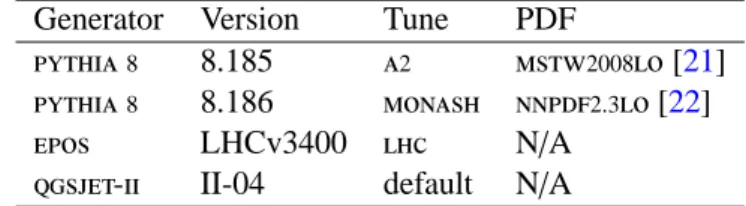
Table 1: Summary of MC tunes used to compare to the corrected data. The generator and its version are given in the first two columns, the tune name and the PDF used are given in the next two columns.
Generator Version Tune PDF
pythia8 8.185 a2 mstw2008lo[21] pythia8 8.186 monash nnpdf2.3lo[22]
epos LHCv3400 lhc N/A
qgsjet-ii II-04 default N/A
3. Monte Carlo event generator simulation
The pythia8 [12], epos [13] and qgsjet-ii [14] MC generators are used to correct the data for detector effects and to compare with particle-level corrected data. A brief introduction to the relevant parts of these event generators is given below.
In pythia8 inclusive hadron–hadron interactions are described by a model that splits the total inelastic cross section into non-diffractive (ND) processes, dominated by t-channel gluon exchange, and diffractive processes involving a colour-singlet exchange. The simulation of ND processes includes multiple parton– parton interactions (MPI). The diffractive processes are further divided into single-diffractive dissociation (SD), where one of the initial protons remains intact and the other is diffractively excited and dissociates, and double-diffractive dissociation (DD) where both protons dissociate. The sample contains approx-imately 22% SD and 12% DD processes. Such events tend to have large gaps in particle production at central rapidity. A pomeron-based approach is used to describe these events [15].
eposprovides an implementation of a parton-based Gribov–Regge [16] theory, which is an effective QCD-inspired field theory describing hard and soft scattering simultaneously.
qgsjet-ii provides a phenomenological treatment of hadronic and nuclear interactions in the Reggeon field theory framework [17]. The soft and semi-hard parton processes are included in the model within the “semi-hard pomeron” approach. epos and qgsjet-ii calculations do not rely on the standard parton distribution functions (PDFs) as used in generators such as pythia8.
Different settings of model parameters optimised to reproduce existing experimental data are used in the simulation. These settings are referred to as tunes. For pythia8 two tunes are used, a2[18] and mon-ash[19]; for epos the lhc [20] tune is used. qgsjet-ii uses the default tune from the generator. Each tune utilises 7 TeV minimum-bias data and is summarised in Table1, together with the version of each gener-ator used to produce the samples. The pythia8a2sample, combined with a single-particle MC simulation used to populate the high-pT region, is used to derive the detector corrections for these measurements. All the events are processed through the ATLAS detector simulation program [23], which is based on geant4[24]. They are then reconstructed and analysed by the same program chain used for the data.
4. Data selection
The data were recorded during a period with a special configuration of the LHC with low beam currents and reduced beam focusing, and thus giving a low expected mean number of interactions per bunch
crossing, hµi = 0.005. Events were selected from colliding proton bunches using a trigger which required one or more MBTS counters above threshold on either side of the detector.
Each event is required to contain a primary vertex, reconstructed from at least two tracks with a min-imum pT of 100 MeV, as described in Ref. [25]. To reduce contamination from events with more than one interaction in a bunch crossing, events with a second vertex containing four or more tracks are re-moved. Events where the second vertex has fewer than four tracks are not rere-moved. These are dominated by contributions where a secondary interaction is reconstructed as another primary vertex or where the primary vertex is split into two vertices, one with few tracks. The fraction of events rejected by the veto on additional vertices due to split vertices or secondary interactions is estimated in the simulation to be 0.02%, which is negligible and therefore ignored.
Track candidates are reconstructed [26,27] in the silicon detectors and then extrapolated to include meas-urements in the TRT. Events are required to contain at least one selected track, passing the following criteria: pT > 500 MeV and |η| < 2.5; at least one pixel hit and at least six SCT hits, with the additional requirement of an innermost-pixel-layer hit if expected4 (if a hit in the innermost layer is not expected, the next-to-innermost hit is required if expected); |dBL
0 | < 1.5 mm, where the transverse impact parameter,
dBL0 , is calculated with respect to the measured beam line position; and |zBL0 · sin θ| < 1.5 mm, where zBL0 is the difference between the longitudinal position of the track along the beam line at the point where d0BLis measured and the longitudinal position of the primary vertex, and θ is the polar angle of the track. Finally, in order to remove tracks with mismeasured pTdue to interactions with the material or other effects, the track-fit χ2probability is required to be greater than 0.01 for tracks with pT > 10 GeV. There are 8.87 million events selected, containing a total of 106 million selected tracks.
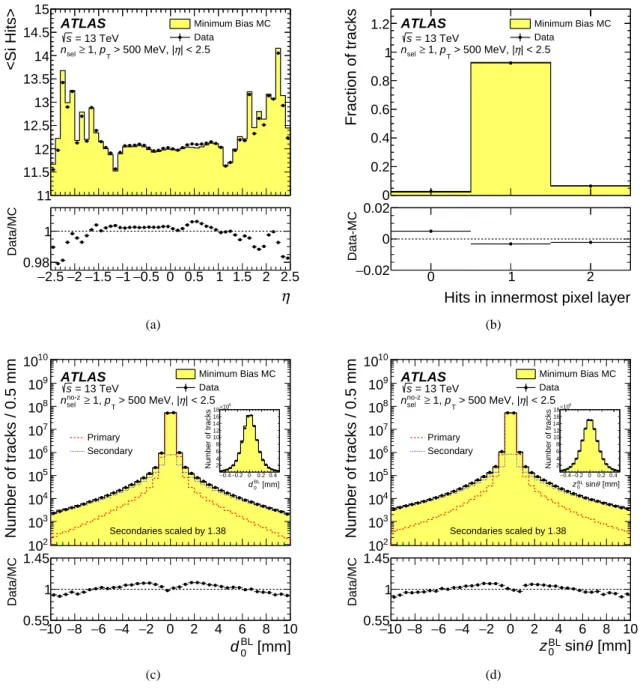
The performance of the ID track reconstruction in the 13 TeV data and its simulation is studied in Ref. [28]. Overall, good agreement between data and simulation is observed. Figure 1 shows selected performance plots particularly relevant to this analysis. Figure1(a)shows the average number of silicon hits as a function of η. There is reasonably good agreement, although discrepancies of up to 2% (in the end-caps) are seen; however, these have a small effect on the track reconstruction efficiency. The discrepancies are due to differences between data and simulation in the number of operational detector elements and an imperfect description of the amount of detector material between the pixel detector and the SCT. The impact on the results of these discrepancies is discussed in Section6.3. Figure1(b)shows the fraction of tracks with a given number of IBL hits per track. There is a difference of 0.5% between data and simulation in the fraction of tracks with zero IBL hits, coming predominantly from a difference in the rate of tracks from secondary particles, which is discussed in more detail in Section5. A systematic uncertainty due to the small remaining difference in the efficiency of the requirement of at least one IBL hit is discussed in Section6. Figures1(c)and1(d)show the dBL0 and zBL0 · sin θ distributions respectively. In these figures the fraction of tracks from secondary particles in simulation is scaled to match the frac-tion seen in data, and the separate contribufrac-tions from tracks from primary and secondary particles are shown. This, along with the differences between simulation and data, which have a negligible impact on the analysis, are discussed in Section5.
η <Si Hits> 11 11.5 12 12.5 13 13.5 14 14.5 15 Minimum Bias MC Data ATLAS | < 2.5 η > 500 MeV, | T p 1, ≥ sel n = 13 TeV s η 2.5 − −2−1.5−1−0.5 0 0.5 1 1.5 2 2.5 Data/MC 0.98 1 (a)
Hits in innermost pixel layer
Fraction of tracks 0 0.2 0.4 0.6 0.8 1 1.2 Minimum Bias MC Data ATLAS | < 2.5 η > 500 MeV, | T p 1, ≥ sel n = 13 TeV s
Hits in innermost pixel layer
0 1 2 Data-MC 0.02 − 0 0.02 (b) [mm] BL 0 d Number of tracks / 0.5 mm 2 10 3 10 4 10 5 10 6 10 7 10 8 10 9 10 10 10 Minimum Bias MC Data Primary Secondary | < 2.5 η > 500 MeV, | T p 1, ≥ no-z sel n = 13 TeV s ATLAS Secondaries scaled by 1.38 [mm] BL 0 d 10 − −8 −6 −4 −2 0 2 4 6 8 10 Data/MC 0.55 1 1.45 [mm] BL 0 d 0.4 − −0.20 0.2 0.4 Number of tracks 2 4 6 8 10 12 14 16 18 6 10 × (c) [mm] θ sin BL 0 z Number of tracks / 0.5 mm 2 10 3 10 4 10 5 10 6 10 7 10 8 10 9 10 10 10 Minimum Bias MC Data Primary Secondary | < 2.5 η > 500 MeV, | T p 1, ≥ no-z sel n = 13 TeV s ATLAS Secondaries scaled by 1.38 [mm] θ sin BL 0 z 10 − −8 −6 −4 −2 0 2 4 6 8 10 Data/MC 0.55 1 1.45 [mm] θ sin BL 0 z 0.4 − −0.20 0.2 0.4 Number of tracks 2 4 6 8 10 12 14 16 18 6 10 × (d)
Figure 1: Comparison between data and pythia8a2simulation for (a) the average number of silicon hits per track, before the requirement on the number of SCT hits is applied, as a function of pseudorapidity, η; (b) the number of innermost-pixel-layer hits on a track before the requirement on the number of innermost-pixel-layer hits is applied; (c) the transverse impact parameter distribution of the tracks, prior to any requirement on the transverse impact parameter, calculated with respect to the average beam position, dBL
0 ; and (d) the difference between the longitudinal
position of the track along the beam line at the point where dBL
0 is measured and the longitudinal position of the
primary vertex projected to the plane transverse to the track direction, zBL
0 · sin θ, prior to any requirement on
zBL
0 · sin θ. The uncertainties are the statistical uncertainties of the data. In (c) and (d) the separate contributions
from tracks coming from primary and secondary particles are also shown and the fraction of secondary particles in the simulation is scaled by 1.38 to match that seen in the data, with the final simulation distributions normalised to the number of tracks in the data. The inserts in the panels for (c) and (d) show the distributions on a linear scale.
5. Background contributions and non-primary tracks
The contribution from non-collision background events, such as proton interactions with residual gas molecules in the beam pipe, is estimated using events that pass the full event selection but occur when only one of the two beams is present. After normalising to the contribution expected in the selected data sample (using the difference in the time of the MBTS hits on each side of the detector, which is possible as background events with hits on only one side are negligible) a contribution of less than 0.01% of events is found from this source, which is negligible and therefore neglected. Background events from cosmic rays, estimated by considering the expected rate of cosmic-ray events compared to the event readout rate, are also found to be negligible and therefore neglected.
The majority of events with more than one interaction in the same bunch crossing are removed by the rejection of events with more than one primary vertex. Some events may survive because the interactions are very close in z and are merged together. The probability to merge vertices is estimated by inspecting the distribution of the difference in the z position of pairs of vertices (∆z). This distribution displays a de-ficit around ∆z = 0 due to vertex merging. The magnitude of this effect is used to estimate the probability of merging vertices, which is 3.2%. When this is combined with the number of expected additional inter-actions for hµi = 0.005, the remaining contribution from tracks from additional interinter-actions is found to be less than 0.01%, which is negligible and therefore neglected. The additional tracks in events in which the second vertex has fewer than four associated tracks are mostly rejected by the zBL0 · sin θ requirement, and the remaining contribution is also negligible and neglected.
The contribution from tracks originating from secondary particles is subtracted from the number of re-constructed tracks before correcting for other detector effects. These particles are due to hadronic in-teractions, photon conversions and decays of long-lived particles. There is also a contribution of less than 0.1% from fake tracks (those formed by a random combination of hits or from a combination of hits from several particles); these are neglected. The contribution of tracks from secondary particles is estimated using simulation predictions for the shapes of the dBL0 distributions for tracks from primary and secondary particles satisfying all track selection criteria except the one on dBL0 . These predictions form templates that are fit to the data in order to extract the relative contribution of tracks from secondary particles. The Gaussian core of the distribution is dominated by the tracks from primary particles, with a width determined by their d0BL resolution; tracks from secondary particles dominate the tails. The fit is performed in the region 4 < |dBL0 | < 9.5 mm, in order to reduce the dependence on the description of the dBL0 resolution, which affects the core of the distribution. From the fit, it was determined that the fraction of tracks from secondary particles in simulation needs to be scaled by a factor 1.38 ± 0.14. This indicates that (2.3 ± 0.6) % of tracks satisfying the final track selection criteria (|dBL0 | < 1.5 mm) originate from secondary particles, where systematic uncertainties are dominant and are discussed below. Of these tracks 6% come from photon conversions and the rest from hadronic interactions or long-lived decays. The description of the η and pT dependence of this contribution is modelled sufficiently accurately by the simulation that no additional correction is required. Figure1(c)shows the dBL0 distribution for data compared to the simulation with the fraction of tracks from secondary particles scaled to the fitted value. A small disagreement is observed in the core of the dBL0 distribution. This has no impact in the tail of the distribution used for the fit. The dominant systematic uncertainty stems from the interpolation of the number of tracks from secondary particles from the fit region to the region |dBL0 | < 1.5 mm. Different generators are used to estimate the interpolation and differences between data and simulation in the shape of the dBL0 distribution in the fit region are considered. Additional, much smaller, systematic uncertainties
arise from a variation of the fit range, considering the η dependence of the fitted fractions and from using special simulation samples with varying amounts of detector material.
There is a second source of non-primary particles: charged particles with a mean lifetime 30 < τ < 300 ps which, unlike in previous analyses [1], are excluded from the primary-particle definition. These are charged strange baryons that decay after a short flight length and have a very low track reconstruction efficiency. Reconstructed tracks from these particles are treated as background and are subtracted. The fraction of reconstructed tracks coming from strange baryons is estimated from simulation with epos to be (0.01 ± 0.01)% on average, with the fraction increasing with track pT to be (3 ± 1)% above 20 GeV. The fraction is much smaller at low pT due to the extremely low efficiency of reconstructing a track from a particle that decays early in the detector. The systematic uncertainty is taken as the maximum difference between the nominal epos prediction and that of pythia8a2or pythia8monash, which is then symmetrised.
6. Selection e
fficiency
The data are corrected to obtain inclusive spectra for primary charged particles satisfying the particle-level kinematic requirements. These corrections account for inefficiencies due to trigger selection, vertex and track reconstruction.
In the following sections the methods used to obtain these efficiencies, as well as the systematic uncer-tainties associated with them, are described.
6.1. Trigger efficiency
The trigger efficiency, εtrig, is measured from a data sample selected using the control trigger described in Section2. The requirement of an event primary vertex is removed for these trigger studies, to account for possible correlations between the trigger and vertex reconstruction efficiencies. The trigger efficiency is therefore parameterised as a function of nno−z
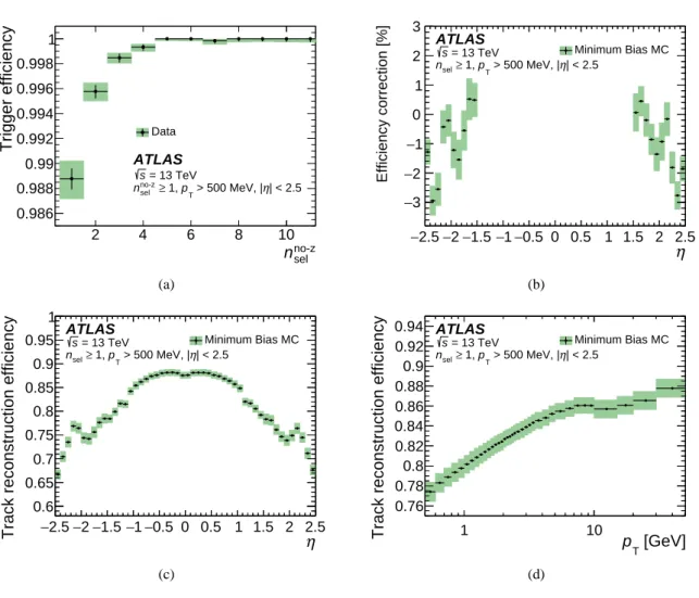
sel , which is defined as the number of tracks passing all of the track selection requirements except for the zBL0 · sin θ constraint, as this requires knowledge of the primary vertex position. The trigger efficiency is taken to be the fraction of events from the control trigger in which the MBTS trigger also accepted the event. This is shown in Figure2(a) as a function of nno−zsel . The efficiency is measured to be just below 99% for nno−zsel = 1 and it rapidly rises to 100% at higher track multiplicities. The trigger requirement is found to introduce no observable bias in the
pT and η distributions of selected tracks. Systematic uncertainties are estimated from differences in the trigger efficiency measured on each of the two sides of the detector and from a study that assesses the impact of beam-induced background and tracks from secondary particles by varying the impact parameter requirements on selected tracks. The total systematic uncertainty is ±0.15% for nno−zsel = 1 and it rapidly decreases at higher track multiplicities. This uncertainty is negligible compared to those from other sources and is therefore neglected.
6.2. Vertex reconstruction efficiency
The vertex reconstruction efficiency, εvtx, is determined from data by taking the ratio of the number of selected events with a reconstructed vertex to the total number of events with the requirement of a
no-z sel n 2 4 6 8 10 Trigger efficiency 0.986 0.988 0.99 0.992 0.994 0.996 0.998 1 Data | < 2.5 η > 500 MeV, | T p 1, ≥ no-z sel n = 13 TeV s ATLAS (a) η 2.5 − −2−1.5−1−0.5 0 0.5 1 1.5 2 2.5 Efficiency correction [%] 3 − 2 − 1 − 0 1 2 3 Minimum Bias MC | < 2.5 η > 500 MeV, | T p 1, ≥ sel n = 13 TeV s ATLAS (b) η 2.5 − −2−1.5−1−0.5 0 0.5 1 1.5 2 2.5
Track reconstruction efficiency
0.6 0.65 0.7 0.75 0.8 0.85 0.9 0.95 1 Minimum Bias MC | < 2.5 η > 500 MeV, | T p 1, ≥ sel n = 13 TeV s ATLAS (c) [GeV] T p 1 10
Track reconstruction efficiency
0.76 0.78 0.8 0.82 0.84 0.86 0.88 0.9 0.92 0.94 Minimum Bias MC | < 2.5 η > 500 MeV, | T p 1, ≥ sel n = 13 TeV s ATLAS (d)
Figure 2: (a) Trigger efficiency with respect to the event selection, as a function of the number of reconstructed tracks without the zBL
0 · sin θ constraint (nno−zsel ). (b) Data-driven correction to the track reconstruction efficiency as a
function of pseudorapidity, η. The track reconstruction efficiency after this correction as a function of (c) η and (d) transverse momentum, pTas predicted by pythia8a2and single-particle simulation. The statistical uncertainties are shown as black vertical bars, the total uncertainties as green shaded areas.
primary vertex removed. The expected contribution from beam background events is estimated using the same method as described in Section5and subtracted before measuring the efficiency. Like the trigger efficiency, the vertex efficiency is measured in bins of nno−zsel as the zBL0 · sin θ constraint cannot be applied to the tracks in this study. The efficiency is measured to be just below 90% for nno−zsel = 1 and it rapidly rises to 100% at higher track multiplicities. In events with nno−zsel = 1 the efficiency is also measured as a function of η of the track, and the efficiency increases monotonically from 81% at |η| = 2.5 to 93% at |η| = 0. The systematic uncertainty is estimated from the difference between the vertex reconstruction efficiency measured prior to and after beam background removal. The uncertainty is ±0.1% for nno−zsel = 1 and rapidly decreases at higher track multiplicities. This uncertainty is negligible compared to those from other sources and is therefore neglected.
6.3. Track reconstruction efficiency
The primary track reconstruction efficiency, εtrk, is determined from the simulation, corrected to account for differences between data and simulation in the amount of detector material between the pixel and SCT detectors in the region |η| > 1.5. In the other regions of the detector there is an uncertainty due to the knowledge of the detector material that will be discussed below, but no correction is applied. The efficiency is parameterised in two-dimensional bins of pTand η and is defined as:
εtrk(pT, η) =
Nrecmatched(pT, η)
Ngen(pT, η)
,
where pT and η are generated particle properties, Nrecmatched(pT, η) is the number of reconstructed tracks matched to a generated primary charged particle and Ngen(pT, η) is the number of generated primary charged particles in that bin. A track is matched to a generated particle if the weighted fraction of hits on the track which originate from that particle exceeds 50%. The hits are weighted such that all subdetectors have the same weight in the sum.
The track reconstruction efficiency depends on the amount of material in the detector, due to particle interactions that lead to efficiency losses. The relatively large amount of material between the pixel and SCT detectors in the region |η| > 1.5 has changed between Run 1 and Run 2 due to the replacement of some pixel services, which are difficult to simulate accurately. The track reconstruction efficiency in this region is corrected using a method that compares the efficiency to extend a track reconstructed in the pixel detector into the SCT in data and simulation. Differences in this extension efficiency are sensitive to dif-ferences in the amount of material in this region. The correction together with the systematic uncertainty, coming predominantly from the uncertainty of the particle composition in the simulation used to make the measurement, is shown in Figure2(b). The uncertainty in the track reconstruction efficiency resulting from this correction is ±0.4% in the region |η| > 1.5.
The resulting reconstruction efficiency as a function of η integrated over pT is shown in Figure 2(c). The track reconstruction efficiency is lower in the region |η| > 1 due to particles passing through more material in that region. The slight increase in efficiency at |η| ∼ 2.2 is due to the particles passing through an increasing number of layers in the ID end-cap. Figure2(d)shows the efficiency as a function of pT integrated over η.
A good description of the material in the detector in the regions not probed by the method described above (which only probes the material between the pixel and SCT detectors in the region |η| > 1.5) is needed to obtain a good description of the track reconstruction efficiency. The material within the ID was studied
extensively during Run 1 [29], where the amount of material was known to within ±5%. This gives rise
to a systematic uncertainty in the track reconstruction efficiency of ±0.6% (±1.2%) in the most central (forward) region. Between Run 1 and Run 2 the IBL was installed, the simulation of which must therefore be studied with the Run 2 data. Two data-driven methods are used: a study of secondary vertices from photon conversions (γ → e+e−) and a study of secondary vertices from hadronic interactions, where the radial position of the vertex is measured with good precision. Comparisons between data and simulation indicate that the material in the IBL is constrained to within ±10%. This leads to an uncertainty in the track reconstruction efficiency of ±0.1% (±0.2%) in the central (forward) region. This uncertainty is added linearly to the uncertainty from constraints from Run 1, to cover the possibility of missing material in the simulation in both cases. The resulting uncertainty is added in quadrature to the uncertainty from the data-driven correction. The total uncertainty due to the imperfect knowledge of the detector material is ±0.7% in the most central region and ±1.5% in the most forward region.
There is a small difference in efficiency, between data and simulation, of the requirement that each recon-structed track has at least one pixel hit, at least six SCT hits, an innermost-pixel-layer hit if expected (if a hit in the innermost layer is not expected, the next-to-innermost hit is required if expected) and a track-fit χ2 probability greater than 0.01 for tracks with pT > 10 GeV. This difference is assigned as a further systematic uncertainty, amounting to ±0.5% for pT<10 GeV and ±0.7% for pT>10 GeV.
The total uncertainty due to the track reconstruction efficiency determination, shown in Figures 2(c)
and 2(d), is obtained by adding all effects in quadrature and is dominated by the uncertainty from the material description.
7. Correction procedure
The following steps are taken to correct the measurements for detector effects.
• All distributions are corrected for the loss of events due to the trigger and vertex requirements by reweighting events according to the function:
wev(nno−zsel , η) = 1 εtrig(nno−zsel ) ·
1 εvtx(nno−zsel , η)
,
where the η dependence is only relevant for nno−zsel = 1, as discussed in Section6.2. • The η and pT distributions of selected tracks are corrected using a track-by-track weight:
wtrk(pT, η) = 1 − fsec
(pT, η) − fsb(pT) − fokr(pT, η) εtrk(pT, η)
where fsec and fsb are the fraction of tracks from secondary particles and from strange baryons respectively, determined as described in Section5. The fraction of selected tracks for which the corresponding primary particle is outside the kinematic range, fokr(pT, η), originates from resolu-tion effects and is estimated from the simularesolu-tion to be 3.5% at pT= 500 MeV, decreasing to 1% for
pT = 1 GeV and is only relevant for 2.4 < |η| < 2.5. No additional corrections are needed for the ηdistribution. For the pT distribution a Bayesian unfolding [30] is applied to correct the measured track pTdistribution to that for primary particles.
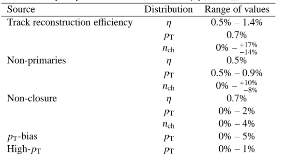
Table 2: Summary of systematic uncertainties on the η, pTand nchdistributions.
Source Distribution Range of values
Track reconstruction efficiency η 0.5% – 1.4%
pT 0.7% nch 0% –+17%−14% Non-primaries η 0.5% pT 0.5% – 0.9% nch 0% –+10%−8% Non-closure η 0.7% pT 0% – 2% nch 0% – 4% pT-bias pT 0% – 5% High-pT pT 0% – 1%
• After applying the trigger and vertex efficiency corrections, the Bayesian unfolding is applied to the multiplicity distribution in order to correct from the observed track multiplicity to the multiplicity of primary charged particles, and therefore the track reconstruction efficiency weight does not need to be applied. The correction procedure also accounts for events that have migrated out of the selected kinematic range (nch ≥ 1).
• The total number of events, Nev, used to normalise the distributions, is defined as the integral of the
nchdistribution, after all corrections are applied.
• The dependence of hpTi on nchis obtained by first separately correctingPipT(i) (summing over the
pTof all tracks and all events) versus the number of selected tracks and the total number of tracks in all events versus the number of selected tracks, and then taking the ratio. They are corrected using the appropriate track weights first, followed by the Bayesian unfolding procedure.
Systematic uncertainties in the track reconstruction efficiency, discussed in Section 6, and the fraction of tracks from non-primary particles, discussed in Section5, give rise to an uncertainty in wtrk(pT, η), directly affecting the η and pT distributions. For the nch distribution, where the track weights are not explicitly applied, the effects from uncertainties in these sources are found by modifying the distribution of selected tracks in data. In each multiplicity interval tracks are randomly removed or added with prob-abilities dependent on the uncertainties in the track weights of tracks populating that bin. This modified distribution is then unfolded and the deviation from the nominal nch distribution is taken as a system-atic uncertainty. An uncertainty from the fact that the correction procedure, when applied to simulated events, does not reproduce exactly the distribution from generated particles (non-closure) is included in all measurements. An additional systematic uncertainty in the measured pTdistribution arises from possible biases and degradation in the pT measurement. This is quantified by comparing the track hit residuals in data and simulation. The effectiveness of the track-fit χ2 probability selection in suppressing tracks reconstructed with high momentum but originating from low momentum particles was also considered; it was found that the fraction of these tracks remaining was consistent with predictions from simulation. An uncertainty due to the statistical precision of the check is included for the pTdistribution. Uncertainty sources that also affect Nevpartially cancel in the final distributions. A summary of the main systematic uncertainties affecting the η, pTand nchdistributions is given in Table2.
Uncertainties in the hpTi vs. nch measurement are found in the same way as those in the nchdistribution. The dominant uncertainty is from non-closure which varies from ±2% at low nch to ±0.5% at high nch. All other uncertainites largely cancel in the ratio and are negligible. At high nch the total uncertainty is dominated by the statistical uncertainty.
8. Results
The corrected distributions for primary charged particles in events with nch ≥ 1 in the kinematic range
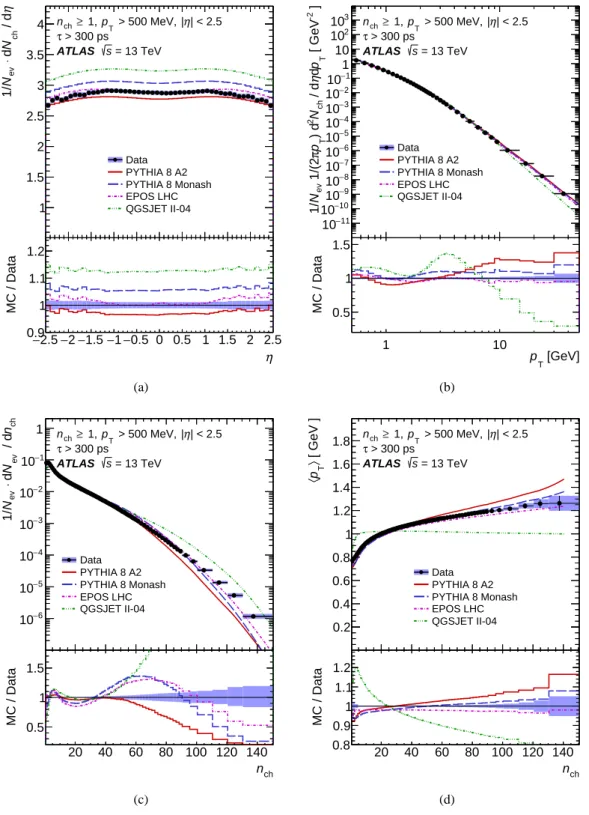
pT > 500 MeV and |η| < 2.5 are shown in Figure3. In most regions of all distributions the dominant uncertainty comes from the track reconstruction efficiency. The results are compared to predictions of models tuned to a wide range of measurements. The measured distributions are presented as inclusive distributions with corrections that rely minimally on the MC model used, in order to facilitate an accurate comparison with predictions.
Figure3(a)shows the multiplicity of charged particles as a function of pseudorapidity. The mean particle density is roughly constant at 2.9 for |η| < 1.0 and decreases at higher values of |η|. epos describes the data for |η| < 1.0, and predicts a slightly larger multiplicity at larger |η| values. qgsjet-ii and pythia8monash predict multiplicities that are too large by approximately 15% and 5% respectively. pythia8a2predicts a multiplicity that is 3% too low in the central region, but describes the data well in the forward region. Figure3(b)shows the charged-particle transverse momentum distribution. epos describes the data well over the entire pTspectrum. The pythia8tunes describe the data reasonably well, but are slightly above the data in the high-pT region. qgsjet-ii gives a poor prediction over the entire spectrum, overshooting the data in the low-pTregion and undershooting it in the high-pTregion.
Figure3(c)shows the charged-particle multiplicity distribution. The high-nch region has significant con-tributions from events with numerous MPI. pythia 8 a2 describes the data in the region nch < 50, but predicts too few events at larger nchvalues. pythia8monash, epos and qgsjet-ii describe the data reason-ably well in the region nch <30 but predict too many events in the mid-nch region, with pythia8monash and epos predicting too few events in the region nch > 100 while qgsjet-ii continues to be above the data.
Figure3(d)shows the mean transverse momentum versus the charged-particle multiplicity. The hpTi rises with nch, from 0.8 to 1.2 GeV. This increase is expected due to colour coherence effects being important in dense parton environments and is modelled by a colour reconnection mechanism in pythia 8 or by the hydrodynamical evolution model used in epos. If the high-nch region is assumed to be dominated by events with numerous MPI, without colour coherence effects the hpTi is approximately independent of
nch. Including colour coherence effects leads to fewer additional charged particles produced with every additional MPI, with an equally large pT to be shared among the produced hadrons [31]. epos predicts a slightly lower hpTi, but describes the dependence on nch very well. The pythia8tunes predict a steeper rise of hpTi with nch than the data, predicting lower values in the low-nchregion and higher values in the high-nch region. qgsjet-ii predicts a hpTi of ∼ 1 GeV, with very little dependence on nch; this is expected as it contains no model for colour coherence effects.
In summary, epos and the pythia8tunes describe the data most accurately, with epos reproducing the η and pTdistributions and the hpTi vs. nchthe best and pythia8a2describing the multiplicity the best in the low- and mid-nchregions. qgsjet-ii provides an inferior description of the data.
2.5 − −2−1.5−1−0.5 0 0.5 1 1.5 2 2.5 η / d ch N d ⋅ ev N 1/ 1 1.5 2 2.5 3 3.5 4 Data PYTHIA 8 A2 PYTHIA 8 Monash EPOS LHC QGSJET II-04 | < 2.5 η | > 500 MeV, T p 1, ≥ ch n > 300 ps τ = 13 TeV s ATLAS η 2.5 − −2−1.5−1−0.5 0 0.5 1 1.5 2 2.5 MC / Data 0.9 1 1.1 1.2 (a) ] -2 [ GeV T p d η / d ch N 2 ) d T p π 1/(2 ev N 1/ 11 − 10 10 − 10 9 − 10 8 − 10 7 − 10 6 − 10 5 − 10 4 − 10 3 − 10 2 − 10 1 − 10 1 10 2 10 3 10 Data PYTHIA 8 A2 PYTHIA 8 Monash EPOS LHC QGSJET II-04 | < 2.5 η | > 500 MeV, T p 1, ≥ ch n > 300 ps τ = 13 TeV s ATLAS [GeV] T p 1 10 MC / Data 0.5 1 1.5 (b) 20 40 60 80 100 120 140 ch n / d ev N d ⋅ ev N 1/ 6 − 10 5 − 10 4 − 10 3 − 10 2 − 10 1 − 10 1 Data PYTHIA 8 A2 PYTHIA 8 Monash EPOS LHC QGSJET II-04 | < 2.5 η | > 500 MeV, T p 1, ≥ ch n > 300 ps τ = 13 TeV s ATLAS ch n 20 40 60 80 100 120 140 MC / Data 0.5 1 1.5 (c) 20 40 60 80 100 120 140 [ GeV ] 〉 T p 〈 0.2 0.4 0.6 0.8 1 1.2 1.4 1.6 1.8 Data PYTHIA 8 A2 PYTHIA 8 Monash EPOS LHC QGSJET II-04 | < 2.5 η | > 500 MeV, T p 1, ≥ ch n > 300 ps τ = 13 TeV s ATLAS ch n 20 40 60 80 100 120 140 MC / Data 0.8 0.9 1 1.1 1.2 (d)
Figure 3: Primary-charged-particle multiplicities as a function of (a) pseudorapidity, η, and (b) transverse mo-mentum, pT; (c) the multiplicity, nch, distribution and (d) the mean transverse momentum, hpTi , versus nch in
events with nch ≥ 1, pT > 500 MeV and |η| < 2.5. The dots represent the data and the curves the predictions
from different MC models. The x-value in each bin corresponds to the bin centroid. The vertical bars represent the statistical uncertainties, while the shaded areas show statistical and systematic uncertainties added in quadrature. The bottom panel in each figure shows the ratio of the MC simulation to data. Since the bin centroid is different for data and simulation, the values of the ratio correspond to the averages of the bin content.
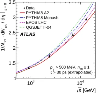
The mean number of primary charged particles in the central region is computed by averaging over |η| < 0.2 to be 2.874 ± 0.001 (stat.) ± 0.033 (syst.). This measurement is then corrected for the contribution from strange baryons and compared to previous measurements [1] at different √s values in Figure 4
together with the MC predictions. The correction factor for strange baryons depends on the MC model used and is found to be 1.0241 ± 0.0003 (epos), 1.0150 ± 0.0004 (pythia8monash) and 1.0151 ± 0.0002 (pythia8a2), where the uncertainties are statistical. qgsjet-ii does not include charged strange baryons. The prediction from epos is used to perform the extrapolation and the deviation from the pythia8monash prediction is taken as a systematic uncertainty and symmetrised to give 1.024 ± 0.009.
The mean number of primary charged particles increases by a factor of 2.2 when √s increases by a factor
of about 14 from 0.9 TeV to 13 TeV. epos and pythia8a2describe the dependence on √s very well, while pythia8monashand qgsjet-ii predict a steeper rise in multiplicity with √s.
[GeV] s 3 10 104 = 0 η η / d ch N d ⋅ ev N 1/ 1 1.5 2 2.5 3 3.5 1 ≥ ch n > 500 MeV, T p > 30 ps (extrapolated) τ ATLAS Data PYTHIA8 A2 PYTHIA8 Monash EPOS LHC QGSJET II-04
Figure 4: The average primary-charged-particle multiplicity in pp interactions per unit of pseudorapidity, η, for
|η| < 0.2 as a function of the centre-of-mass energy. The values at centre-of-mass energies other than 13 TeVare
taken from Ref. [1]. Charged strange baryons are included in the definition of primary particles. The data are compared to various particle-level MC predictions. The vertical error bars on the data represent the total uncertainty.
9. Conclusion
Primary-charged-particle multiplicity measurements with the ATLAS detector using proton–proton col-lisions delivered by the LHC at √s = 13 TeV are presented. From a data sample corresponding to an
integrated luminosity of 170 µb−1, nearly nine million inelastic interactions with at least one reconstruc-ted track with |η| < 2.5 and pT > 500 MeV are analysed. The results highlight clear differences between MC models and the measured distributions. Among the models considered epos reproduces the data the best, pythia8 a2 and monash give reasonable descriptions of the data and qgsjet-ii provides the worst description of the data.
Acknowledgements
We thank CERN for the very successful operation of the LHC, as well as the support staff from our institutions without whom ATLAS could not be operated efficiently.
We acknowledge the support of ANPCyT, Argentina; YerPhI, Armenia; ARC, Australia; BMWFW and FWF, Austria; ANAS, Azerbaijan; SSTC, Belarus; CNPq and FAPESP, Brazil; NSERC, NRC and CFI, Canada; CERN; CONICYT, Chile; CAS, MOST and NSFC, China; COLCIENCIAS, Colombia; MSMT CR, MPO CR and VSC CR, Czech Republic; DNRF, DNSRC and Lundbeck Foundation, Den-mark; IN2P3-CNRS, CEA-DSM/IRFU, France; GNSF, Georgia; BMBF, HGF, and MPG, Germany; GSRT, Greece; RGC, Hong Kong SAR, China; ISF, I-CORE and Benoziyo Center, Israel; INFN, Italy; MEXT and JSPS, Japan; CNRST, Morocco; FOM and NWO, Netherlands; RCN, Norway; MNiSW and NCN, Poland; FCT, Portugal; MNE/IFA, Romania; MES of Russia and NRC KI, Russian Feder-ation; JINR; MESTD, Serbia; MSSR, Slovakia; ARRS and MIZŠ, Slovenia; DST/NRF, South Africa; MINECO, Spain; SRC and Wallenberg Foundation, Sweden; SERI, SNSF and Cantons of Bern and Geneva, Switzerland; MOST, Taiwan; TAEK, Turkey; STFC, United Kingdom; DOE and NSF, United States of America. In addition, individual groups and members have received support from BCKDF, the Canada Council, CANARIE, CRC, Compute Canada, FQRNT, and the Ontario Innovation Trust, Canada; EPLANET, ERC, FP7, Horizon 2020 and Marie Skłodowska-Curie Actions, European Union; Investisse-ments d’Avenir Labex and Idex, ANR, Region Auvergne and Fondation Partager le Savoir, France; DFG and AvH Foundation, Germany; Herakleitos, Thales and Aristeia programmes co-financed by EU-ESF and the Greek NSRF; BSF, GIF and Minerva, Israel; BRF, Norway; the Royal Society and Leverhulme Trust, United Kingdom.
The crucial computing support from all WLCG partners is acknowledged gratefully, in particular from CERN and the ATLAS Tier-1 facilities at TRIUMF (Canada), NDGF (Denmark, Norway, Sweden), CC-IN2P3 (France), KIT/GridKA (Germany), INFN-CNAF (Italy), NL-T1 (Netherlands), PIC (Spain), ASGC (Taiwan), RAL (UK) and BNL (USA) and in the Tier-2 facilities worldwide.
References
[1] ATLAS Collaboration,
Charged-particle multiplicities in pp interactions measured with the ATLAS detector at the LHC, New J. Phys. 13 (2011) 053033, arXiv:1012.5104 [hep-ex].
[2] CMS Collaboration,
Charged particle multiplicities in pp interactions at √s = 0.9, 2.36, and 7 TeV,
JHEP 1101 (2011) 079, arXiv:1011.5531 [hep-ex].
[3] CMS Collaboration, Transverse momentum and pseudorapidity distributions of charged hadrons
in pp collisions at √s = 7 TeV,Phys. Rev. Lett. 105 (2010) 022002,
arXiv:1005.3299 [hep-ex].
[4] CMS Collaboration, Transverse momentum and pseudorapidity distributions of charged hadrons
in pp collisions at √s = 0.9 and 2.36 TeV,JHEP 1002 (2010) 041, arXiv:1002.0621 [hep-ex].
[5] ALICE Collaboration, K. Aamodt et al., Charged-particle multiplicity measured in proton-proton
collisions at √s = 7 TeV with ALICE at LHC,Eur. Phys. J. C 68 (2010) 345–354,
arXiv:1004.3514 [hep-ex].
[6] CDF Collaboration, T. Aaltonen et al., Measurement of Particle Production and Inclusive
Differential Cross Sections in p ¯p Collisions at √s =1.96 TeV,Phys. Rev. D 79 (2009) 112005,
arXiv:0904.1098 [hep-ex]. [7] CMS Collaboration,
Pseudorapidity distribution of charged hadrons in proton-proton collisions at √s = 13 TeV,
Phys. Lett. B 751 (2015) 143, arXiv:1507.05915 [hep-ex].
[8] ATLAS Collaboration, The ATLAS Experiment at the CERN Large Hadron Collider,
JINST 3 (2008) S08003.
[9] CMS Collaboration, The CMS experiment at the CERN LHC,JINST 3 (2008) S08004. [10] ALICE Collaboration, K. Aamodt et al., The ALICE experiment at the CERN LHC,
JINST 3 (2008) S08002.
[11] ATLAS Collaboration, ATLAS Insertable B-Layer Technical Design Report, CERN-LHCC-2010-013. ATLAS-TDR-19 (2010),
url:http://cdsweb.cern.ch/record/1291633,
CERN-LHCC-2012-009. ATLAS-TDR-19-ADD-1; ATLAS Collaboration,
ATLAS Insertable B-Layer Technical Design Report Addendum, CERN-LHCC-2012-009.
ATLAS-TDR-19-ADD-1 (2012), Addendum to CERN-LHCC-2010-013, ATLAS-TDR-019,
url:http://cdsweb.cern.ch/record/1451888.
[12] T. Sjöstrand, S. Mrenna and P. Z. Skands, A Brief Introduction to PYTHIA 8.1,
Comput. Phys. Commun. 178 (2008) 852, arXiv:0710.3820 [hep-ph]. [13] S. Porteboeuf, T. Pierog and K. Werner,
Producing Hard Processes Regarding the Complete Event: The EPOS Event Generator, (2010),
arXiv:1006.2967 [hep-ph]. [14] S. Ostapchenko,
Monte Carlo treatment of hadronic interactions in enhanced Pomeron scheme: QGSJET-II model, Phys. Rev. D 83 (2011) 014018, arXiv:1010.1869 [hep-ph].
[15] R. Corke and T. Sjöstrand, Interleaved parton showers and tuning prospects,
JHEP 1103 (2011) 032, arXiv:1011.1759.
[16] H. J. Drescher, M. Hladik, S. Ostapchenko, T. Pierog and K. Werner,
Parton-based Gribov–Regge theory,Phys. Rept. 350 (2001) 93,
arXiv:hep-ph/0007198 [hep-ph].
[17] V. N. Gribov, A Reggeon Diagram Technique, JETP 26 (1968) 414. [18] ATLAS Collaboration, Further ATLAS tunes of Pythia 6 and Pythia 8,
ATL-PHYS-PUB-2011-014, 2011, url:http://cds.cern.ch/record/1400677. [19] P. Skands, S. Carrazza and J. Rojo, Tuning PYTHIA 8.1: the Monash 2013 Tune,
Eur. Phys. J. C 74 (2014) 3024, arXiv:1404.5630 [hep-ph]. [20] T. Pierog, I. Karpenko, J. Katzy, E. Yatsenko and K. Werner,
EPOS LHC : test of collective hadronization with LHC data, (2013),
arXiv:1306.0121 [hep-ph].
[21] A. D. Martin, W. J. Stirling, R. S. Thorne and G. Watt, Parton distributions for the LHC,
Eur. Phys. J. C 63 (2009) 189, arXiv:0901.0002 [hep-ph].
[22] NNPDF Collaboration, R. D. Ball et al., Parton distributions with LHC data,
Nucl. Phys. B 867 (2013) 244, arXiv:1207.1303 [hep-ph].
[23] ATLAS Collaboration, The ATLAS Simulation Infrastructure,Eur. Phys. J. C 70 (2010) 823, arXiv:1005.4568 [physics.ins-det].
[24] GEANT4 Collaboration, S. Agostinelli et al., GEANT4 – A simulation toolkit, Nucl. Instr. Meth. A 506 (2003) 250.
[25] G. Piacquadio, K. Prokofiev and A. Wildauer,
Primary vertex reconstruction in the ATLAS experiment at LHC, J. Phys. Conf. Ser. 119 (2008) 032033.
[26] T. Cornelissen et al., Concepts, Design and Implementation of the ATLAS New Tracking (NEWT), ATL-SOFT-PUB-2007-007, 2007, url:http://cdsweb.cern.ch/record/1020106.
[27] T. Cornelissen et al., The new ATLAS track reconstruction (NEWT),
J. Phys. Conf. Ser. 119 (2008) 032014. [28] ATLAS Collaboration,
Track Reconstruction Performance of the ATLAS Inner Detector at √s = 13 TeV,
ATL-PHYS-PUB-2015-018, 2015, url:http://cds.cern.ch/record/2037683. [29] ATLAS Collaboration,
A study of the material in the ATLAS inner detector using secondary hadronic interactions, JINST 7 (2012) P01013, arXiv:1110.6191 [hep-ex].
[30] G. D’Agostini, A Multidimensional unfolding method based on Bayes’ theorem,
Nucl. Instr. Meth. A 362 (1995) 487–498.
[31] T. Sjöstrand, Colour reconnection and its effects on precise measurements at the LHC, (2013), arXiv:1310.8073 [hep-ph].
Appendix
A. Results in a common phase space
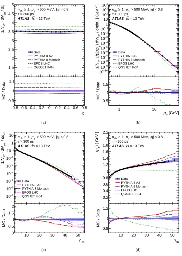
The corrected distributions for primary charged particles in events with nch ≥ 1 in the kinematic range
pT >500 MeV and |η| < 0.8 are shown in Figure5. This is the phase space that is common to the ATLAS, CMS and ALICE experiments.
The method used to correct the distributions and obtain the systematic uncertainties is exactly the same as that used for the results with |η| < 2.5, but obtained using the |η| < 0.8 selection.
Figure5(a) shows the primary-charged-particle multiplicity as a function of pseudorapidity, where the mean particle density is roughly 3.5, larger than in the main phase space due to the tighter restriction of at least one primary charged particle with |η| < 0.8. The pT and nch distributions are shown in Fig-ures5(b) and 5(c)respectively and the hpTi as a function of nch is shown in Figure 5(d). The level of agreement between the data and MC generator predictions follows the same pattern as seen in the main phase space.
0.8 − −0.6−0.4−0.2 0 0.2 0.4 0.6 0.8 η / d ch N d ⋅ ev N 1/ 1.5 2 2.5 3 3.5 4 4.5 5 Data PYTHIA 8 A2 PYTHIA 8 Monash EPOS LHC QGSJET II-04 | < 0.8 η | > 500 MeV, T p 1, ≥ ch n > 300 ps τ = 13 TeV s ATLAS η 0.8 − −0.6−0.4−0.2 0 0.2 0.4 0.6 0.8 MC / Data 0.9 1 1.1 (a) ] -2 [ GeV T p d η / d ch N 2 ) d T p π 1/(2 ev N 1/ 10 − 10 9 − 10 8 − 10 7 − 10 6 − 10 5 − 10 4 − 10 3 − 10 2 − 10 1 − 10 1 10 2 10 3 10 4 10 Data PYTHIA 8 A2 PYTHIA 8 Monash EPOS LHC QGSJET II-04 | < 0.8 η | > 500 MeV, T p 1, ≥ ch n > 300 ps τ = 13 TeV s ATLAS [GeV] T p 1 10 MC / Data 0.5 1 1.5 (b) 10 20 30 40 50 ch n / d ev N d ⋅ ev N 1/ 7 − 10 6 − 10 5 − 10 4 − 10 3 − 10 2 − 10 1 − 10 1 10 Data PYTHIA 8 A2 PYTHIA 8 Monash EPOS LHC QGSJET II-04 | < 0.8 η | > 500 MeV, T p 1, ≥ ch n > 300 ps τ = 13 TeV s ATLAS ch n 10 20 30 40 50 MC / Data 0 0.5 1 1.5 2 (c) 10 20 30 40 50 [ GeV ] 〉 T p 〈 0.2 0.4 0.6 0.8 1 1.2 1.4 1.6 1.8 2 2.2 Data PYTHIA 8 A2 PYTHIA 8 Monash EPOS LHC QGSJET II-04 | < 0.8 η | > 500 MeV, T p 1, ≥ ch n > 300 ps τ = 13 TeV s ATLAS ch n 10 20 30 40 50 MC / Data 0.8 1 1.2 (d)
Figure 5: Primary-charged-particle multiplicities as a function of (a) pseudorapidity, η, and (b) transverse mo-mentum, pT; (c) the multiplicity, nch, distribution and (d) the mean transverse momentum, hpTi , versus nch in
events with nch ≥ 1, pT >500 MeV and |η| < 0.8. The dots represent the data and the curves the predictions from
different MC models. The x-value in each bin corresponds to the bin centroid. The vertical bars represent the stat-istical uncertainties, while the shaded areas show statstat-istical and systematic uncertainties added in quadrature. The bottom panel in each figure shows the ratio of the MC simulation over the data. Since the bin centroid is different for data and simulation, the values of the ratio correspond to the averages of the bin content.
The ATLAS Collaboration
G. Aad86, B. Abbott113, J. Abdallah151, O. Abdinov11, B. Abeloos117, R. Aben107, M. Abolins91, O.S. AbouZeid137, N.L. Abraham149, H. Abramowicz153, H. Abreu152, R. Abreu116, Y. Abulaiti146a,146b, B.S. Acharya163a,163b ,a, L. Adamczyk39a, D.L. Adams26, J. Adelman108, S. Adomeit100, T. Adye131, A.A. Affolder75, T. Agatonovic-Jovin13, J. Agricola55, J.A. Aguilar-Saavedra126a,126f, S.P. Ahlen23, F. Ahmadov66,b, G. Aielli133a,133b, H. Akerstedt146a,146b, T.P.A. Åkesson82, A.V. Akimov96,
G.L. Alberghi21a,21b, J. Albert168, S. Albrand56, M.J. Alconada Verzini72, M. Aleksa31,
I.N. Aleksandrov66, C. Alexa27b, G. Alexander153, T. Alexopoulos10, M. Alhroob113, M. Aliev74a,74b, G. Alimonti92a, J. Alison32, S.P. Alkire36, B.M.M. Allbrooke149, B.W. Allen116, P.P. Allport18, A. Aloisio104a,104b, A. Alonso37, F. Alonso72, C. Alpigiani138, B. Alvarez Gonzalez31,
D. Álvarez Piqueras166, M.G. Alviggi104a,104b, B.T. Amadio15, K. Amako67, Y. Amaral Coutinho25a, C. Amelung24, D. Amidei90, S.P. Amor Dos Santos126a,126c, A. Amorim126a,126b, S. Amoroso31, N. Amram153, G. Amundsen24, C. Anastopoulos139, L.S. Ancu50, N. Andari108, T. Andeen32, C.F. Anders59b, G. Anders31, J.K. Anders75, K.J. Anderson32, A. Andreazza92a,92b, V. Andrei59a, S. Angelidakis9, I. Angelozzi107, P. Anger45, A. Angerami36, F. Anghinolfi31, A.V. Anisenkov109 ,c, N. Anjos12, A. Annovi124a,124b, M. Antonelli48, A. Antonov98, J. Antos144b, F. Anulli132a, M. Aoki67, L. Aperio Bella18, G. Arabidze91, Y. Arai67, J.P. Araque126a, A.T.H. Arce46, F.A. Arduh72, J-F. Arguin95, S. Argyropoulos64, M. Arik19a, A.J. Armbruster31, L.J. Armitage77, O. Arnaez31, H. Arnold49,
M. Arratia29, O. Arslan22, A. Artamonov97, G. Artoni120, S. Artz84, S. Asai155, N. Asbah43,
A. Ashkenazi153, B. Åsman146a,146b, L. Asquith149, K. Assamagan26, R. Astalos144a, M. Atkinson165, N.B. Atlay141, K. Augsten128, G. Avolio31, B. Axen15, M.K. Ayoub117, G. Azuelos95,d, M.A. Baak31, A.E. Baas59a, M.J. Baca18, H. Bachacou136, K. Bachas74a,74b, M. Backes31, M. Backhaus31,
P. Bagiacchi132a,132b, P. Bagnaia132a,132b, Y. Bai34a, J.T. Baines131, O.K. Baker175, E.M. Baldin109,c, P. Balek129, T. Balestri148, F. Balli136, W.K. Balunas122, E. Banas40, Sw. Banerjee172,e,
A.A.E. Bannoura174, L. Barak31, E.L. Barberio89, D. Barberis51a,51b, M. Barbero86, T. Barillari101, M. Barisonzi163a,163b, T. Barklow143, N. Barlow29, S.L. Barnes85, B.M. Barnett131, R.M. Barnett15, Z. Barnovska5, A. Baroncelli134a, G. Barone24, A.J. Barr120, L. Barranco Navarro166, F. Barreiro83, J. Barreiro Guimarães da Costa34a, R. Bartoldus143, A.E. Barton73, P. Bartos144a, A. Basalaev123, A. Bassalat117, A. Basye165, R.L. Bates54, S.J. Batista158, J.R. Batley29, M. Battaglia137,
M. Bauce132a,132b, F. Bauer136, H.S. Bawa143, f, J.B. Beacham111, M.D. Beattie73, T. Beau81, P.H. Beauchemin161, P. Bechtle22, H.P. Beck17,g, K. Becker120, M. Becker84, M. Beckingham169, C. Becot110, A.J. Beddall19e, A. Beddall19b, V.A. Bednyakov66, M. Bedognetti107, C.P. Bee148, L.J. Beemster107, T.A. Beermann31, M. Begel26, J.K. Behr43, C. Belanger-Champagne88, A.S. Bell79, W.H. Bell50, G. Bella153, L. Bellagamba21a, A. Bellerive30, M. Bellomo87, K. Belotskiy98,
O. Beltramello31, N.L. Belyaev98, O. Benary153, D. Benchekroun135a, M. Bender100, K. Bendtz146a,146b, N. Benekos10, Y. Benhammou153, E. Benhar Noccioli175, J. Benitez64, J.A. Benitez Garcia159b,
D.P. Benjamin46, J.R. Bensinger24, S. Bentvelsen107, L. Beresford120, M. Beretta48, D. Berge107, E. Bergeaas Kuutmann164, N. Berger5, F. Berghaus168, J. Beringer15, S. Berlendis56, N.R. Bernard87, C. Bernius110, F.U. Bernlochner22, T. Berry78, P. Berta129, C. Bertella84, G. Bertoli146a,146b,
F. Bertolucci124a,124b, I.A. Bertram73, C. Bertsche113, D. Bertsche113, G.J. Besjes37,
O. Bessidskaia Bylund146a,146b, M. Bessner43, N. Besson136, C. Betancourt49, S. Bethke101, A.J. Bevan77, W. Bhimji15, R.M. Bianchi125, L. Bianchini24, M. Bianco31, O. Biebel100,
D. Biedermann16, R. Bielski85, N.V. Biesuz124a,124b, M. Biglietti134a, J. Bilbao De Mendizabal50, H. Bilokon48, M. Bindi55, S. Binet117, A. Bingul19b, C. Bini132a,132b, S. Biondi21a,21b, D.M. Bjergaard46, C.W. Black150, J.E. Black143, K.M. Black23, D. Blackburn138, R.E. Blair6, J.-B. Blanchard136,
J.E. Blanco78, T. Blazek144a, I. Bloch43, C. Blocker24, W. Blum84,∗, U. Blumenschein55, S. Blunier33a, G.J. Bobbink107, V.S. Bobrovnikov109 ,c, S.S. Bocchetta82, A. Bocci46, C. Bock100, M. Boehler49, D. Boerner174, J.A. Bogaerts31, D. Bogavac13, A.G. Bogdanchikov109, C. Bohm146a, V. Boisvert78, T. Bold39a, V. Boldea27b, A.S. Boldyrev163a,163c, M. Bomben81, M. Bona77, M. Boonekamp136, A. Borisov130, G. Borissov73, J. Bortfeldt100, D. Bortoletto120, V. Bortolotto61a,61b,61c, K. Bos107, D. Boscherini21a, M. Bosman12, J.D. Bossio Sola28, J. Boudreau125, J. Bouffard2,
E.V. Bouhova-Thacker73, D. Boumediene35, C. Bourdarios117, S.K. Boutle54, A. Boveia31, J. Boyd31, I.R. Boyko66, J. Bracinik18, A. Brandt8, G. Brandt55, O. Brandt59a, U. Bratzler156, B. Brau87,
J.E. Brau116, H.M. Braun174,∗, W.D. Breaden Madden54, K. Brendlinger122, A.J. Brennan89,
L. Brenner107, R. Brenner164, S. Bressler171, T.M. Bristow47, D. Britton54, D. Britzger43, F.M. Brochu29, I. Brock22, R. Brock91, G. Brooijmans36, T. Brooks78, W.K. Brooks33b, J. Brosamer15, E. Brost116, J.H Broughton18, P.A. Bruckman de Renstrom40, D. Bruncko144b, R. Bruneliere49, A. Bruni21a, G. Bruni21a, BH Brunt29, M. Bruschi21a, N. Bruscino22, P. Bryant32, L. Bryngemark82, T. Buanes14, Q. Buat142, P. Buchholz141, A.G. Buckley54, I.A. Budagov66, F. Buehrer49, M.K. Bugge119,
O. Bulekov98, D. Bullock8, H. Burckhart31, S. Burdin75, C.D. Burgard49, B. Burghgrave108, K. Burka40, S. Burke131, I. Burmeister44, E. Busato35, D. Büscher49, V. Büscher84, P. Bussey54, J.M. Butler23, A.I. Butt3, C.M. Buttar54, J.M. Butterworth79, P. Butti107, W. Buttinger26, A. Buzatu54,
A.R. Buzykaev109 ,c, S. Cabrera Urbán166, D. Caforio128, V.M. Cairo38a,38b, O. Cakir4a, N. Calace50, P. Calafiura15, A. Calandri86, G. Calderini81, P. Calfayan100, L.P. Caloba25a, D. Calvet35, S. Calvet35, T.P. Calvet86, R. Camacho Toro32, S. Camarda31, P. Camarri133a,133b, D. Cameron119,
R. Caminal Armadans165, C. Camincher56, S. Campana31, M. Campanelli79, A. Campoverde148, V. Canale104a,104b, A. Canepa159a, M. Cano Bret34e, J. Cantero83, R. Cantrill126a, T. Cao41,
M.D.M. Capeans Garrido31, I. Caprini27b, M. Caprini27b, M. Capua38a,38b, R. Caputo84, R.M. Carbone36, R. Cardarelli133a, F. Cardillo49, T. Carli31, G. Carlino104a, L. Carminati92a,92b, S. Caron106,
E. Carquin33b, G.D. Carrillo-Montoya31, J.R. Carter29, J. Carvalho126a,126c, D. Casadei18, M.P. Casado12 ,h, M. Casolino12, D.W. Casper162, E. Castaneda-Miranda145a, A. Castelli107,
V. Castillo Gimenez166, N.F. Castro126a ,i, A. Catinaccio31, J.R. Catmore119, A. Cattai31, J. Caudron84, V. Cavaliere165, E. Cavallaro12, D. Cavalli92a, M. Cavalli-Sforza12, V. Cavasinni124a,124b,
F. Ceradini134a,134b, L. Cerda Alberich166, B.C. Cerio46, A.S. Cerqueira25b, A. Cerri149, L. Cerrito77, F. Cerutti15, M. Cerv31, A. Cervelli17, S.A. Cetin19d, A. Chafaq135a, D. Chakraborty108,
I. Chalupkova129, S.K. Chan58, Y.L. Chan61a, P. Chang165, J.D. Chapman29, D.G. Charlton18,
A. Chatterjee50, C.C. Chau158, C.A. Chavez Barajas149, S. Che111, S. Cheatham73, A. Chegwidden91, S. Chekanov6, S.V. Chekulaev159a, G.A. Chelkov66 , j, M.A. Chelstowska90, C. Chen65, H. Chen26, K. Chen148, S. Chen34c, S. Chen155, X. Chen34f, Y. Chen68, H.C. Cheng90, H.J Cheng34a, Y. Cheng32, A. Cheplakov66, E. Cheremushkina130, R. Cherkaoui El Moursli135e, V. Chernyatin26 ,∗, E. Cheu7, L. Chevalier136, V. Chiarella48, G. Chiarelli124a,124b, G. Chiodini74a, A.S. Chisholm18, A. Chitan27b, M.V. Chizhov66, K. Choi62, A.R. Chomont35, S. Chouridou9, B.K.B. Chow100, V. Christodoulou79, D. Chromek-Burckhart31, J. Chudoba127, A.J. Chuinard88, J.J. Chwastowski40, L. Chytka115,
G. Ciapetti132a,132b, A.K. Ciftci4a, D. Cinca54, V. Cindro76, I.A. Cioara22, A. Ciocio15, F. Cirotto104a,104b, Z.H. Citron171, M. Ciubancan27b, A. Clark50, B.L. Clark58, M.R. Clark36, P.J. Clark47, R.N. Clarke15, C. Clement146a,146b, Y. Coadou86, M. Cobal163a,163c, A. Coccaro50, J. Cochran65, L. Coffey24,
L. Colasurdo106, B. Cole36, S. Cole108, A.P. Colijn107, J. Collot56, T. Colombo31, G. Compostella101, P. Conde Muiño126a,126b, E. Coniavitis49, S.H. Connell145b, I.A. Connelly78, V. Consorti49,
S. Constantinescu27b, C. Conta121a,121b, G. Conti31, F. Conventi104a ,k, M. Cooke15, B.D. Cooper79, A.M. Cooper-Sarkar120, T. Cornelissen174, M. Corradi132a,132b, F. Corriveau88,l, A. Corso-Radu162, A. Cortes-Gonzalez12, G. Cortiana101, G. Costa92a, M.J. Costa166, D. Costanzo139, G. Cottin29,
W.A. Cribbs146a,146b, M. Crispin Ortuzar120, M. Cristinziani22, V. Croft106, G. Crosetti38a,38b, T. Cuhadar Donszelmann139, J. Cummings175, M. Curatolo48, J. Cúth84, C. Cuthbert150, H. Czirr141, P. Czodrowski3, S. D’Auria54, M. D’Onofrio75, M.J. Da Cunha Sargedas De Sousa126a,126b, C. Da Via85, W. Dabrowski39a, T. Dai90, O. Dale14, F. Dallaire95, C. Dallapiccola87, M. Dam37, J.R. Dandoy32, N.P. Dang49, A.C. Daniells18, N.S. Dann85, M. Danninger167, M. Dano Hoffmann136, V. Dao49, G. Darbo51a, S. Darmora8, J. Dassoulas3, A. Dattagupta62, W. Davey22, C. David168, T. Davidek129, M. Davies153, P. Davison79, Y. Davygora59a, E. Dawe89, I. Dawson139, R.K. Daya-Ishmukhametova87, K. De8, R. de Asmundis104a, A. De Benedetti113, S. De Castro21a,21b, S. De Cecco81, N. De Groot106, P. de Jong107, H. De la Torre83, F. De Lorenzi65, D. De Pedis132a, A. De Salvo132a, U. De Sanctis149, A. De Santo149, J.B. De Vivie De Regie117, W.J. Dearnaley73, R. Debbe26, C. Debenedetti137, D.V. Dedovich66, I. Deigaard107, J. Del Peso83, T. Del Prete124a,124b, D. Delgove117, F. Deliot136, C.M. Delitzsch50, M. Deliyergiyev76, A. Dell’Acqua31, L. Dell’Asta23, M. Dell’Orso124a,124b,
M. Della Pietra104a,k, D. della Volpe50, M. Delmastro5, P.A. Delsart56, C. Deluca107, D.A. DeMarco158, S. Demers175, M. Demichev66, A. Demilly81, S.P. Denisov130, D. Denysiuk136, D. Derendarz40, J.E. Derkaoui135d, F. Derue81, P. Dervan75, K. Desch22, C. Deterre43, K. Dette44, P.O. Deviveiros31, A. Dewhurst131, S. Dhaliwal24, A. Di Ciaccio133a,133b, L. Di Ciaccio5, W.K. Di Clemente122,
A. Di Domenico132a,132b, C. Di Donato132a,132b, A. Di Girolamo31, B. Di Girolamo31, A. Di Mattia152, B. Di Micco134a,134b, R. Di Nardo48, A. Di Simone49, R. Di Sipio158, D. Di Valentino30, C. Diaconu86, M. Diamond158, F.A. Dias47, M.A. Diaz33a, E.B. Diehl90, J. Dietrich16, S. Diglio86, A. Dimitrievska13, J. Dingfelder22, P. Dita27b, S. Dita27b, F. Dittus31, F. Djama86, T. Djobava52b, J.I. Djuvsland59a,
M.A.B. do Vale25c, D. Dobos31, M. Dobre27b, C. Doglioni82, T. Dohmae155, J. Dolejsi129, Z. Dolezal129, B.A. Dolgoshein98 ,∗, M. Donadelli25d, S. Donati124a,124b, P. Dondero121a,121b, J. Donini35, J. Dopke131, A. Doria104a, M.T. Dova72, A.T. Doyle54, E. Drechsler55, M. Dris10, Y. Du34d, J. Duarte-Campderros153, E. Duchovni171, G. Duckeck100, O.A. Ducu27b, D. Duda107, A. Dudarev31, L. Duflot117, L. Duguid78, M. Dührssen31, M. Dunford59a, H. Duran Yildiz4a, M. Düren53, A. Durglishvili52b, D. Duschinger45, B. Dutta43, M. Dyndal39a, C. Eckardt43, K.M. Ecker101, R.C. Edgar90, W. Edson2, N.C. Edwards47, T. Eifert31, G. Eigen14, K. Einsweiler15, T. Ekelof164, M. El Kacimi135c, V. Ellajosyula86, M. Ellert164, S. Elles5, F. Ellinghaus174, A.A. Elliot168, N. Ellis31, J. Elmsheuser26, M. Elsing31, D. Emeliyanov131, Y. Enari155, O.C. Endner84, M. Endo118, J.S. Ennis169, J. Erdmann44, A. Ereditato17, G. Ernis174, J. Ernst2, M. Ernst26, S. Errede165, E. Ertel84, M. Escalier117, H. Esch44, C. Escobar125, B. Esposito48, A.I. Etienvre136, E. Etzion153, H. Evans62, A. Ezhilov123, F. Fabbri21a,21b, L. Fabbri21a,21b, G. Facini32, R.M. Fakhrutdinov130, S. Falciano132a, R.J. Falla79, J. Faltova129, Y. Fang34a, M. Fanti92a,92b, A. Farbin8, A. Farilla134a, C. Farina125, T. Farooque12, S. Farrell15, S.M. Farrington169, P. Farthouat31, F. Fassi135e, P. Fassnacht31, D. Fassouliotis9, M. Faucci Giannelli78, A. Favareto51a,51b, W.J. Fawcett120, L. Fayard117, O.L. Fedin123,m, W. Fedorko167, S. Feigl119, L. Feligioni86, C. Feng34d, E.J. Feng31, H. Feng90,
A.B. Fenyuk130, L. Feremenga8, P. Fernandez Martinez166, S. Fernandez Perez12, J. Ferrando54, A. Ferrari164, P. Ferrari107, R. Ferrari121a, D.E. Ferreira de Lima54, A. Ferrer166, D. Ferrere50, C. Ferretti90, A. Ferretto Parodi51a,51b, F. Fiedler84, A. Filipˇciˇc76, M. Filipuzzi43, F. Filthaut106, M. Fincke-Keeler168, K.D. Finelli150, M.C.N. Fiolhais126a,126c, L. Fiorini166, A. Firan41, A. Fischer2, C. Fischer12, J. Fischer174, W.C. Fisher91, N. Flaschel43, I. Fleck141, P. Fleischmann90, G.T. Fletcher139, G. Fletcher77, R.R.M. Fletcher122, T. Flick174, A. Floderus82, L.R. Flores Castillo61a,
M.J. Flowerdew101, G.T. Forcolin85, A. Formica136, A. Forti85, A.G. Foster18, D. Fournier117, H. Fox73, S. Fracchia12, P. Francavilla81, M. Franchini21a,21b, D. Francis31, L. Franconi119, M. Franklin58,
M. Frate162, M. Fraternali121a,121b, D. Freeborn79, S.M. Fressard-Batraneanu31, F. Friedrich45, D. Froidevaux31, J.A. Frost120, C. Fukunaga156, E. Fullana Torregrosa84, T. Fusayasu102, J. Fuster166, C. Gabaldon56, O. Gabizon174, A. Gabrielli21a,21b, A. Gabrielli15, G.P. Gach39a, S. Gadatsch31, S. Gadomski50, G. Gagliardi51a,51b, L.G. Gagnon95, P. Gagnon62, C. Galea106, B. Galhardo126a,126c,