In how much is REN worth, indeed?
Equity Research
Redes Energéticas Nacionais, SPGS, SA
Marta Almeida Coimbra Casqueiro, 152112337
"
Don't gamble. Take all your money, buy a good stock and hold it until
it goes up, then sell it. If it doesn't go up, don't buy it"- Will Rogers
Advisor: José Carlos Tudela Martins
Dissertation submitted in partial fulfillment of requirements for the degree of
MSC in Business Administration at Catolica Lisbon School of Business and
Economics
Abstract
For the last years, different authors and scholars have been focusing their studies on firm valuation. Despite the fact that this subject is, to a somewhat large extent, a matter of some controversy, almost all of the discussions agree on the point that valuing a company is an art.
Hereupon, this dissertation aims to present an equity valuation anchored on this idea, for which purpose attempting to combine the review of significant literature and studies with the valuation of a Portuguese operator of electricity and natural gas networks, Redes Energéticas Nacionais, S.A. (REN).
Hence, this study proposes a price target for the company’s stock between 3.14 and 3.39 Euros, the 31st of March 2014 being the reference date for such valuation. Banco Portguês de Investimento’s research is additionally offered as a basis for comparison, both as to methodologies followed and results obtained.
Acknowledgments
I would like to express my sincere gratitude to Professor José Carlos Tudela Martins for the prompt and kind guidance and helpful feedback as well as for his availability. I would also like to thank the equity analyst Gonzalo Sanchez Bordona from Banco Português de Investimentos for the important recommendations, which much contributed to improve the work.
On the other hand, a word of recognition to Marta Carvalho, Carlota Casqueiro and Diogo Casqueiro for their support and aid in revising the English of the dissertation.
Finally, I would like to convey my profound gratitude and love to my family, for everything that I will never be able to express in words, friends and to Frederico Carvalho. A distinctive recognition to my mother, Ana Casqueiro, who provided a great support during all my studies, principally in the most difficult times.
A special word, however, is due to my father, Carlos Casqueiro, to whom I dedicate this dissertation, because of his unlimited help, his invaluable knowledge and the expertise he conveyed. Thank you for all the financial knowledge given and the patience demonstrated. I will always remember it fondly and I will always be in your debt for teaching me that “Valuing a company is an art”.
Index
A.
Executive Summary ... 4
I.
Object of the Thesis ... 5
II.
Organization of the Work ... 5
III.
Main Conclusions ... 5
B.
Valuation Methodologies ... 9
I.
Firms’ Value and Valuation Models ... 10
II.
Income Method ... 11
III.
Market Comparable Method ... 33
IV.
Other Valuation Methods ... 38
V.
REN Group Valuation Methods and Parameters ... 39
C.
Brief Description of REN Group ... 46
I.
Information about REN Group ... 47
II.
Information on REN Group’s Business Areas ... 49
III.
Recent Performance of REN Group and Conclusions ... 57
D.
REN Group Valuation ... 63
I.
Valuation Preparation... 64
II.
REN’s Prefiguration of Provisional Activity ... 65
III.
Discounted Cash Flow Method ... 77
IV.
Valuation Comparison ... 81
V.
Market Multiples Method ... 84
I.
Object of the Thesis
The object of this thesis is to determine the share value of REN - Redes Energéticas Nacionais SGPS, SA (REN or the Company and jointly with its subsidiaries designated by REN Group or Group) as reported on December 31st 2013.
II.
Organization of the Work
According to the object of this thesis, the work is divided into the following stages:
1. A succinct description of the companies’ evaluation methodologies, its main characteristics and its main merits and fragilities (Chapter B). This stage of the work concludes with the presentation of the methodologies which were applied in the evaluation of REN Group and of a series of parameters essential to its achievement;
2. A short characterization of REN Group, essential for analyzing its projected business and also for selecting the evaluation methods to be applied (Chapter C); and
3. Evaluation of REN Group, taking into account all the available information and conclusions drawn from the analysis carried out (Chapter D).
This document finishes with the presentation of the main bibliography sources used in the elaboration of this thesis.
III.
Main Conclusions
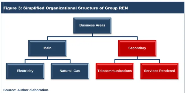
The analysis shows that REN Group is the major entity in the national electricity and natural gas market, where it operates under concession contracts granted by the Portuguese state, and subject to economic regulation models, the aim of which is to mitigate market flaws associated with activities of great capital intensity, which are therefore performed in non-competitive conditions.
Additionally, REN Group also operates in the telecommunications sector, renting the fiber installed in its electrical gas system infrastructures.
The analysis of REN Group‘s recent evolution enables to conclude:
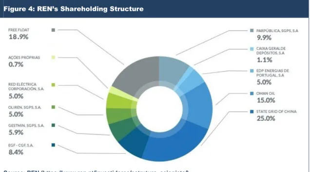
1. That its shareholder basis is quite concentrated, with a free-float below 19%;
2. That its business is relatively small when compared with its European peers, with a firm market value of 4,012 million Euros, according to Bloomberg;
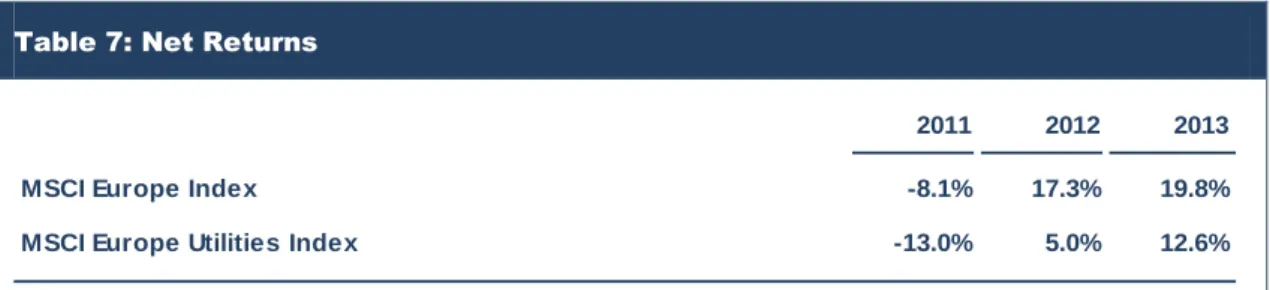
3. That in the last three years, its levels of returns (average ROE of 11.8%) were markedly less than its peers (18.4% of sector average);
4. That it has an aggressive capital structure and a lower financial flexibility level than all its peers, and thus the reason for being given a non-investment grade rating notation; and
5. That it is subject not only to significant regulatory risks, as regulation periods only have a 3-year duration, but also to political risks as seen in 2014 with the levying of an extraordinary contribution rate on the energy sector.
Based on these circumstances, REN’s stocks have been traded with a discount, in relation to its European peers: around 13%, based on firm values to EBITDA ratios; and close to 3%, based on PE multiples.
With the aim of determining the value of REN Group based on discounted cash flows methods and market multiples, a projection of its estimated business was carried out and the following scenario was assumed:
Electricity Natural Gas
1. End of concession period (year) 2057 2046
2. Regulated Asset Base
a. Value (31 December 2013)
b. Annual average Capex (2013 prices)
c. Annual average depreciations (2013 prices)
2,419 Mn € 213 Mn € 268 Mn € 1,112 Mn € 51 Mn € 77 Mn €
Electricity Natural Gas 3. Operating expenses
a. Value (2013)
b. Real Variation(Annual average Δ consumption)
67 Mn €
1.0%
38 Mn €
2.2%
4. Operating Income
a. Average rate of return of remuneration of the RAB
b. Annual average depreciations (2013 prices)
c. Other revenues (weight on capital revenue)
d. Own Works (weight on Capex)
5.8% 268 Mn € 1.1% 9.5% 6.0% 77 Mn € 2.3% 9.1%
The evaluation undertaken with basis on the market information reported at March 31st 2014, showed that the value of the stocks of REN Group are the following:
The current price of REN Group‘s stocks embodies a discount of around 13% in relation to the central point of the interval of value inferred for its stocks (3.27 Euros) and market analysts’ average price target ( 2.56 Euros) have an underlying discount of around 12%.
The reason for these differentials lies apparently in three fundamental factors:
1. Firstly, investors and analysts’ fear that the extraordinary tax levied on the energy sector in 2014 will continue in the future;
Valuation
Max €
3.39
Min €
3.14
Price
2.86 €
Price
Targets
Max
2.90 €
Min
2.22 €
2. Secondly, the minute share free-float ( limited to 18.9%) that leads them to apply an illiquidity discount; and
3. Thirdly, the existing pressure on the share price as result of the privatization operation involving 11% of its capital still held by the State, planned for the summer 2014.
The Government has already said that it will not keep the extraordinary tax on energy, beyond 2014, and that the sale of an additional 11% of REN’s capital will determine an increase of its free-float to roughly 30% and consequently to an increase in the liquidity level of its shares.
In this context, taking into account the prevailing conditions in the capital markets, the characteristics of
REN Group and all the available information, it is reasonable to consider that the current value of its shares is somewhere between 3.14 and 3.39 Euros.
I.
Firms’ Value and Valuation Models
1.
Firms’ Value
The value of a company, also referred to as enterprise value or firm value, may be defined as the amount by which the net assets of the company (or the capitals invested in the company) may be traded between independent entities who are reasonably informed about the characteristics of that company
VL = E + D (1)
As such, the value of a company (VL) may be defined as the sum of the market values of its equity
capital or equity value (E) and that of its net debt (D), in the case where the net assets are financed only with equity capital and debt.
The lenders or financial creditors become holders of the value of the loans granted to the company while equity holders are granted the residual value, i.e., the difference between the market value of the firm and the value of its net debt.
2.
Valuation Model Families
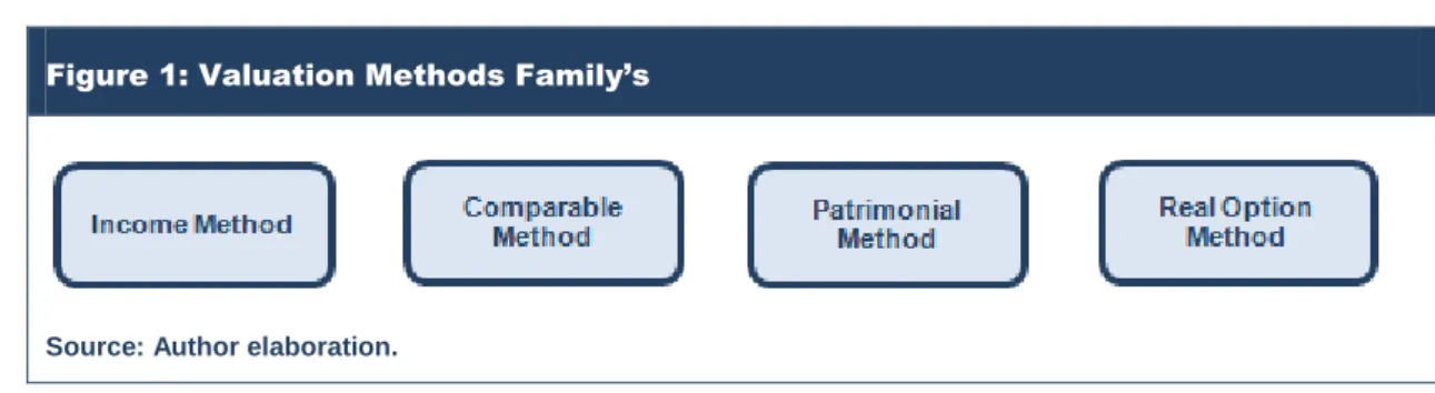
Company valuation models can be classified into four major families.
Figure 1: Valuation Methods Family’s
Source: Author elaboration.
The most widely used valuation models are the ones grouped within the income method and the comparable method. The patrimonial approach has its field of action relatively limited to the determination of companies’ liquidation value and the real options method, notwithstanding its technical merits, is still not very widely used.
Each of the aforementioned methods may be applied with the objective of determining the value of a firm or the value of its equity.
II.
Income Method
1.
Introduction
The income method is based on the principle that the value of a financial asset is equivalent to the value of future returns expected to be generated, discounted with reference to the evaluation date at a rate that adequately reflects the prevailing financial market conditions and the level of risk associated with those future returns.
According to this method of valuation, the value of a company can be determined in various alternative ways, namely:
1. The present value approach or the adjusted rate of return approach;
2. The adjusted present value approach;
3. The capital cash flow approach;
4. The economic value added approach;
5. The dividend discount model approach;
6. The flow to equity approach;
7. The residual income approach.
The objective of the approaches indicated in the first four paragraphs above is to firstly to determine the value of companies and then, the value of their equity capital. As for the last three above-mentioned approaches, their purpose is to directly identify the value of a company’s equity capital.
2.
Present Value Approach
2.1. Conceptualization
In the present value approach the company’s value is determined through the update, with regard to the reference valuation date, (i) of the expected free cash flow series (FCF) at (ii) a discount rate usually
referred to as weighted average cost of capital (RW), which can also be referred to as adjusted rate of return.
n 1 t W t t L (1FCFR ) V (2)In accordance with this approach, the company value is calculated with basis on the expression contained in (2) above, in which the variable n represents the economic life of the company.
2.2. Expected Free Cash Flows
Free cash flows are a measure that translates the firms’ assets’ (or businesses) expected fund generating capacity and, consequently, the capacity of the available funds to remunerate every capital provider.
One way of determining the company’s free cash flows is the following:
FCF = EBIT x (1 – TC) + D&A – Capex – Δ WK (3)
In which:
EBIT = Earnings before interest and taxes;
TC = Marginal tax rate on the income of the company;
D&A = Depreciations and amortizations;
Capex = Investments in fixed assets; Δ WK = Variation in working capital.
The product between operational results (EBIT) and the additional value to the marginal tax rate on corporate income (1-TC) corresponds to the operational results after taxes, usually referred to as NOPLAT.
The difference between depreciations and amortizations (D&A) and investment in fixed assets (Capex) and in net working capital (Δ WK) corresponds to the variation of the invested capital in the businesses of the firm and this measure can be designated as Δ K.
Accordingly, free cash flows may also be expressed in the following manner:
FCF = NOPLAT – Δ K (4)
At this point it is important to emphasize that the free cash flows are future flows, not observable, and as such, constitute an expected amount (uncertain) and is associated with a certain risk level.
2.3. Weighted Average Cost of Capital
The weighted average cost of capital (RW) is a rate of return that intends to translate the net return that
the assets (or businesses) of a company should generate, so that the company can adequately remunerate all capital invested in it.
So, in its broader formulation, the weighted average cost of capital can be expressed in the following manner:
n 1 i i i W R xW R (5) In which:RI = Net rate of return demanded by investors who provide class i capital used by the
company;
WI = Class i capital weight in the company’s funding structure; and
n = Number of capital classes used by the company.
In a more restrictive formulation, in which the companies’ businesses are financed only through debt and own capitals, the weighted average cost of capital can be expressed in the following manner:
RW = RD x (1 – TC) x L + RE x (1 – L) (6)
RD = Expected cost of debt of the company;
RE = Expected cost of equity of the company;
L = Debt burden of the company in its funding structure.
The weight of each financing source (or of class of capital) used by the company is quantified in market values and not in book values.
The weighted average cost of capital is an adjusted return rate, insofar as it does not reflect the return that should be generated by the company’s assets but the profitability rate that those assets can generate, taking into account the way they are financed.
3.
Adjusted Present Value Approach
3.1. Conceptualization
In the adjusted present value approach it is explicitly recognized that a company’s value is not only a function of the income flows generated by the assets (free cash flows) but also a function of the benefits and drawbacks determined by the debt used in its financing.
Accordingly, a company’s value (VL) is calculated with basis on the sum of the value that such company
would hold if it was entirely financed by equity capitals (VU) and the difference between the benefit
values (BD) and the drawbacks (MD) induced by the debt:
VL = VU + BD – MD (7)
Hence, according to the adjusted present value approach, in order to determine a company’s value it is necessary to identify three relevant income flows and three relevant return rates.
3.2. Base Value of the Assets
The first relevant income flow corresponds to the expected free cash flows and the current value of this series of flows (base value of the assets) is determined by discounting it at a return rate designated by opportunity cost of capital (RU):
n 1 t U t t U (1FCFR ) V (8)Conventionally, companies will only become indebted as long as that decision creates value and, because of that, the value of a company which is not in debt will always tend to be equal or inferior to the value of that company with debt, and thus the reason why the capital’s opportunity cost is higher than or equal to the capital weighted average cost of capital (RU≥ RW)1.
3.3. Value of the Debt-Induced Benefits
The main benefit induced by the use of debt in the funding of companies’ businesses, lies among others in tax savings (or tax shields) which can be obtained from loan interests2.
The tax shields value (TSD) corresponds to the product between the amounts of contracted debt (D), the
gross cost of that debt (RD) and the marginal tax rate on the company’s income (TC):
TSD = D x RD x TC (9)
The return rate (RTSD) at which the tax shields may be discounted in order to determine their present
value is quite a controversial issue among financial experts, lying somewhere between the gross debt cost (RD) and the capital’s opportunity cost (RU).
In general, it is normal to consider that, if the amount of debt owned by a company is independent from its businesses’ values, then the tax shields’ risk is equally independent from the free cash flows’ risk and tends to be equivalent to the debt’s risk. In this case, the appropriate discount rate to ascertain the present value of the benefits induced by debt corresponds to the gross cost of debt:
n 1 t Dt t SD D ) R 1 ( T B (10.a) 1Capital opportunity cost equals the weighted average cost of capital in cases where the company does not resort to debt to finance its business.
2
Among the remaining benefits induced by the use of debt, the most relevant is probably the adoption of a more rigorous management.
In the event that the amount of debt held by a company is periodically defined according to its businesses’ value, then the risk associated with the tax shields is equivalent to that of the free cash flows and, consequently, the appropriate rate to determine its present value is, in the first period, the gross debt cost and, in the subsequent periods, the capital opportunity cost.
In this case, the value of the benefits induced by the use of debt is determined using the following formula: D U n 1 t Ut t SD D (1TR ) x11 RR B
(10.b)3.4. Value of Debt-related Drawbacks
If it is true that indebtedness generates economic benefits for companies, it is likewise true that resorting to debt also causes problems in terms of: (i) bankruptcy costs; (ii) agency costs (between shareholders and debt holders); and (iii) loss of financial flexibility.
Focusing the analysis on bankruptcy cost (or of financial distress), it is possible to observe that these encumbrances involve two different aspects: (i) one respecting direct costs (namely, legal and administrative costs); and (ii) another relating to indirect costs, resulting from the perception that bankruptcy is likely, whether by clients, suppliers’ employees, or by the funding entities themselves.
Conceptually, the ex-ante value of the financial distress costs is equivalent to the product between the default probability (PD) and the ex-post value of the financial distress costs.
Unfortunately, neither the bankruptcy’s probability nor the ex-post value of the bankruptcy’s costs are parameters subject to direct estimate, reason why the estimate concerning the value of the damage induced by indebtedness constitutes a field of intense debate among financial specialists and in relation to which sufficiently reliable and robust conclusions are yet to be reached.
In any event, taking a study3 published in the Journal of Applied Corporate Finance into account, the
ex-ante value of the bankruptcy’s costs tends to represent the following percentages of companies’ market values:
3 “
Chart 1: EX-Ante Value of Bankruptcy Costs by Rating Classes
Source: Estimating Risk-Adjusted Costs of Financial Distress.
As should be expected, the lower the credit qualities of the company and, therefore, their rating notations, the higher the expected values of the financial distress costs.
4.
Other Alternative Approaches
4.1. Capital Cash Flow Approach
In the capital cash flow approach, the relevant variables in determining the company’s value are: (i) the expected capital cash flows; and (ii) the weighted average cost of capital before taxes.
The capital cash flows (CCF) correspond to the sum of the free cash flows with the tax shields:
CCF = EBIT x (1 – TC) + D&A – Capex – Δ WK + D x RD x TC (11)
In its turn, the weighted average cost of capital before taxes (RWST) is represented by the following
expression:
RWBT = RD x L + RE x (1 – L) (12)
4.2. Economic Value Added Approach
The economic value added (EVA) is a measure that quantifies the additional return that the company’s business generates in relation to the weighted average cost of capital:
0.6% 1.9%
3.4% 5.1%
7.8%
10.0%
EVA = NOPLAT – K x RW EVA = K x (ROIC4 – RW) (13)
Thus, according to the economic value added approach, a company’s value can be determined using the following expression:
n 1 t W t t L K (1EVAR ) V (14)4.3. Dividends Approach
According to the dividends approach, the value of the equity capital of a company is determined by discounting, to the reference valuation date, the expected flow of dividends of that company (DIV) at a rate which reflects the costs of its equity capital (RE):
n 1 t E t t ) R 1 ( DIV E (15)If, afterwards, ascertaining the company’s value is intended, then it is only necessary to add the equity value to the company´s debt value, as shown in the expression (1) above.
4.4. Flow to Equity Approach
In the flow to equity approach, the relevant variables for determining the equity value are the equity cash flows (ECF) and the cost of the equity capital (RE).
The equity cash flows correspond to the difference between the cash flows and the debt cash flows (DCF), which represent the portion of the free cash flows subject to appropriation by lenders:
DCF = D x RD x (1 – TC) – Δ D (16)
Thereby, the equity cash flows are obtained using the following expression:
ECF = FCF – DCF = EBIT x (1 – TC) + D&A – Capex – Δ WK – D x RD x (1 – TC) + Δ D (17)
4
In the long run, the value of the dividend series and the value of the equity cash flows generated by the companies have to be, necessarily, identical.
4.5. Residual Income Approach
The residual income (RI) is a measure that quantifies the extra return that the equity capitals (CP) of a company generate in relation to its cost of capital:
RI = Net Income – CP x RE RI = CP x (ROE5 – RE) (18)
This way, according to the residual income approach, a company’s equity value can be determined by the following expression:
n 1 t E t t ) R 1 ( RI CP E (19)5.
Cost of Capital
5.1. Conceptualization
The cost of capital of a financial asset corresponds to the rate of returns (R) presumably demanded by investors for acquiring that title. And, according to the financial theory, investors establish that expected return rate basing their expectations on: (i) the remuneration rate offered by risk free financial assets (RF); and (ii) the level of risk associated with the asset (PR).
In these terms, the return rate that the rational economic agents will tend to demand to invest on a financial asset can be expressed as the sum of the two above-mentioned measures:
R = RF + PR (20)
This is the basic notion of capital cost, common to all the developed models with the purpose of determining this referential: the cost of capital is the function of the rate of return offered by the risk free
5
assets and the investors’ perception of the risk level subjacent to the specific asset in which they are planning to invest.
5.2. Capital Asset Pricing Model
There are several models used to determine the cost of capital of financial assets. The most used one, however, is the Capital Asset Pricing Model (CAPM)6, originally proposed by Sharpe (1964), Lintner (1965) and Mossin (1966). In fact, around 95% of the most renowned North-American companies and 100% of investment banks use this model7.
CAPM is, in essence, an extension of Markowitz’s (1952) and Tobin’s (1958) Modern Theory of Portfolio, and postulates that the expected risk premium of an asset (PR) is the function of two measures: (i) the
market price of the risk; and (ii) the amount of risk which the asset contributes to the market portfolio, that is, its coefficient of systematic or non-diversifiable risk.
According to CAPM, the market price of the risk (MRP) corresponds to the difference between the expected return offered by the market (RM) and the interest rate without risk, as expressed below:
MRP = RM – RF (21)
The systematic or non-diversifiable risk coefficient of an asset, also designated as the asset’s beta coefficient (β), is statistically measured through the quotient between: (i) the covariance between the asset’s profitability and the market’s profitability (σAM); and (ii) the variance of the market’s profitability
(σ2 M): M 2 AM (22)
Thus, under the terms of CAPM, the capital cost of a financial asset is expressed as follows:
R = RF + (RM – RF) x β (23)
6
TheFama-French Three-Factor Model and the Arbitrage Price Theory (APT) are the main competing models.
7
The verification of the relation of proportionality between risk and the expected risk premiums proposed by CAPM, which determines the equilibrium rates of return of the financial assets, demands the consideration of a set of hypothesis that simplify reality in relation to investors’ behavior, market functioning and investment opportunities. In particular, CAPM is based on the following assumptions:
1. Every investor intends to maximize the utility of his wealth by choosing efficient portfolios that offer average returns and risk at the end of a given investment period, and defined in exactly the same terms for all of them regardless of their respective utility function;
2. Investors are risk averse and make investment decisions concerning the choice of alternative portfolios looking only to the expected values and the standard-deviations of the returns of those portfolios, which follow a normal distribution;
3. All Investors have identical expectations in what concerns averages, variances and covariances of the returns of different assets at the end of the period, i.e., have homogenous expectations concerning the joint distribution of the returns;
4. All investors are price-takers, that is, they compete with one another on prices and search for the best assets in terms of returns and risk;
5. Every investor can lend or borrow an unlimited amount of funds at an interest rate exogenously determined, equal to the interest rate for risk-free assets ;
6. The market is completely efficient and therefore: (i) there are no transaction costs, taxes on income, regulations or restrictions on short-selling any asset; and (ii) the information is free and it is simultaneously available for every investor; and
7. The quantity of assets is fixed and these are perfectly divisible and subject to trading in the market.
Some of the grounds on which CAPM stands are clearly insufficient. Therefore, the financial researchers have been developing alternative theories. Unfortunately, none of these theories has proved to be more robust than CAPM or to have an effective practical application, reason why CAPM clearly continues to be the predominant model for the quantification of companies’ cost of equity capital.
5.3. Risk Free Rate
Conceptual Considerations.
The risk free interest rate corresponds to the remuneration offered for an asset free of risk, that is, upon which:1. There is no risk of default (or bankruptcy), which implies that we are talking about a title issued by the state;
2. There is the certainty that the rate of remuneration promised on the date of issue will be exactly identical to the one offered, whether in nominal terms or in real terms; and
3. There is no uncertainty concerning the reinvestment rate, which implies the non-existence of any type of cash inflow before the time horizon of the investment (if that happened, that would imply not knowing the rate at which it would be possible to reinvest that cash flow).
In fact, there is no financial title that is entirely risk free, reason why investors have to assume a proxy for the risk free rate, the choice of that proxy generally based on the profitability offered by public debt titles.
The types of financial assets with the least risk exposure levels are naturally short-term government titles: due to their short maturity, the returns, in a nominal basis and in a real basis, tend not to be materially distinct from the promised ones.
However, this characteristic is not verified in long-term public debt titles, since: (i) their nominal return is only certain if investors keep the title until maturity; and (ii) their real return, even if the investor keeps the bonds until maturity, can differ from the promised one depending on inflation.
Even though the level of risk associated with short-term public debt titles is lower than the one underlying long- term ones, the maturity of those titles is much lower than a company’s business and stocks, whose economic useful life can be infinite. And, in this context, it is not correct to take the remuneration offered by short-term public debt titles as a proxy of the interest rate without risk, when it is necessary to determine the cost of capital of a company.
One way of overcoming this insufficiency consists in determining a “normalized” risk free interest rate, deducting from the current yield of long-term public debt titles the risk premium that such titles will tend to offer in the long-term in relation to their short-term counterparts.
Another way of overcoming this situation is to consider that the returns generated long-term public debt titles constitutes, in fact, a reasonable proxy of the risk free interest rate.
Although this second option is conceptually less correct, it is the one which prevails among investors and financial analysts, because it allows the settling of calculations based on market rates, eliminating possible errors in risk premium evaluation which economic agents demand in order to stop investing in short-term public debt titles and instead acquire long-term public debt titles.
In any case, the potential error that the selection of the risk free rate’s proxy determines upon the calculation of the cost of capital of a company is small, provided that the market risk premium is calculated based on a consistent risk free rate: the variation between the values of the risk free rate is compensated by the variation of the market risk premium; the potential error is thus limited to the product between the variation of the market risk premium and the beta coefficient, thus constituting a measure which can be considered insignificant.
In this context and considering the above-mentioned aspects, it may be reasonable to assume that the return offered by long-term public debt titles constitutes a reasonable proxy of the risk free interest rate.
On the other hand and taking into account that public debt titles with a residual maturity of ten years tend to be more easily settled than those with other maturities, namely those with longer maturities, it is considered that the yield offered by these financial assets is, among the other available options, the best proxy for the risk free interest rate.
Chart 2: Prevailing Maturity of Public Debt Titles chosen as Risk Free Interest Rate Proxy
Source: “Best Practices” in Estimating the Cost of Capital: An Update”.
52% 73% 50% 48% 27% 50% Companies Investment Banks Finance Books 10 Years Others
The solution herein presented is the one that prevails among most financial experts.
Risk free interest rate in Portugal.
The Portuguese Republic is currently not seen as an issuer with good credit quality, according to the rating notations given to the national public debt by the main international agencies: BB by S&P’s; Ba3 by Moody’s; and BB+ by Fitch.Thus, the returns offered by Portuguese public debt titles (OT’s) currently represent a very significant sovereign risk premium in relation to the yields of Germany’s public debt titles (Bunds).
Chart 3: 10-year Portuguese and German Public Debt Title Return Rates (Percentage)
Source: European Central Bank.
In this context, it is reasonable to admit that the risk free rate corresponds to the return offered by Germany’s treasury bonds, with a residual maturity of 10 years, currently of around 1,57%.
In addition, considering that REN’s rating is better that the Portuguese Republic rating notation, namely BB+ according to S&P’s, Ba1 according to Moody’s and BBB according to Fitch, it is plausible to consider that the risk free rate which REN is subject to is effectively given by the 10 years Germany treasury bonds.
5.6. Cost of Corporate Debt
Introductory considerations.
The most widely used form of estimating the debt costs of a company (RD) consists on adding to the free risk interest rate a premium (or spread) that compensates investorsfor the risk to which they are exposed for giving a loan to a certain company. This spread is usually known by debt premium (DP).
0.0 5.0 10.0 15.0 2000 2002 2004 2006 2008 2010 2012 Actual Bunds OT's
RD = RF + DP (24)
Debt premiums depend on the conditions which prevail in the financial markets and on the company’s credit quality, which rating agencies (and investors) translate into credit notations (classifications).
Rating notations and default probabilities.
Every agency has a scale used to rate companies’ credit quality, which reflect the probabilities of a company entering a default situation, in other words, of its probability of failing to comply with its debt service within the agreed times.Chart 4: Accumulated Default Probabilities per Rating classes (10 Years; average values 1981-2012)
Source: Standard & Poor’s (http://www.nact.org/resources/NACT_2012_Global_Corporate_Default.pdf).
The probabilities of default by companies with rating notations of investment grade (AAA to BBB) are relatively small, while companies with classifications of speculative grade (equal or below BB) present a significantly higher chance of non-compliance.
Levels of indebtedness and rating notations.
One of the main factors which determine the rating notations given to companies is their respective level of indebtedness, which can be determined with basis on the ratio between the amount of debt and EBITDA.Chart 5: Average Indebtedness Levels per Rating Class (Debt / EBITDA)
Source: Moody's Financial Metrics™ Key Ratios by Rating and Industry for Global Non-Financial Corporations: December 2012. 0.8% 0.9% 1.7% 4.6% 15.1% 27.8% 51.1% AAA AA A BBB BB B CCC/C 0.6 x 1.5 x 2.0 x 2.6 x 3.2 x 4.8 x 7.6 x
As shown in the above table, the higher the indebtedness level of a company the worse is its credit quality, i.e. its rating notation.
Rating notations and debt premiums.
The higher the probability of default by a company the higher is the level of risk supported by moneylenders and consequently, the higher the debt premiums demanded when granting loans to companies.Considering the current market conditions, the debt premiums which are being demanded by investors when granting long-term loans are the following:
Chart 6: Debt Premiums by Rating Class (Long-term Debt)
Source: http://pages.stern.nyu.edu/~adamodar/ (Ratings, Spreads and Interest Coverage Ratios).
Yield to Maturity of Debt.
According to Bloomberg, the yield to maturity to whichREN
is subject to with a duration of a 9 years is equal to 3.83%. Hereupon, this value will be considered as the company cost of debt. By decomposing this rate, it is perceptible that 1.57% is the average yield of the bunds, which allows to conclude that the debt premium is equal to 2.26%. Hence, despite the fact that just one of the main rating agencies is giving an investment grade notation toREN
, in reality this entity has a debt premium of an investment grade company.5.7. Market Risk Premium
Introduction.
As previously indicated, the market risk premium (MRP) corresponds to the additional return that an asset market portfolio is expected to generate in relation to the risk free rate to compensate the stock market’s higher returns’ volatility in relation to the risk free titles market’s returns volatility. 0.4% 0.7% 1.0% 2.0% 4.0% 6.5% AAA AA A BBB BB BHence, market risk premium does not consist of an observable referential but instead of an expected value, reason why there controversy as to how it should be estimated and, by consequence, about its value.
In practical terms, the main alternative approaches used to determine market risk premium are: (i) the historical risk premium; (ii) the forecasted risk premium; and (iii) the risk premium obtained in surveys.
Historical Risk Premium.
This is the most used approach by investors and its development implies:1. The structuring of long historical series on stock market and public debt titles returns;
2. The determination of differentials between the average returns offered by the two classes of financial assets, corresponding to the historical value of the MRP; and
3. The consideration of factors which may possibly lead to the conclusion that the future volatility levels in stock market returns and public debt titles will tend to veer from historically observed levels.
Taking in account a study undertaken by three professors from London Business School (Elroy Dimson, Paul Marsh and Mike Staunton)8 one can see that, between 1900 and 2010, the arithmetical average returns offered by the worldwide stock market (19 markets), European (13 markets) and of the Euro area (8 markets) exceeded the returns offered by long-term public debt titles by 6.1%, 5.7% and 6.3%9, respectively.
Some financial researchers advocate that the above-mentioned differentials, constituting ex-post measures of risk premium of stock markets, do not correspond to the additional returns that investors expected to secure when they took their investment decisions, namely because, in the time horizon under analysis (111 years), economic and prosperity development reported unprecedented results, hardly sustainable in the future.
8
“Equity Premia Around the World”: 19 July 2011 (Revised: 7 October 2011).
9
When measured in relation to the average short-term debt returns, historic risk premiums rise to 7.0% (world market), 6.8% (European market) and 7.6% (Euro-zone market).
In this context, these researchers defend that the stock market premium risk, in an ex-ante gauging of the investors’ expectations, would have a value below the one indicated in the analysis of the available series.
Forecasted risk premium.
This approach used for determining the risk premium is based on the models of stock valuation, in general in variants of the Gordan’s model, whereby, and in its simplest version, the price of a stock at the initial moment (P0) is equivalent to the quotient between the dividendthat is expected to be offered by the stock in the subsequent period (DIV1) and the difference between
the equity cost (RE) and the average growth rate of the dividends (g):
P0 = DIV1 / (RE – g) (25)
Solving the expression (25) where the equity cost and given that this measure corresponds to the sum of risk free rate and market risk premium, we have:
MRP = DIV1 / P0 + g – RF (26)
Using a more elaborate variant of the previously succinctly mentioned model, according to a study conducted by Barclays, on February 21, 2013 the worldwide historical risk premium value corresponded to a range between 500 and 600 base points.
As it can be observed, it does not seem that the opinion of the financial researchers that advocate the risk premium ex-ante (expected) of the market tends to be inferior to the risk premium ex-post (historical) can be confirmed, at least in the current existing conditions in major financial markets.
Survey risk premium.
An alternative way of benchmarking market risk premium is by inquiring an informed population on the value that it gives this issue.In June 2013, three finance professors from IESE Business School (Pablo Fernandez, Javier Aguirreamalloa and Pablo Linares) published the results of an inquiry addressed to finance professors, financial analysts and financial managers10.
10 “
Market Risk Premium and Risk Free Rate used for 51 countries in 2013: a survey with 6,237 answers”. See http://www.netcoag.com/archivos/pablo_fernandez_mrp2013.pdf.
According to this survey, the average value11 of world, European and Euro-zone risk premiums all stand at around 5.9%, a value that is not materially distant from the reference 6.2% determined by Ivo Welch (2009) in a survey completed by scholars12.
Conclusion.
The information suggests that the stock market risk premium stands, when quantified in relation to the returns generated by the long-term public debt titles, at around 6%.This 6% reference seems equally reasonable for the Portuguese stock market, namely because the 52 Portuguese financial specialists that answered the survey prepared by the three professors from IESE Business School indicated an average value (median) for the market risk premium of 6.1% (5.9%).
5.8. Systematic Risk Coefficients
Introductory note.
As mentioned before, the coefficient of systematic or non-diversifiable risk of a financial asset corresponds to the quantity of risk with which that title contributes to the market portfolio.In terms of the CAPM, the coefficient of systematic risk: (i) of a risk free financial asset is, by definition, equal to zero (the profitability of this asset does not vary according to variations in market returns); and
(ii) of the market, as a whole, is necessarily equal to 1.00.
Titles whose returns vary more than the average profitability of the market have beta coefficients that are above 1.00, meaning that their systematic risk is higher than the market’s average. In their turn, securities with revenues varying below market average have beta coefficients under 1.00.
Beta coefficients of equity capital.
The coefficient of systematic risk of the equity capital of a company is quantified by its beta coefficient (βL or βE) and constitutes an average of the stocks’ returnvariation of that company in relation to the market’s variation of return.
The calculation of these coefficients (levered betas) is done by the structuring of a linear regression between a series of observations of the stock market’s returns variations and a series of observations of the profitability of a stock whose systematic risk is to be determined13.
11
Averages based on obtained answers (risk premium medians stand at 6.5% in the world market and at 6% both in the European and Euro-zone markets).
12 “
Short Academic Equity Premium Survey for January 2009”. See http://welch.econ.brown.edu/academics/equpdate-results2009.html.
In this context, to estimate the systematic risk of a security it is necessary to start by defining: (i) the relevant periods of calculation of the market’s revenue and of the company stock; and (ii) a reasonable time line for the series of observations to examine.
The calculation of daily returns enables the structuring of series with an elevated level of observations but influenced by somewhat erratic movements. And, in this perspective, it is usual to choose the calculation of weekly or monthly returns.
When calculating weekly returns, it is usual to consider a calculus horizon of 2 years. When calculating monthly revenues, the tendency is to consider a 5 year horizon, which consists of 60 observations.
For statistical reasons it is preferable to measure the beta coefficient in extended time periods, whenever possible, the estimation of this indicator being performed with basis on 60 observations of monthly returns.
Another precaution needed when calculating the beta coefficient consists in the selection of the market´s index to be used to determine its profitability. This index should: (i) provide the best possible portrait of the economy; (ii) present high levels of liquidity; and (iii) reflect the total profitability offered by the market, incorporating prices variations and distributed dividends.
On the other hand, as the level of reliability of the beta coefficient of an individual stock does not tend to be particularly high, it is not usual to estimate only the systematic risk of the company´s equity capitals intended to evaluate but structure a sample of peer companies and estimate the beta of that group of companies.
Anyway, the beta coefficients thus inferred constitute an ex-post measure of their systematic risk and not an expected value (ex-ante) of that risk, and as result of this it is common to adjust references which were directly determined.
As, over the long term, the beta coefficients tend to converge with the market’s average (1.00) it is normal to estimate their expected value in the following manner:
13
The degree of trustworthiness of the estimate thus obtained is calculated by the R2 regression: if this indicator shows a low value (high), the explanatory power of the return offered by the market in relation to the returns offered by the company is minute (expressive).
βex-ante = βex-post x 0.67 + 1.00 x 0.33 (27)
In practical terms, the determination of these beta coefficients is facilitated by the fact that there are information services, like Bloomberg, that provide them.
As the return of the companies’ equity capitals and, by consequence, the markets’ is influenced by the return of its assets and its capitals structure, levered betas are measures that capture not only the coefficient of systematic risk of the assets (businesses) of the companies (βU) but also their financial risk
level.
In most evaluation exercises it is necessary to separate these two classes of risk, both for conceptual14 reasons and practical15 reasons.
Beta coefficient of the businesses.
The coefficient of systematic risk of the assets or businesses (βU)of a company, also designated as unlevered beta, is a measure that is not subject to direct quantification, since it is not the companies’ assets that are quoted, but its stocks. Hereupon, the unlevered betas are estimated with basis on the corresponding levered betas.
The relation between unlevered betas and levered betas, i.e., between the systematic risk of the assets and the shares of a company, depends, among other factors, on their funding strategies.
When the companies decide to maintain a fixed debt quantity (regardless of the evolution of their enterprise value), the relation between the coefficient of systematic risk of their shares and their assets may be expressed in the following manner:
L 1 T x L L x L 1 T x L 1 x C D C U L (28)
Or, solving the previously expression in order to the unlevered beta:
C D C L U x11LxLT x1LLxT (29) 14
Financial risk is determined by financing decisions while the risk of assets (or business) depends on investment decisions.
15
Companies’ capital structures can be altered. This alteration has no impact on the company’s business risk but alters its financial risk profile and consequently of its equity systematic risk.
When companies decide to rebalance the value of their debt depending on the value of their assets, the expressions that enable to relate the systematic risk of their equity capital and their businesses has to be modified.
The expression corresponding to the formula (28) is the following:
D C D D U U L x1LLx( )x 1 R1 xRT (30)
The coefficients of systematic risk of the debt (βD) tend to be negligible16 (βD≈ 0), reason why the
formulas formerly presented are usually simplified, especially when considering companies with a rating notation of investment grade.
Corporate debt beta coefficient.
Studies carried out on corporate debt systematic risk coefficients confirm the previously presented data.Chart 7: Debt betas in percentage of equity betas
Source: Schaefer and Strebulaev (2007)17.
It is therefore reasonable to accept that corporate debt beta coefficients are in fact insignificant, especially in the case of companies whose businesses present reduced systematic risk levels as in the case of regulated utilities.
16
“In practice the debt beta is very low, so often the assumption is made that the beta of debt is zero (Ross & Westerfield (2005); (p. 329)). 17 http://faculty-gsb.stanford.edu/strebulaev/research/Papers/Schaefer,%20Strebulaev%20(2008).pdf. 0.6% 1.2% 3.2% 4.0% 8.3% 15.2% AAA AA A BBB BB B
III.
Market Comparable Method
1.
Introductory Note
The valuation of a company according to the income method is highly attractive: the company is studied; a set of assumptions is defined based on a wider or narrower group of variables, the company’s activity is forecasted, its expected cash flows are quantified, the appropriate discount rates are computed, value referential are established and… an opinion is given. All this based on financial theory.
Nevertheless, even for the most rigorous of evaluators, the development of the income method, independently of the selected approach, is based on the establishment of a broad set of assumptions about the future that is, by definition, uncertain. And, in this context, the grounds on which a company is evaluated are always questionable.
If the grounds on which a company’s valuation is based are questionable, then the same applies to the determined results. The question then is how can these legitimate doubts be mitigated?
Asset prices arise from the market where they are traded, dictated by demand and supply.
Since markets are liquid and composed of informed investors, the best asset price referential is the price by which it is transacted, i.e., its quote: it is exactly on these premises that the comparable or market multiples method is based.
In order to value an asset one may either consider its quote and/or:
1. Observe the prices by which the asset of peer companies are being traded;
2. Find a set of metrics (multiples) underlying the prices at which comparable assets are being traded;
3. Apply these multiples to the appropriate economic measures of the asset to be valued; and
2.
Peer Companies
In order for two assets (two companies) to be considered as peer companies a series of conditions must be fulfilled, namely:
1. The markets where both companies operate must be the same or, at least, offer the same opportunities and challenges to said companies;
2. Institutional frameworks, both from a legal and fiscal point of view, to which companies are subject must be similar;
3. The companies’ characteristics must be identical, namely in terms of: (i) business model; (ii) development strategy; (iii) competitive position; (iv) dimension; (v) profitability; (vi) capital structure; and (vii) investment cycles;
4. The respective management teams and staff’s skills cannot be materially distinct; and
5. The companies’ reference financial markets must also have similar characteristics.
Unfortunately, the conditions required for two companies to be considered as peer companies, with all that this implies, does not happen in practice, not least because companies seek to develop strategies that differentiate them from competition, therefore enabling them to maximize the value of their owners’ assets.
In fact, as there are no peer companies (exact copies of one another) and the best that can be found is samples of similar companies, it seems reasonable to conclude that the market comparable method also contains shortcomings.
3.
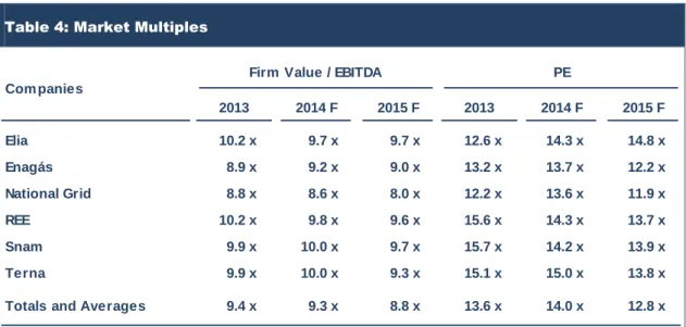
Market Multiples
3.1. Market Multiples’ Families
When market multiples are inferred based on peer companies’ quotes it is usual to designate this approach as market comparable. When the evaluation referential used to determine these multiples
corresponds to the prices paid in M&A operations, this approach is usually designated as transaction comparable.
Figure 2: Market Multiples’ Families
Source: Author elaboration.
The value referential determined with basis on the transaction comparable method tends to be superior to the ones calculated with basis on the companies’ quotes, since the prices paid in M&A operations normally embody significant premiums compared to the current prices:
Chart 8: Average Premium Paid in M&A18 Operations
Source: McKinsey (April 2013).
http://www.mckinsey.com/insights/corporate_finance/m_and_a_in_2012_picking_up_the_pace.
Apart from the value referential used to determine the market multiples, these ratios can be calculated based on the companies’ values or in the values of their equity capital.
In the first case, the multiple denominators should correspond to the economical measure that constitutes proxies of the companies’ free cash flows. In the second case, the denominators of the ratios should constitute proxies of their equity cash flows.
18
Weekly premiums = Announced price / quote one week prior to transaction announcement date.
Multiples Families
Market Comparable
Enterprise Value
Multiples Equity Value Multiples
Transaction Comparable
Enterprise Value
Multiples Equity Value Multiples
23 31 32 28 19 25 23 23 19 18 30 29 30 31 32 1998 1999 2000 2001 2002 2003 2004 2005 2006 2007 2008 2009 2010 2011 2012
3.2. Enterprise Value Multiples
The best possible proxy of the companies’ value would naturally consist in the structuring of multiples whose denominators corresponded to the normalized free cash flows of peer companies.
Unfortunately, in most cases, there is no available information that enables to determine peer companies’ normalized free cash flows. Hence, this multiple is not generally applied.
Regarding the components used to calculate free cash flows and considering that, in the long term, the variation of the companies’ working capital does not tend to be expressive and the costs with amortizations are approximately equivalent to the expenditures with investment, a second reasonable proxy of the free cash flows corresponds to the NOPLAT.
Nevertheless, market analysts do not tend to present values for this measure, reason why it is hard to reach a consensus.
Most market analysts present, nonetheless, estimates for the companies’ operational (EBIT) results. This way, and assuming that tax rates to which companies are subject do not differ significantly, the multiple which is most widely used to determine the companies’ value is the result of the division between the peer companies’ firm value and the consensus estimates of its operational results (MEBIT).
EBIT V M L
EBIT (31)
This multiple can, however, be influenced by the accounting practices adopted by the companies in what concerns the amortization basis. And, because of that, many investors prefer to utilize the multiple that compares the companies’ market value with its operational cash flows (MEBITDA):
EBITDA V
MEBITDA L (32)
However, this last multiple, contrary to what happens in those with EBIT as the denominator, does not clearly reflect the intensity of the companies’ capital: two companies from the same sector of activity can present extremely different levels of capital intensity if, for example, one has its own facilities and the other opts for renting facilities.
There are, still, other multiples that can be estimated to develop this evaluation methodology, such as the ones which compare the values of peer companies based on their respective sales, accounting value of the invested capital or productive capacities and, sometimes, their client number. However, these multiples do not reflect the return levels of companies, and therefore their relative quality is clearly inferior to the previously mentioned ones.
In the specific case of companies subject to economic regulations it is usual to resort to market-to-asset ratios (MAR) which compare these companies assets’ market value (firm value) with the book value of their regulated asset base (RAB).
3.3. Equity Value Multiples
Equity multiples are calculated with basis on ratios which have as numerator the value of the peer companies’ equity capital and as denominator those companies’ equity cash flows’ proxies, namely their dividends, net income, net cash flows or equity book value.
As the measures that can be used as denominators of these multiples can be influenced by the companies’ accounting practices and/or by its capital structure, the relative quality of these multiples tends to be inferior to that of the companies’ value multiples.
4.
Development of Multiples Valuation
The development of a valuation based on market multiples requires:
1. The structuring of a sample of companies which develop their activity in the same sector as the one object of the valuation;
2. The identification of possible factors which differentiate peer companies from the one to be evaluated, as, for example: (i) accounting rules; (ii) return and risk exposure levels; or (iii) levels of capital’s intensity;
3. Processing of all collected information on peer companies so as to make it compatible with the information on the company to be evaluated;
5. The application of determined multiples to the relevant economic variables of the company which will be subject to valuation.
Anyway, a company’s evaluation using the method of the market comparable is not a particularly rigorous or reliable exercise.
Firstly, because, for the reasons already mentioned, it is not easy to identify companies that meet the necessary conditions that enable to classify them as a peer company of the one which will be subject to valuation. And, secondly, because multiples only serve as proxies of a relation between the companies’ value or its equity capital with the variable which determines those value referential: the estimated future income series.
In this context, investors do not tend to elect the comparable method as the main valuation methodology when making their investment decisions, namely when these decisions are relevant, basically only using it to assess the conclusions obtained with the application of more reliable evaluation methods, such as the income method.
IV.
Other Valuation Methods
1.
Patrimonial Method
The use of the patrimonial method requires the conversion of the accounting balances of the companies’ assets and liabilities into their respective market values, the main differences between these two value metric criteria normally being in terms of medium and long-term assets and liabilities.
This valuation method does not tend to be particularly used by investors when intending to assess the value of a company considering the optical continuity of operations (going concern), since the patrimony historically accumulated by the companies does not tend to be representative of its capacity to generate future income.
In these circumstances, the patrimonial value method tends to be used in the determination of the net value of companies.
2.
Real Options Method
Finally, there is the contingent claim valuation, also known as option theory, which is used to value flexibility. This method is especially significant when valuing individual businesses or projects.
The option theory is not frequently used when valuing the whole company, but it can be used in very concrete cases such as firms in a commodity-based industry, firms with a single product or firms facing financial distress (Koller et al. 2005).
Regarding the real option valuation, the Black and Scholes model (1972) can be applied, because managers can easily convert the financial variables into the project’s characteristics.
Hereupon, this approach is majorly used when it is necessary to decide whether to explore or not an opportunity (Luehrman 1997), i.e., in deciding if it is beneficial to exploit natural resources, R&D investments and new technology projects. In these cases, this methodology is more appropriate, since traditional DCF will lead to results of under or overinvestment.
Given that the fundamentals of this method do not fit with those of REN, the option theory will not be applied.
V.
REN Group Valuation Methods and Parameters
1.
Valuation Methods
Taking into account the characteristics of the different valuation methods and REN Group‘s profile (briefly described in the following chapter), it was decided to use the discounted free cash flows method (based on the present value or adjusted rate of return) and market multiples to proceed to the estimation of the value of the Group.
To determine the final value to be assigned to REN Group’s shares the recent evolution of the respective quotes and price targets which market analysts assign them have also been taken into account.
2.
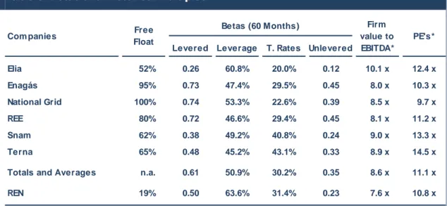
Sample of Peer Companies
The sample of selected peer companies includes:(i) Elia; (ii) Enagás; (iii) National Grid; (iv) REE; (v) Snam; and (vi) Terna.