Improving public health in smart cities in the air pollution context

(1)

i

Improving public health in smart cities in the air pollution

context

(2)

ii

IMPROVING PUBLIC HEALTH IN SMART CITIES IN THE AIR POLLUTION CONTEXT

Dissertation supervised by

Prof. Ramos Francisco, Universitat Jaume I, Castellón, Spain co-supervised by

Prof. Cristina Costa, Universidade Nova de Lisboa, Portugal Prof. Judith Verstegen, University of Münster, Germany

(3)

iii

Acknowledgements

I thank the Almighty God for the gifts of life, prayer, protection and continued guidance in my life that has always been my source of encouragement to take the next step in life.

I thank all my supervisors Prof. Ramos Francisco, Prof. Cristina Costa and Prof. Judith Verstegen for their continued guidance that gave me renewed energies at every step throughout the master thesis. Special thanks go to Prof. Ramos Francisco, Dr Sergi Trilles Oliver whom I worked closely with from the start of the master thesis till the end and Andres Munoz during the routing service implementation.

I thank my family members and friends whose continued love, support, encouragement and confidence in me has increased my efforts in becoming a better person both in my career and in my personal life.

I thank all my professors during this master program for helping me acquire knowledge and skills that will help me take the next step in my career in offering better and advanced solutions in diverse fields.

(4)

iv

IMPROVING PUBLIC HEALTH IN SMART CITIES IN THE AIR POLLUTION CONTEXT

Abstract

The public has continually developed interest in knowing the air quality around them. This is of great importance not only for planning their activities, but also for taking precautionary measures for their health. With support from smart cities infrastructure that supports taking measurements of pollutant concentrations, several countries and researchers have used the concept of air quality index (AQI) in its different forms of air quality or air pollution to interpret and communicate such measurements.

In this study we have reviewed the implemented indices by government bodies and some formulations from researchers in relation to the available data to determine an optimum index for Madrid city. This comparison has helped to formulate the Madrid Local Air Quality Index (MLAQI), which considers the local situation in Madrid city.

In relation to the available data from the city council, we have reviewed and compared some of the spatial interpolation methods that have been applied in the field of air pollution. This helped us to identify IDW for support of automated hourly pollution interpolation for the available data from Madrid pollution sensors.

We have then used MLAQI and IDW to create an hourly pollution Web Feature service aimed at helping with public awareness of the air quality around them. The surfaces are categorised with the index categories from good to very poor categories with defined colour coding.

We used the created service to develop a routing web application where high MLAQI categories of poor and very poor are used as polygon barriers to limit the route calculation in those polluted areas thereby helping the public to protect their health from such areas.

(5)

v

Key words

Public health Air Quality Index Air Pollution Index Pollutant concentrations Spatial interpolation Web feature service

(6)

vi

Acronyms

AQI – Air Quality Index PSI – Pollution Quality Index

MLAQI – Madrid Local Air Quality Index CO – Carbon Monoxide

SO2 – Sulfur Dioxide O3 – Ozone

PM10 – Particulate Matter 10 micrometers or less in diameter PM2.5 – Particulate Matter 2.5 micrometers or less in diameter NO2 – Nitrogen Dioxide

WFS – Web Feature Service

REST – Representational State Transfer JSON – JavaScript Object Notation

ESRI – Environmental Systems Research Institute URL – Uniform Resource Locator

(7)

vii

Index of tables

Table 1: Summary of reviewed indices from government bodies and the research community .. 11

Table 2: Summary of the used spatial interpolation methods in air pollution ... 14

Table 3: Comparison of air quality indices and the available data ... 20

Table 4: Madrid Local Air Quality Index ... 23

Table 5: Summary statistics of Exploratory Spatial Data Analysis ... 34

Table 6: An extract of model parameters and their errors with IDW structural modelling ... 35

Table 7: Error summary from variogram using same model parameters ... 35

(11)

xi

Index of figures

Figure 1: Sensor stations location and types ... 19

Figure 2: Madrid sensor stations combination scenarios ... 22

Figure 3: The spatial distribution of sensor stations with MLAQI ... 24

Figure 4: Implementation workflow ... 25

Figure 5: Categorised IDW interpolation output according to MLAQI ... 37

Figure 6: A screenshot of the developed application ... 38

(12)

1

1 Introduction

1.1 Background to the study

Smart cities use information technologies to improve on the performance and quality of urban services, to decrease costs and optimize resources, and more so they involve citizens to participate actively in such activities(Zanella et al., 2014). Among the various areas developed in such a context, this study focuses on public health. There has been increasing public need for better air quality or for avoidance of air pollution, which has led to the establishment of determination and representation approaches of these occurrences continuously using the index concept in their formulations.

In recent years, air pollution control has demonstrated to have a positive impact on public health (Correia et al., 2013). A control measure taken by governments or local administrations involves using specific sensors distributed over a wide area usually named air pollution sensors, which are able to detect different levels of air pollution in a particular location.

Deployment of these sensors is slightly growing up with Smart cities and Internet Of Things(Zanella

et al., 2014), which enables us to obtain access to their produced data. However, the information

usually provided to the users is one-dimensional based, in this case corresponding to a determined and fixed latitude and longitude where the sensor is installed.

Many works have been done to publish or generate two-dimensional data from those types of sensors, among these we underline the ones using interpolation methods that use spatial analysis applying statistical theory and techniques to model spatially referenced data.

In our context, pollutant concentrations are types of data that can be represented by surfaces where each raster cell represents a measurement such as a cell’s relationship to a fixed point or specific concentration level. Due to impracticability of obtaining values for each cell in a raster, sample points are used to derive the intervening values using interpolation methods. This ability to create surfaces from sample data of air pollution sensors makes spatial interpolation both powerful and useful for the study.

In disseminating pollution information, several government bodies and industry players publish pollutant concentration levels on their websites or mobile applications. The published information can be in the form of pollutant concentrations or scaled concentrations based on a particular air quality or air pollution index. Some of these indices provide health related recommendations to the general public or specific groups of people for the different levels of pollutant concentrations.

(13)

2

1.2 The study area

The chosen study area is Madrid city, the capital of Spain. The city has had challenges with air pollution and has continuously set up measures to control this pollution challenge. One of the measures used for management and control of this challenge is the use of a network of automatic monitoring stations and other mobile stations for measuring pollutant concentrations and calibration of the measurement equipment.

In engaging the public on the awareness of the air quality around them, the city council implemented an air quality information system which disseminates such information to the public in various ways like sms, emails, website, “Aire de Madrid” mobile application and public displays. The hourly pollutant concentration levels are communicated to the public through the hourly index while the daily levels are communicated through the daily index. The daily communication includes maps of the air quality prediction surfaces for a particular day and the following day are categorised by zone in Madrid. The city council also publishes pollutant concentration values through the open data portal for researchers and application developers to use in studies about this challenge in the city.

1.3 Problem statement

The public has continuously developed interest in knowing the state of the air quality, which has supported the development of various approaches for air pollution concentration measurements, representation and dissemination of the resulting information to the public.

As the Madrid city council offers the necessary infrastructure and information services to take pollution concentration measurements, this has enabled reporting about the state of air quality in the city to the public. The reports are mainly the pollutant concentrations at the locations of sensor stations scaled on a given index with a colour representation and the daily prediction pollution surfaces together with a prediction surface for the following day categorised by the different zones of Madrid.

With the city’s pollutant concentration values becoming too high at certain hours, daily pollutant prediction surfaces categorised by zones may not effectively help the public to plan their hourly activities or avoid certain areas with high pollutant concentration values at certain hours. This presents a need for an hourly pollution surface service which service can be used by the general public in planning their hourly activities or be incorporated in other services of public interest like routing for the public to use in their navigation between locations of interest.

(14)

3

1.4 Aim

To develop an hourly air pollution surface service for Madrid city that will help the public to be aware of the air quality around them and be in position to make informed decisions while planning their activities around the city.

1.5 Objectives

In achieving the study’s aim, we will meet several objectives.

 Review and analysis of existing index approaches used in communicating air quality or air pollution.

 Review and analysis of different interpolation techniques, both deterministic and geostatistical ones used in the field of air pollution.

 Modification of the existing Madrid Air Quality Index for better air pollution representation with support of spatial interpolation.

 Obtaining and aggregating the Madrid city council open portal published pollution data to support index calculation using the modified index.

 Perform spatial interpolation on the computed index and creating hourly raster surfaces for the index.

 To support the dissemination of these results to smart citizens and improve their health, there is a need for creating a real-time conversion service to generate vector geometries from the interpolated raster surfaces into categories of Good, Acceptable, Poor and Very Poor according to the index.

 To facilitate the data access and exploitation from final applications, we had to create an automatic hourly publishing service for publishing and sharing the created vector surfaces online.

 Implementing a web application using the published service to help the public plan a path to walk or run by minimizing the high pollution areas to traverse, a way to improve their health.

1.6 Hypothesis

Air pollution concentration measurements from a Smart city’s infrastructure can support the generation of hourly pollution surfaces, which can help protect the health of citizens. These surfaces can be incorporated into activities of public interest to help the public make informed decisions about such activities.

(15)

4

1.7 Limitations

The study is limited to the available published data from active sensor stations in Madrid city. The number of stations may affect the accuracy of spatial interpolation.

The access of the ESRI routing and traffic premium services is limited to use with a proxy web server. The proxy setup requires an active ESRI developer account for generating required tokens and application registration access information. This routing service also limits the number of intersected street with polygon barriers in routing.

(16)

5

2 Literature review

2.1 Comparative study of Air Quality Indices

In pursuit of addressing air pollution issues around the globe, several approaches for reporting the studies and the results have been developed and tested. One of the approaches developed is the approach of air quality index that seeks to represent the level of the air quality in a location of interest. The indices developed consider different pollutants and use varying limits in reporting the results.

The study compares some of the formulated indices from governmental bodies and the research community, some of which several government bodies have implemented. To compare these approaches, the study is based on their definitions and calculation, categories considered with the category ranges, the symbology used in their representations, the general health recommendations to the public and to specific groups of people, the effect of multi-pollutants and concentration measurement location variations.

2.1.1 The United States Environmental Protection Agency (EPA) Air Quality Index (AQI)

The US EPA AQI categorises air quality in six categories of Good with range (0-50), Moderate with range (51-100), Unhealthy for Sensitive Groups with range (101-150), Unhealthy with range (151-200), Very Unhealthy with range (201-300) and hazardous with range (301-500). With this AQI, the values above 500 are also considered hazardous (US EPA, 2014). These categories increase with increasing effect on human health and are assigned standard colours for easier identification and reporting (US EPA, 2013).

This AQI is defined for pollutants of Ozone, PM2.5, PM10, Carbon monoxide, Nitrogen Dioxide and Sulfur Dioxide. These pollutants (O3, PM1, PM2.5, PM10, CO, NO2, and SO2) are also critical for research and Industrial IoT system deployment with US EPA-funded testing facilities like AQ-SPEC at the Southern California Air Quality Management District (SC - AQMD) in Los Angeles, California (Valarm, 2018). The EPA also defines the limit values for specific time scales of these pollutants for computation of the AQI. For Ozone, the limit values are defined for 1hour and 8hours, for PM 2.5 and PM10, the limit values are defined for 24hours, for Carbon monoxide, the limit values are defined for 8hours and the limits for Nitrogen Dioxide and Sulfur Dioxide are defined for 1hour. Higher values of limit values do not indicate higher AQI but are the basis for calculation of the index (US EPA, 2013). At the established categories, the AQI defines health related risks or groups of people that are highly affected by the levels of air pollution.

(17)

6

2.1.2 The Canada Air Quality Health Index.

The Canadian government uses an Air Quality Health Index (AQHI) developed based on the relative risk of pollutants to human health with a scale designed to help people understand what the air quality around them means to their health. It helps people make decisions regarding short-term exposure to air pollution and adjusting their activities based on the information obtained (Stieb et

al., 2008; ECCC Canada, 2016).

The AQHI communicates the air quality health related risks on a scale of 1 to 10+ with 4 categories of health risks as Low Health Risk (1-3), Moderate Health Risk (4-6), High Health Risk (7-10), or Very High Health Risk (10+). A colour scheme of light blue for lower values of the index to brown for higher values of the index is used in the index communication. It also gives the health messages for both the population at risk and the general population. AQHI uses the relative risks of a combination of pollutants of Ozone, PM2.5 and Nitrogen Dioxide to determine the final index.

2.1.3 Common Air Quality Index (CAQI)

Developed under the CITEAIR project of the European Union with the aim of establishing a platform for comparing air quality across the different cities in Europe, a review of the existing indices was carried out and CAQI developed to achieve the comparability across the cities in real-time and caters for hourly, daily and yearly real-time scales. It established two indices, one for the roadside monitoring stations and the other one for city background conditions (van den Elshout, Léger and Nussio, 2008). CAQI defines five classes with appropriate ranges of Very Low (0-25), Low (25-50), Medium (50-75), High (75-100) and Very High (above 100).

The first version of CAQI considered pollutants of Ozone (O3), PM10, Carbon monoxide (CO), Nitrogen Dioxide (NO2) and Sulfur Dioxide (SO2) but the revised version of the index introduced PM2.5 in the index calculation (van den Elshout, Léger and Nussio, 2008; Van Den Elshout, Léger and Heich, 2014). CAQI uses the concept of core pollutants for the two indices, introduced to allow for the calculation of the index and without it an index calculation is not performed. For the roadside index, the core pollutants considered are NO2 and PM10 with CO and PM2.5 as auxiliary pollutants while for the city background index NO2, PM10 and O3 are considered core pollutants with CO, SO2 and PM2.5 considered as auxiliary pollutants. The index is calculated by linear interpolation between the class borders ofthe pollutants and the final index given as the highest sub index of the considered pollutants (van den Elshout, Léger and Nussio, 2008; Plaia and Ruggieri, 2011).

(18)

7

2.1.4 The UK Air Quality Index

In a review of the UK Air Quality Index, Committee on the Medical Effects of Air Pollutants (COMEAP) developed and recommended a Daily Air Quality Index (DAQI) for the purpose of providing short-term health advise to the public regarding the air quality around them and possible recommendations such people can take (COMEAP UK, 2011). Following the recommendations from COMEAP, the Department for Environment, Food and Rural Affairs (Defra) together with responsible administrations implemented this index from January 2012. This Index was later updated with minor changes through Defra’s update on the implementation of DAQI in April 2013 to conform with the EU limit values of pollutant concentrations. The update also emphasised that data rounding off should always be performed at the end of calculations before communicating results to avoid errors (Emily Connolly et al., 2013).

DAQI is defined on a scale of 1 to 10 with colour coding and categorised into four bands of Low (1-3), Moderate (4-6), High (7-9) and Very High (10) (COMEAP UK, 2011). COMEAP report recommended the removal of CO from the AQI and the inclusion of PM2.5. Currently the DAQI uses the pollutants of Ozone (O3), Nitrogen Dioxide (NO2), Sulfur Dioxide (SO2), PM2.5 and PM10 in calculation of the index. The Automatic Urban and Rural Network (AURN) measures these pollutant concentrations in near real-time and their values used in calculation of the index (COMEAP UK, 2011). The overall index is given by the highest pollutant concentration of the considered pollutants. To allow prediction of elevated air pollution episodes in real-time, DAQI uses trigger values to predict concentrations of pollutants (COMEAP UK, 2011).

2.1.5 Ireland Air Quality Index

In order to find an appropriate Air Quality Index for Ireland that included health information, Air Quality Health Information Working Group was set up in 2011 for the task. The Health Service Executive (HSE) reviewed existing health based evidence on the impact of air pollution on health and also reviewed a selection of Air Quality Indices that existed across the globe. The committee reached similar conclusions to those done by the COMEAP. This led to the proposal by the Irish Environmental Protection Agency (EPA) for adopting the UK DAQI into the Irish air quality monitoring infrastructure. The HSE and Irish EPA reached the conclusion of introducing the Air Quality Index for Health (AQIH) that is closely aligned with the UK DAQI.

The AQIH was proposed to maintain consistency with the previous Irish index that was also an air quality index. It is noted that the UK DAQI is a pollution index as it was replacing a previous air pollution index. This difference led to the difference in the naming of the index categories (EPA

(19)

8 Ireland, 2013a). The Irish AQIH uses a scale with defined colour coding of 1 to 10 that is categorised into four bands of Good (1-3), Fair (4-6), Poor (7-9) and very poor (10) (EPA Ireland, 2013b). These bands correspond to the UK DAQI bands of Low, Moderate, High and Very High respectively. The other information like health messages and interpretation of the index is the same. Like the DAQI, AQIH considers five pollutants of ozone, nitrogen dioxide, sulphur dioxide, PM2.5 and PM10. The final index is given by the worst index of the separately calculated indices of the considered pollutant concentrations.

2.1.6 Spain, Madrid Air Quality Index

Madrid City Council provides information to its community using an air quality index defined by a scale of 0 to >150 with four categories of “Buena” - good (0-50), “Admisible” - acceptable (51-100), “Deficiente” - poor (101-150) and “Mala” - very poor (>150). The City council uses the pollutants of PM10, Sulfur Dioxide, Nitrogen Dioxide, Carbon Monoxide and Ozone. Sub indices are calculated for the considered pollutants and the final index is the worst sub index of the pollutant concentrations (Madrid City Council, 2015).

2.1.7 France Air Quality Index

The ATMO Index is the air quality index used in major cities in France that have a population of more than 100,000 inhabitants. The index is represented by a giraffe and is based on a scale of 1 to 10 ranging from very good to very bad and with three coloured bands of Green (1-4), Orange (5-7) and Red (8-10). ATMO Index considers the pollutants of Sulfur Dioxide, Nitrogen Dioxide, Ozone, PM2.5 and PM10. Sub indices are calculated for the four pollutant concentrations and the final aggregated index is the highest sub index calculated from the pollutant concentrations (ATMO France, 2008). Each pollutant has defined limit values for the scale ranges upon which pollutant concentrations are compared to determine the pollutant sub index.

2.1.8 Singapore Air Quality Index

Singapore reports air quality in terms of Pollutant Standards Index (PSI). The index is categorised into five categories of Good (0-50), Moderate (51-100), Unhealthy (101-200), Very Unhealthy (201-300) and Hazardous (301-500) (NEA Singapore, 2017). PSI is based on six pollutants of PM2.5, PM10, Sulfur Dioxide, Carbon Monoxide, Ozone and Nitrogen Dioxide. The sub indices of all the considered pollutants are calculated and the final index is the highest sub index of the pollutant concentrations (NEA Singapore, 2014).

(20)

9

2.1.9 Researchers work on Air Quality Index representation

Several researchers have continued to investigate on the better representation of air quality index. We have specifically selected five published papers detailing some of these methods which are related with health, the effect of multi pollutants on heath and spatial variability of pollutant measurement locations.

To account for multi pollutant short-term health effects of exposures on the final index, (Cairncross, John and Zunckel, 2007) formulated an Air Pollution Index (API). To account for this effect, the final index is the summation of the normalised sub indices of pollutant concentrations. The developed index depends on the relative risk of daily mortality associated with the common pollutants of PM2.5, PM10, Sulfur Dioxide, Nitrogen Dioxide, Ozone and Carbon Monoxide. The proposed index has a scale of 1 to 10 with defined colour codes. It also defines the index with four categories together with associated increase in mortality risks. The four categories are low (1-3), moderate (4-6), high (7-9) and very high (10).

Based on time series analysis of air pollution and mortality in Canadian cities, (Stieb et al., 2008) proposed an Air Quality Health Index (AQHI). To cater for multi pollutant effects and varying seasons, they carried out analysis for pollutant combinations using single and multi pollutant models and for varying seasons. To develop the index, they used the combination of Carbon Monoxide, Nitrogen Dioxide, Ozone, PM2.5 or PM10 and Sulfur Dioxide pollutants. The index excludes Sulfur Dioxide and Carbon Monoxide in its formulation after realising their small effect during the analysis. The index is defined by four different scenarios using PM2.5, PM10, warm and cool seasons for the case of PM2.5. The index created is on a scale of 0 to 10+ with categories of Low risk (0-3), Moderate risk (4-6), High risk (7-10) and Very high risk (above 10). A corresponding colour scheme is also defined along the scale with colours ranging from light blue at low AQHI values to brown at high AQHI values and red for very high risk category. It provides health related messages to the population at risk and the general population.

Using the pollutants of Carbon Monoxide, Sulfur Dioxide, Nitrogen Dioxide, Ozone and PM10, (Kyrkilis, Chaloulakou and Kassomenos, 2007) developed the aggregate Air Quality Index for Athens, Greece. To cater for multi pollutant effects, they adopted an aggregate function to compute the overall index of the city. They compared their results with the modified USEPA AQI using the European pollutant standard limits and found the modified USEPA predicted higher values than the developed aggregate AQI.

(21)

10 In studying multi-pollutant effects and relative risks of short-term exposure to pollutants, (Sicard

et al., 2011) developed the Aggregate Risk Index. The ARI is based on the exposure response

relationship and relative risk of established effects to assess the additive effects of pollutants. The method used published relative risk functions data and particular sets of relative risks for associated health risk end points to derive the index. The ARI considers the relative risks of Sulfur Dioxide, Nitrogen Dioxide, PM2.5, PM10 and Ozone pollutants. In catering for the multi pollutant effects, the final index is the summation of individual calculated risk indices. The index is defined from 0 to 10 with the risk values used to derive the break points. The index is categorised into Low (1-3), Moderate (4-6), High (7-9) and Very high (10) with appropriate information about the excess relative risk of mortality or morbidity.

In considering the additive effects resulting from multi pollutants and the effect of measuring pollutants over different geographical locations, (Murena, 2004) developed a daily Air Pollution Index (PI) modified out of the US EPA AQI. The developed index uses European limit values in its computation. The index uses the common pollutants of Carbon Monoxide, Nitrogen Dioxide, PM10, Sulphur Dioxide and Ozone in its computation. The index is defined on a scale of 0 to 100 and it defines five categories of Good quality (25), Low pollution (50), Moderate pollution (70), Unhealthy for sensitive groups (85) and Unhealthy (100). The index introduced clouds for representing the pollution categories. The method introduced considers the sum of ratios of daily reference concentrations of pollutants and their bottom breakpoint concentration values to cater for multi pollutant additive effects on human health and introduces weights for geographical location variability of sensor measured pollutants concentrations.

2.1.10 Summary of the reviewed indices

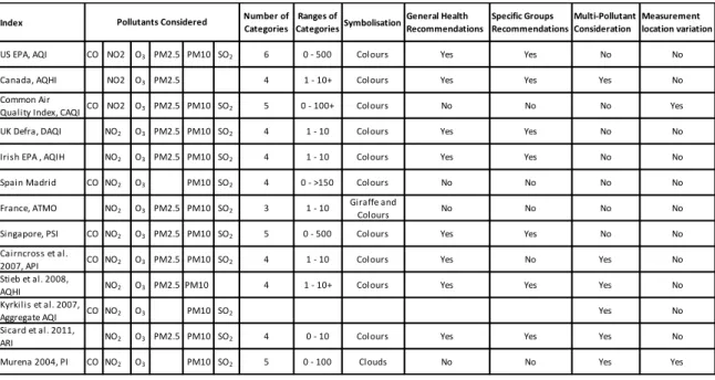
The reviewed indices share and differ in some of their formulations and representations Table 1. To relate these indices, we have summarised them in terms pollutants considered in their formulation, the number of categories and ranges they consider, the symbolisation and graphical representation used, the health recommendations for the categories, the effect of multi pollutants and the spatial variability of concentration measurement locations.

(22)

11

Table 1: Summary of reviewed indices from government bodies and the research community

From Table 1, most indices share pollutant compositions with Ozone and Nitrogen Dioxide pollutants being common to all. They vary in the formulation of categories ranging from 3 to 6 with the mode number of categories being 4. Apart from two indices one of which colour symbology is undefined and the other one using only clouds, all other indices use colour symbology spread over their respective categories. Most indices give general and specific health recommendations to the public. The indices from the research community considered more the effect of multi-pollutants compared with the researched or implemented indices by government bodies. Most indices do not consider the location variability of pollutant measurements.

2.2 Spatial interpolation methods in air pollution

2.2.1 Spatial Interpolation

Spatial interpolation involves estimation of values of a desired attribute of a phenomenon at unsampled points using the values of sampled points in the estimation or prediction process. Miller associated Tobler’s first law of geography as being core to spatial auto correlation, spatial interpolation and techniques for predicting missing variables in a geographic space (Miller, 2004). Tobler’s first law of geography states that: “everything is related to everything else, but near things are more related than distant things” (Tobler, 1970). In situations that involve continuous variables like elevation of the landscape, pollutant concentrations in the atmosphere and temperature, it is challenging to take measurements at every location to represent such phenomena, thus the power of spatial interpolation that facilitates the prediction of intermediate values from sampled locations and makes it possible to represent such phenomena as surfaces. Spatial interpolation is

Index Number of _Categories _CategoriesRanges of SymbolisationGeneral Health _{Recommendations} Specific Groups _{Recommendations}Multi-Pollutant _{Consideration} Measurement _{location variation}

US EPA, AQI CO NO2 O3 PM2.5 PM10 SO2 6 0 - 500 Colours Yes Yes No No

Canada, AQHI NO2 O3 PM2.5 4 1 - 10+ Colours Yes Yes Yes No

Common Air

Quality Index, CAQI CO NO2 O3 PM2.5 PM10 SO2 5 0 - 100+ Colours No No No Yes UK Defra, DAQI NO2 O3 PM2.5 PM10 SO2 4 1 - 10 Colours Yes Yes No No

Irish EPA , AQIH NO2 O3 PM2.5 PM10 SO2 4 1 - 10 Colours Yes Yes No No

Spain Madrid CO NO2 O3 PM10 SO2 4 0 - >150 Colours No No No No

France, ATMO NO2 O3 PM2.5 PM10 SO2 3 1 - 10 Giraffe and

Colours No No No No

Singapore, PSI CO NO2 O3 PM2.5 PM10 SO2 5 0 - 500 Colours Yes Yes No No

Cairncross et al.

2007, API CO NO2 O3 PM2.5 PM10 SO2 4 1 - 10 Colours Yes No Yes No

Stieb et al. 2008,

AQHI NO2 O3 PM2.5 PM10 4 1 - 10+ Colours Yes Yes Yes No

Kyrkilis et al. 2007,

Aggregate AQI CO NO2 O3 PM10 SO2 Yes No

Sicard et al. 2011,

ARI NO2 O3 PM2.5 PM10 SO2 4 0 - 10 Colours Yes Yes Yes No

Murena 2004, PI CO NO2 O3 PM10 SO2 5 0 - 100 Clouds No No Yes Yes

(23)

12 very useful in many fields like environmental modelling, surveying, mining, civil engineering, agriculture, etc., that involve the need of representing several phenomena as surfaces.

Spatial interpolation is classified into three categories of non-geostatistical, geostatistical and methods that combine both geostatistical and non-geostatistical techniques (Li and Heap, 2008). Features that distinguish and offer comparison of these spatial interpolation methods are discussed in (Li and Heap, 2014). These features include: The global and local nature of prediction where the global predictors use the entire sample points in the prediction process while the local use part of the points near the un known point for its prediction, the exactness of the interpolator where the exact interpolators resulting in a prediction that is the same as the observed value at the sampled location while the inexact results in a value that is different from the value at the sampled location, the deterministic and stochastic nature of the prediction.

2.2.2 Deterministic and stochastic spatial interpolation methods

The deterministic interpolators produce predictions without assessing the errors in the prediction process. The deterministic methods include Nearest neighbour (NN), Triangulated irregular network (TIN), Natural neighbour (NaN), Inverse distance weighting (IDW) and Radio Basis Functions (RBF) (Li and Heap, 2008; Adhikary and Dash, 2017). Stochastic interpolators produce predictions in both the deterministic part and provide the error assessment part. These include Regression models (LM) and Kriging (Li and Heap, 2008). Several researchers have used both deterministic and stochastic methods to represent different phenomena in terms of surfaces. Some studies have also compared the performance of different methods in representing different phenomena (Anselin and Le Gallo, 2006; Rojas-Avellaneda, 2007; Pultar et al., 2010; Kumar Jha et

al., 2011; Singh et al., 2011; Joseph et al., 2013; Adhikary and Dash, 2017).

2.2.3 Spatial interpolation studies with air pollution

In building an environmental quality index for Madrid city, Spain, (Montero, Chasco and Larraz, 2010) used Ordinary Kriging to produce surfaces of SO2, CO, NOx, NO2, PM, O3 and noise from monitoring stations in Madrid city and linked this data with census tracts data. In their study, they reported variation of precision for locations that were further away from the monitoring stations. They used 27 monitoring stations for the annual averages of daily readings for the year 2001 for their study.

In modelling NO2 and PM10 in the metropolitan areas of Barcelona and Bilbao, Spain, (Lertxundi-manterola and Saez, 2009) used Ordinary kriging to interpolate the daily averages of NO2 and PM10 across the cities. They obtained a disappearing spatial dependence of concentrations at a

(24)

13 distance of 1-3km from the monitoring stations. For the case of Barcelona, they used 9 monitoring stations for both pollutants and for the case of Bilbao, they used 28 monitoring stations for NO2 and 10 for PM10.

In analysing the sensitivity of hedonic models of price houses with interpolation of air quality measures in Southern California, USA, (Anselin and Le Gallo, 2006) needed to assign O3 levels to house transaction locations. They tested four interpolation methods of Thiessen polygons, IDW, Ordinary kriging and spline and found Ordinary kriging offering consistent fit and reasonable parameters for their study. They used O3 measurements from 27 monitoring stations.

In analysing environmental justice of particulate air pollution in Hamilto, Canada, (Jerrett et al., 2001) used Universal kriging to create pollution surfaces from pollutant concentration data of 23 monitoring stations and linked the results with the social economic and demographic data of Hamilton. They based on prior knowledge of existence of a spatial trend in the particulate data of Hamilton to choose universal kriging against ordinary kriging.

In predicting the pollutant concentrations in Mexico City, Mexico using interpolation methods, (Rojas-Avellaneda, 2007) identified IDW and kriging as the most used spatial interpolation methods in pollutant concentration prediction. The study compared IDW and Simple kriging methods using O3 concentration measurements from 20 monitoring stations at a specific time for 21 days. Both methods performed better with a consideration of a linear drift in the data and produced closely related results.

In mapping the background air pollution across Europe, (Beelen et al., 2009) compared the performance of three modelling techniques of Universal kriging, Ordinary kriging and a regression model. They considered pollutants of NO2, O3, PM10, SO2 and CO using the Airbase data and the predictor variables used were from EU-wide databases. The results for NO2, O3 and PM10 showed better performance of Universal kriging compared with the other two methods while none of the methods predicted SO2 and CO satisfactorily.

In assessing spatial interpolation methods for O3 exposure predictions, (Joseph et al., 2013) used data from two urban areas of Los Angeles, California USA, with 27 monitoring stations and Houston, Texas, with 42 monitoring stations for the compare Simple average, Nearest neighbour, IDW, Ordinary kriging and Universal kriging. The results indicated the superiority of Ordinary kriging with a calibrated range parameter in comparison with the other tested methods.

In mapping hourly O3 episodes for spring and summer periods in Eastern Texas, USA, (Kethireddy et al., 2014) used Ordinary kriging to interpolate and map O3 at a 1km spatial scale with 80

(25)

14 monitoring stations. The study detected episodes of O3 during afternoon hours and found Ordinary kriging to successful predictions of this pollutant in the study area.

2.2.4 Summary of the used spatial interpolation methods in air pollution

Table 2 shows the summary of the reviewed studies in relation to spatial interpolation and air pollution. These have been summarised with the pollutants considered and the number of used monitoring stations.

Study Methods Best method from

comparison studies

Pollutants considered

Number of sensors (Montero, Chasco and

Larraz, 2010)

Ordinary Kriging SO2, CO, NOx, NO2,

PM, O3, noise

27 (Lertxundi-manterola

and Saez, 2009)

Ordinary Kriging NO2, PM10 9, 28, 10

(Anselin and Le Gallo, 2006)

Thiessen polygons, IDW, Ordinary kriging and spline

Ordinary kriging O3 27

(Jerrett et al., 2001) Universal Kriging 23

(Rojas-Avellaneda, 2007)

IDW, Simple Kriging IDW O3 20

(Beelen et al., 2009) Universal kriging, Ordinary kriging and a regression model

Universal kriging NO2, O3, PM10,

SO2, CO

(Joseph et al., 2013) Simple average, Nearest neighbour, IDW, Ordinary kriging and Universal kriging

Ordinary kriging O3 27, 42

(Kethireddy et al.,

2014)

Ordinary kriging O3 80

Table 2: Summary of the used spatial interpolation methods in air pollution

From these studies, we found that kriging in its different forms was the widely used method of spatial interpolation in relation to air pollution and these studies also shared the similarity in the sources of used data like the data used in Madrid with one of the studies (Montero, Chasco and Larraz, 2010)conducted in Madrid. The popularity of kriging confirms earlier findings by (Jerrett

et al., 2005).

2.2.5 The general prediction equation

With most prediction methods seen as weighted data averages and using the general prediction equation (Webster and Oliver, 2007), we have used this general equation (1) to briefly describe the Inverse Distance Weighted (IDW) and Kriging methods.

𝑍̂(𝑥₀) = ∑ 𝜆_𝑖𝑍(𝑥_𝑖)

𝑛

𝑖=1

(26)

15 Where 𝑍̂ is the predicted attribute value at 𝑥₀. 𝑍(𝑥_𝑖), the data values at 𝑥𝑖… 𝑥𝑛 points. 𝜆𝑖 are the

assigned weights to the data values at those points and 𝑛 is the used number of sample points for the prediction.

2.2.6 Inverse Distance Weighted (IDW)

Also known as the Inverse Distance Weighting, IDW, is a deterministic spatial interpolation method that bases on the idea of nearer things being more related to each other than further things to assign more weights to observations near the value being predicted. IDW weights the sampled points with an inverse function of the distance from the prediction point to the sampled points. Thus from the general equation (1), IDW defines weights as given in equation (2).

𝜆_𝑖 = 1/𝑑𝑖

𝑝

∑𝑛_𝑖=11/𝑑_𝑖𝑝 (2)

Where 𝑑𝑖 represents the distance difference between 𝑥0 and 𝑥𝑖 , 𝑝 being the power parameter

and 𝑛, the number of sample points used in the prediction. Webster and Oliver noted that the power parameter choice is arbitrary (Webster and Oliver, 2007). As cited by Li and Heap, the accuracy of IDW is mainly affected by the power parameter. With 𝑝 = 0, IDW becomes moving average, with 𝑝 = 1, IDW becomes linear interpolation, with 𝑝 = 2, IDW becomes inverse square distance or inverse distance squared and when 𝑝 ≠ 1, then IDW is a weighted moving average (Li and Heap, 2008).

2.2.7 Kriging

Developed by Matheron and D.G Krige, kriging is a local, exact and stochastic spatial interpolation method. Kriging is a generic term referring to a family of geostatistical techniques that come in form of both linear or non-linear interpolators (Webster and Oliver, 2007). Kriging methods are based on the following equation (3) which is a modification from the general equation (1).

𝑍̂(𝑥₀) − 𝜇 = ∑ 𝜆_𝑖[𝑍(𝑥_𝑖) −

𝑛

𝑖=1

𝜇(𝑥₀)] (3)

𝜇, the known stationary mean is considered constant over the entire domain that is calculated as the average of the data. 𝜆_𝑖, kriging weight, 𝑛, number of sampled points for estimation within a search window and 𝜇(𝑥₀) is the mean of the sampled data within a search window.

For the purpose of this study, the focus is on the kriging methods of Ordinary kriging and Universal kriging that have been applied in similar studies more than Simple kriging.

(27)

16

2.2.8 Ordinary kriging (OK)

Within the kriging family, Ordinary kriging is the most used method (Webster and Oliver, 2007; Oliver and Webster, 2015). It assumes a randomly and spatially dependent variation whose mean is unknown and constant and the variance only dependent on the distance separation and direction between places (Oliver and Webster, 2015; Adhikary and Dash, 2017). The estimation error is expressed in equation (4)

𝜀(𝑥₀) = 𝑍̂(𝑥₀) − 𝑍(𝑥₀) = ∑ 𝜆_𝑖𝑍(𝑥_𝑖)

𝑛

𝑖=1

− 𝑍(𝑥₀) (4)

With 𝑍(𝑥0) as the true value of the variable at 𝑥0 and 𝜀(𝑥0) as the estimation error. Since the

expected residual of unbiased estimate is supposed to be 0, then

𝐸[𝜀(𝑥₀)] = 0 (5)

The weights sum to 1 to ensure an unbiased estimation resulting in equation (6).

∑ 𝜆𝑖 𝑛

𝑖=1

= 1 (6)

2.2.9 Kriging with a trend (KT)

Also known as Universal kriging, KT considers both the random and the non-stationary nature of a variable and uses both components in the estimation process. It uses the non-stationarity component to estimate the trend and uses the random component to estimate the variogram. Thus arriving at the equation (7).

𝑍̂(𝑥₀) = 𝜇(𝑥₀) + 𝜀(𝑥₀) (7)

Where 𝜇(𝑥₀) is the deterministic function which is a drift and 𝜀(𝑥0) is the random variation that

is treated to be auto-correlated. 𝑥0 represents the spatial coordinates of the data as explanatory

variables (Adhikary and Dash, 2017).

2.2.10 The variogram or semivariogram

A variogram expresses the spatial variation of an attribute and is estimated using a semi-variance of the difference between data values of the entire sampled points that are separated by a lag vector ℎ. The semivariogram 𝛾̂(ℎ) is expressed as in equation (8).

𝛾̂(ℎ) = 1

2𝑚(ℎ) ∑ [𝑍(𝑥𝑖) − 𝑍(𝑥𝑖+ ℎ)]

2 𝑚(ℎ)

(28)

17 Where 𝑚(ℎ) is the number of sample point pairs separated by ℎ. A plot of 𝛾̂(ℎ) against ℎ gives an experimental variogram with special features of nugget, sill and range.

As cited by Li and Heap, a variogram is very important in analysing the data structure (Li and Heap, 2008). The experimental variogram produced with the sampled data is fitted with variogram models like the linear, pure nugget, spherical, exponential and Gaussian models (Bayraktar and Turalioglu, 2005; Webster and Oliver, 2007, chap. 5.2; Li and Heap, 2008). The shape of the experimental variogram determines which model is applicable for a given scenario. These fitted models help in determining the variogram parameters of nugget, sill, range, the lag size, the number of lags and the neighbourhood search strategy.

Webster and Oliver noted the controversy surrounding model choice and fitting in geostatistics due variations in different determinants like semi variances, anisotropy, point to point variation in the experimental variogram and none linearity of most models in different parameters (Webster and Oliver, 2007, p. 101).

3 Methodology

To achieve the aim and objectives of the study, we have studied the available data from Madrid city council, compared it with the reviewed air quality index approaches and interpolation methods used in the field of air pollution to find an applicable index and a suitable interpolation method for the study. We have then used these approaches during the implementation phase.

3.1 Data description, comparison with reviewed AQIs and MLAQI formulation

3.1.1 The Madrid air pollution sensor network

The city council of Madrid, has a network of 24 sensor stations deployed to measure different pollutant concentrations in Madrid city to enable pollution and air quality monitoring and management. The city council of Madrid has been monitoring air quality since 1968 using a manual network and later on a set of automatic network stations since 1978. Due to the studies, developments and legislation about air quality, the city council has continued to refine and develop this network to accommodate the developments.

The sensor stations’ network continually measures the pollutants of Sulfur dioxide, Carbon monoxide, Nitrogen monoxide, Nitrogen dioxide, PM2.5, PM10, Nitrogen oxides, Ozone, Toluene, Benzene, Ethylbenzene, Metaxylene, Paraxylene, Orthoxylene, Total hydrocarbons, Methane, Non-methane hydrocarbons.

(29)

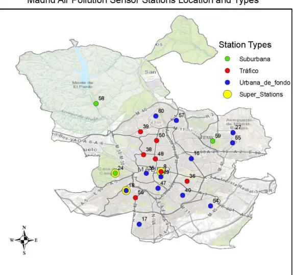
18 The stations in this sensor network are categorised into “Tráfico” - traffic, “Urbana de fondo” - Urban background and “Suburbana” - suburban. At each station several pollutants are measured but the combinations of measurements at each station are quite different. The tráfico sensor stations are mainly located along the road network and close to the city centre for detecting pollution caused by emissions on the road network while the other two types are located mainly outside the area covered by the tráfico sensor stations. The urbana de fondo sensors mainly represent the exposure of the general urban population while the suburbana are located in the city outskirts at locations of high ozone levels.

Stations are identified by station codes and pollutants identified by parameter codes for the pollutants measured at each station.

Tráfico - traffic stations. These are stations 4 (Pza. de España), 8 (Escuelas Aguirre), 11 (Avda.

Ramón y Cajal), 36 (Moratalaz), 38 (Cuatro Caminos), 39 (Barrio del Pilar), 48 (Castellana), 50 (Plaza Castilla) and 56 (Pza. Fernández Ladreda).

Urbana de fondo - Urban background. These are stations 16 (Arturo Soria), 17 (Villaverde), 18

(Farolillo), 27 (Barajas Pueblo), 35 (Pza. del Carmen), 40 (Vallecas), 47 (Mendez Alvaro), 49 (Parque del Retiro), 54 (Ensanche de Vallecas), 55 (Urb. Embajada), 57 (Sanchinarro) and 60 (Tres Olivos Plaza)

Suburbana – suburban. These are stations 24 (Casa de Campo), 58 (El Pardo) and 59 (Juan Carlos

I)

Within this network there are three “super stations” which stations measure most of the network pollutant components and consider all the types of tráfico, urbano de fondo and suburbana. These are stations 18 (Farolillo (without PM2.5)), 24 (Casa de Campo) and 8 (Escuelas Aguirre).

(30)

19

Figure 1: Sensor stations location and types

3.1.2 Description of the published data from the sensor network

The Madrid city council publishes data from the monitoring sensor stations at an hourly basis and also provides historical hourly data for different months in different file types like .XML, .CSV and .TXT file formats. The data published are the measures of pollutant concentrations. For the hourly data, the file contains about 151 records of sensors for 24 hours with the station coding, sensor coding and the date at which the values are recorded. For historical monthly data, the file contains data for the entire month where every sensor at all sensor stations has its daily hourly values. At a single monitoring station, several sensor values for different pollutants are published but without location information. Since location information for the different sensor stations is important for spatial interpolation, which is a big component of the study, there was need to incorporate location information to the monitoring sensor stations. The Madrid city council also provides description and location (latitude, longitude and altitude) information about the network

(31)

20 monitoring stations which we transformed into a projected coordinate system (ETRS89_UTM_zone_30N) to support structural modelling and parameter control.

3.1.3 Comparison of the data with reviewed air quality indices

In selecting an applicable air quality index for our study, we have related the available Madrid sensor data with some of the reviewed AQIs for the study. We base this relation on the indices definitions with the pollutant combinations in their formulations. From the discussed AQIs, the indices of AQHI (Canada) preferred for its linkage to health, CAQI (European), DAQI (UK Defra), Madrid Spain and ATMO (France) preferred for their formulation with the limit values of the European union have been compared with the available data from the sensor stations and this comparison is given in Table 3.

Table 3: Comparison of air quality indices and the available data

From Table 3, it can be seen that using the AQIs with the pollutant combinations considered during their formulations presents a challenge in interpolation as most of the AQIs are presented with 2 sensor stations that fulfil such pollutant combinations. For the AQI used by the Madrid city council, it’s the three super stations that accommodate this pollutant combination though these stations are close to each other and would hardly represent the air quality situation of the whole of Madrid city.

With the main sources of pollution in Madrid being Nitrogen Dioxide mainly due to heavy traffic, ozone and PM (Madrid Salud, 2016), a couple of pollutant combinations were suggested to support interpolation of the data from the available sensor stations. Several scenarios of pollutant combination have been related and analysed with some of the reviewed AQIs in getting the optimum scenario to serve the purpose for the study.

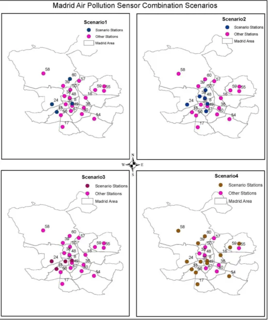
Scenario 1. Considering the AQHI established by (Stieb et al., 2008).

The AQHI defined by (Stieb et al., 2008) considers either PM10 or PM2.5. Opting to use the AQHI defined by PM10 facilitates 4 candidate sensor stations from which we can interpolate the data.

Index Sensor

Stations

AQHI(Canada) Ozone Nitrogen Dioxide PM2.5 2

CAQI(Roadside) carbon monoxide Nitrogen Dioxide PM10 PM2.5 2 CAQI(Background) carbon monoxide Ozone Nitrogen Dioxide Sulfur Dioxide PM10 PM2.5 2 DAQI(UK Defra) Ozone Nitrogen Dioxide Sulfur Dioxide PM10 PM2.5 2 Spain Madrid carbon monoxide Ozone Nitrogen Dioxide Sulfur Dioxide PM10 3 ATMO(France) Ozone Nitrogen Dioxide Sulfur Dioxide PM10 PM2.5 2

(32)

21 However, consideration of the AQHI that uses PM2.5 facilitates 2 candidate sensor stations from which data can be interpolated. The other shortcoming of this index for this study is that it was formulated with the concentration response coefficients derived from Canadian mortality data and would not represent the situation in this study area.

Scenario 2. Considering the CAQI’s Roadside index without carbon dioxide as one of the auxiliary pollutants.

Using a combination of Nitrogen Dioxide and PM10 as core pollutants with PM2.5 as an auxiliary pollutant facilitates 6 sensor stations from which data can be interpolated. Most of these stations are near the city centre of the type “Tráfico” - traffic stations. This scenario facilitates prediction of the central part of the city and not the city as a whole.

Scenario 3. Considering the CAQI’s City Background index without PM10 a core pollutant and without PM2.5 as an auxiliary pollutant.

This scenario facilitates 4 sensor stations to support interpolation though these stations are close to each other and may not give a better interpolation and representation of the entire city.

Scenario 4. Considering the CAQI’s City Background index without PM10 as a core pollutant and without auxiliary pollutants.

In this scenario where we only consider a combination of Nitrogen Dioxide and Ozone, it facilitates 14 sensor stations from which to interpolate the data. The challenge with this scenario is that we would neglect both PM2.5 and PM10, which are some of the pollutants of concern in the study area.

We present the analysed scenarios in Figure 2, with maps showing the available stations for interpolation in each scenario.

(33)

22

Figure 2: Madrid sensor stations combination scenarios

Though the Madrid AQI shares some features with the UK DAQI, Ireland’s AQHI in terms of the pollutants and the number of categories considered, there is a difference in terms of reporting as the other two indices report daily situation rather than an hourly situation reported by the Madrid AQI. This renders it challenging to compare the limit values of these indices.

The CAQI offers both hourly and daily indices but differs from the Madrid AQI in terms of the number of categories and in their formulation. The CAQI is defined by five categories against four categories of Madrid AQI and has two types of AQI, the Roadside and Background AQIs. From the formulation of these indices and considering the hourly limit values, the limit values of NO2 and PM10 for first two categories of CAQI for very low and low are the same as that of the first category of Madrid AQI with a difference in O3 limits.

(34)

23 The Madrid AQI lacks PM2.5 in its formulation yet this pollutant is among the pollutants of concern in the city and thus the need for its inclusion in an AQI formulation.

3.1.4 Formulation of the Madrid Local Air Quality Index (MLAQI)

From this study a new hourly AQI was suggested, the Madrid Local Air Quality Index (MLAQI) which was modified out of the used index in Madrid city (Madrid City Council, 2015) and uses the CAQI’s idea of core and auxiliary pollutants (Van Den Elshout, Léger and Heich, 2014). The MLAQI is based on the categories and limit values of the Madrid AQI and CAQI. The pollutants considered in this index are NO2, O3, PM10 and PM2.5. The core pollutant for MLAQI is NO2 and the auxiliary pollutants are O3, PM10 and PM2.5. With MLAQI, the index at a given station, should only be calculated with the existence of the core pollutant and at least one of O3 and PM10 pollutants. This is due to the inadequacy of PM2.5 measurements and the spatial distribution of the sensors for its measurements that would not represent the whole city while interpolated.

To get a sub index, compare a pollutant concentration with the defined limit values of that pollutant and the index range for this AQI as shown in equation (9).

𝑆_𝑥 = (𝑃𝑥− 𝑃𝑙𝑜)

(𝑃_𝑢𝑝 − 𝑃_𝑙𝑜)∗ (𝐼𝑢𝑝 − 𝐼𝑙𝑜) + 𝐼𝑙𝑜 (9)

Where 𝑆_𝑥 is the sub index, 𝑃_𝑥 is the pollutant concentration measurement, 𝑃_𝑙𝑜 is the lower limit value for the range where the pollutant measurement falls, 𝑃_𝑢𝑝 is the upper limit value for the range where the pollutant measurement falls, 𝐼𝑢𝑝is the upper limit value of the index range and

𝐼_𝑙𝑜 is the lower index limit value for the range.

To get the final index at a given sensor station which qualifies for index calculation with MLAQI, use equation (9) to calculate sub indices of the available pollutants at that station. The final index is the highest of those sub indices at that station. It is the index range which defines the category of the final index. The MLAQI is shown in Table 4 with the pollutant limit values used to calculate the sub indices and the colour coding for the respective categories.

Table 4: Madrid Local Air Quality Index

Index Range Index Category Core Pollutant

NO2 O3 PM10 PM2.5 0-50 Good 0 ‐ 100 0 ‐ 90 0-50 0-30 51-100 Acceptable 101 ‐ 200 91 ‐ 180 51-90 31-55 101-150 Poor 201 ‐ 300 181 – 240 91-150 56-90 >150 Very Poor > 300 > 240 >150 >90 Auxiliary Pollutants

(35)

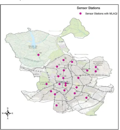
24 The strengths of this index are that it considers the local situation of Madrid city, and it considers the composition of the available sensor network and the pollutants whose concentrations can be measured. With MLAQI, the sensor network facilitates 22 out of 24 sensor stations from which we can acquire data for interpolation to represent the air quality situation in Madrid. The Figure 3 shows a map extract of the spatial distribution of the data with the defined and adopted index for the study.

Figure 3: The spatial distribution of sensor stations with MLAQI

3.1.5 Source of the routing service

With this study using the ESRI platform for implementation and the limitations with the ESRI’s routing service that limits the number of intersected streets with polygon barriers in routing, there was need for an alternative route service. We obtained this route service from the Institute of New Imaging Technologies (INIT), Universitat Jaume I (UJI) at

https://geotec.init.uji.es/arcgis/rest/services/routing/SpainNetwork/NAServer/

3.2 Implementation

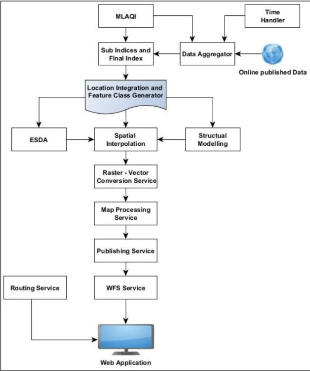
3.2.1 Implementation workflow

In using the described data to implement the study, we designed a workflow to guide the whole implementation procedure. This involved data acquisition from Madrid’s open data portal at

(36)

25

https://datos.madrid.es/portal/site/egob/, incorporation of the MLAQI, calculation of sub indices and the final indices, location integration and feature class generation, Exploratory Spatial Data Analysis (ESDA), structural modelling, spatial interpolation, raster-vector conversion, map processing, publishing a Web Feature Service (WFS) and creating routing web application. These steps support each other to reach our final goal. The followed workflow is graphically represented in Figure 4.

(37)

26

3.2.2 Data handling and implementation environment

For data retrieval, index calculation, ESDA and structural modelling, we identified a big challenge with manual data retrieval, handling and index calculation and a need for automation. This led us to creating several python modules for handling this challenge and automating the process. With the implementation in Python 2.7.12 under the ESRI ArcGIS ArcMap environment, having a limitation of requiring an active ArcMap sign in using the ArcGIS online account for publishing a WFS service. We opted for the implementation environment in Python 3.6.2 under ArcGIS Pro which integrates with the GIS python package for handling data and administration of ArcGIS online and ArcGIS for server.

3.2.3 Data acquisition, aggregation, index calculation and feature class generation

For each monitoring station, we grouped the sensors, and retrieved only the required pollutant data at every station. The data aggregation module retrieves real time and historical data, checks the data and extracts only the pollutants and their concentration values which are of interest in the study. The real time data uses the time handler module that returns the positions in the file at which the data should be queried. The time handler and data aggregation python modules are attached in appendices 7.1 and 7.2 respectively.

From the description of MLAQI, the index we have applied in the study, several considerations are needed for the index calculation. The consideration of core pollutant without which an index is not calculated for a given station and the need for at least one of the auxiliary pollutants. The index calculation module incorporates these conditions required for the index calculation at every monitoring station, checks pollutant concentrations against their limits, calculates the sub indices for only stations that meet the conditions and determines the final index from the highest sub index. The python code for the module is attached in appendix 7.3.

The feature class generator module joins the monitoring stations description and location information with the calculated index and then creates a point feature class for the support of processes like ESDA, structural data analysis and interpolation. The script for this process is contained in appendix 7.4.

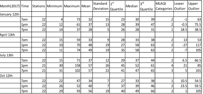
3.2.4 Exploratory Spatial Data Analysis

Before the choice of an interpolation method for this study and interpolation, we have explored our data to check for any errors, distribution and the existence of any outliers. Since the output of the interpolation was intended to serve a continuous interpolation process all the year around for

(38)

27 the real time data published by the Madrid city council, we decided to test 2017 historical data for diurnal and seasonal consistency in its behaviour. In the choice of time ranges for diurnal consistency analysis, we selected several hours of 7:00am, 1pm and 7pm for a specific day of 12th or 13th_{for the several months. For seasonal consistency analysis, we chose January, April, July and} October, which are the middle months of every season. We explored the data using the regional histogram and Voronoi polygons functionalities of ArcGIS.

3.2.5 IDW structural modelling

To analyse the data structure for modelling with IDW, we used 6 sets of different model parameters to analyse our 12 datasets. For each dataset, we first used the default parameters for modelling and recorded the model parameters together with their prediction errors. To minimise the errors in relation to equations (6) and (5), we then repeated the procedure with the other 5 sets of model parameters.

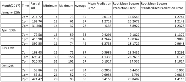
3.2.6 Variogram structural modelling

To study the structure of our data for Kriging, we employed the use of the variogram and tried fitting two different models of spherical and exponential to get an optimum one to better represent our phenomenon. The exponential model appeared to fit better our phenomenon than the spherical model and was therefore used for further structural modelling of our datasets. With the exponential model, we tried two options for all the datasets for an optimum representation. One option constituted using same model parameters for all the datasets while the other one had different model parameters for the different datasets.

With the first option using same model parameters for all the datasets except the sill, we used a nugget of 0, lag size of 2000 which was close to the Observed Mean Distance of 2417, 6 as the number of lags, 6000 as the range, 8 sectors for the sector type, 2 for minimum neighbours in a sector and 5 as the maximum neighbours in a sector. From the analysis, we recorded the values of Mean prediction error, Root Mean Square prediction error and Root Mean Square Standardised prediction error.

With the second option, we repeated the variograpy process with varying model parameters to obtain results with mean prediction error tending to 0 and Root Mean Square Standardised prediction error tending to 1. For this option, we recorded the major range, lag size, number of lags, number of neighbours, sector type and the parameters recorded in the first option.

Improving public health in smart cities in the air pollution context

Improving public health in smart cities in the air pollution

context

IMPROVING PUBLIC HEALTH IN SMART CITIES IN THE AIR POLLUTION CONTEXT

Acknowledgements

IMPROVING PUBLIC HEALTH IN SMART CITIES IN THE AIR POLLUTION CONTEXT

Abstract

Key words

Acronyms

Table of Contents

Index of tables

Index of figures

1 Introduction

1.1 Background to the study

1.2 The study area

1.3 Problem statement

1.4 Aim

1.5 Objectives

1.6 Hypothesis

1.7 Limitations

2 Literature review

2.1 Comparative study of Air Quality Indices

2.1.1 The United States Environmental Protection Agency (EPA) Air Quality Index (AQI)

2.1.2 The Canada Air Quality Health Index.

2.1.3 Common Air Quality Index (CAQI)

2.1.4 The UK Air Quality Index

2.1.5 Ireland Air Quality Index

2.1.6 Spain, Madrid Air Quality Index

2.1.7 France Air Quality Index

2.1.8 Singapore Air Quality Index

2.1.9 Researchers work on Air Quality Index representation

2.1.10 Summary of the reviewed indices

2.2 Spatial interpolation methods in air pollution

2.2.1 Spatial Interpolation

2.2.2 Deterministic and stochastic spatial interpolation methods

2.2.3 Spatial interpolation studies with air pollution

2.2.4 Summary of the used spatial interpolation methods in air pollution

2.2.5 The general prediction equation

2.2.6 Inverse Distance Weighted (IDW)

2.2.7 Kriging

2.2.8 Ordinary kriging (OK)

2.2.9 Kriging with a trend (KT)

2.2.10 The variogram or semivariogram

3 Methodology

3.1 Data description, comparison with reviewed AQIs and MLAQI formulation

3.1.1 The Madrid air pollution sensor network

3.1.2 Description of the published data from the sensor network

3.1.3 Comparison of the data with reviewed air quality indices

3.1.4 Formulation of the Madrid Local Air Quality Index (MLAQI)

3.1.5 Source of the routing service

3.2 Implementation

3.2.1 Implementation workflow

3.2.2 Data handling and implementation environment

3.2.3 Data acquisition, aggregation, index calculation and feature class generation

3.2.4 Exploratory Spatial Data Analysis

3.2.5 IDW structural modelling

3.2.6 Variogram structural modelling