1
A Work Project, presented as part of the requirements for the Award of a Master Degree in Finance from the NOVA –School of Business and Economics.
THE IMPACT OF MONETARY POLICY AND ITS SURPRISES ON BANK’S RISK-TAKING
JOÃO MIGUEL BRAVO GAUDÊNCIO* | 3241
A Project carried out on the Master in Finance Program, under the supervision of:
Professor João B. Duarte
January 2017
* To Professor João Duarte, I express my gratitude for his advices and availability, without which this project would not have been possible.
* I would also like to thank family, friends, and in particular, my dear friend Mário João Roldão, for unending hours of debate, patience, and Soviet music. Augusta per angusta.
2 Abstract
The latest financial crisis accentuated the importance of understanding bank risk and its ties to financial stability. This paper looks to investigate the impact of monetary policy in the risk-taking behaviour of Euro Area banks, when taking unconventional monetary policy into account. Looking further into this relationship, the impact of unanticipated monetary policy shocks is also analysed. Using both fixed effects and a system GMM model, sufficient statistical evidence was found to claim that looser monetary policy leads to increased risk-taking behaviour from banks. This effect, however, is mitigated in case banks and/or the market originally anticipated an even looser stance by the central bank.
JEL Codes: C23, E52, E58, G21
3 1. Introduction
The latest financial crisis, along with its underlying and unprecedented materialization of bank risk, threw into the spotlight the need for a better understanding of risk-taking behaviour and its sources, due to its abundantly clear importance for financial stability. Since then, researchers have endeavoured to find evidence linking, among others, competition (i.e. Jiménez et al. (2013)), governance (i.e. Laeven and Levine (2009)), or capital-based regulation (Dagher et al., (2016)) to bank’s risk-taking. One particular segment of that literature focuses on the impact of central banks’ monetary policy stance, often finding evidence of such a relationship. Nonetheless, an increasingly innovative monetary policy may bring about shifts in previously identified dynamics, thus creating the need for renewed assessments whenever such shifts are suspected to occur.
This paper aims to do just that, by answering two main research questions, namely: a) was the risk-taking channel of monetary policy impacted by the European Central Bank’s (ECB) usage of unconventional monetary policy; and b) what is the additional effect of unanticipated monetary policy changes, on top of the overall policy stance. The first question remains unaddressed in much of the literature as many studies focus on the low interest rate environment of the pre-Financial Crisis period, finding evidence to link those conditions with the build-up in bank risk that would lead to the eventual financial meltdown. The last question aims to take advantage of a recent strand of literature that quantifies the immediate market impact of monetary policy surprises following the ECB’s regular press conference announcements. This is relevant as a policy loosening might have a different risk-taking impact depending on whether the shift was anticipated by the market.
Using both static and dynamic panel data models to address potential data issues often raised in the literature, this paper is able to answer both questions, finding a) that a looser monetary policy stance leads, on average, to increased risk-taking behaviour from Euro Area (EA) banks,
4
even when unconventional monetary policy measures are taken into account; and b) that deviations from expectations also play a role: should monetary policy be deemed tighter than expected in a given period, then this translates to, on average, less risk-taking by EA banks, even if the overall monetary policy stance is still considered loose.
The paper is structured as follows: section 2 presents the literature review on the topic, including a more in-depth look into the innovations this project can provide; section 3 presents an overview of the data used, particularly regarding the risk-taking and monetary policy indicators to be used; section 4 presents the methodology used and the results; section 5 concludes.
2. Literature Review
i. Theoretical Literature
Since the latest Financial Crisis, considerable attention has been given to the link between monetary policy and risk build-up in the banking sector. Borio and Zhu (2008) define this so-called ‘risk-taking channel of monetary policy’ as the impact that changes in policy rates have on risk perceptions and tolerance – and, therefore, on the degree of risk in portfolios. This channel operates in three main ways. First, through the impact of interest rates on asset and collateral valuations, incomes, and cash flows. A second route involves the often-nominal nature of return rate targets; the latter exhibit a certain ‘stickiness’ which causes a ‘search-for-yield’ effect – this stickiness may stem from a contractual nature, such as with pension funds and insurance companies1, whose liabilities exhibit fixed long-term rates, or from a behavioural nature, such as the money illusion2;
1 Similarly, as Rajan (2005) illustrates, hedge fund managers also experience contractual incentives that allow for
this ‘search-for-yield’ phenomena, as their compensation is often directly linked to nominal return rate targets.
2 According to Fisher (1928), the ‘Money Illusion’ is the failure to perceive that a unit of money is capable of
expanding or shrinking in value, therefore mistaking changes in nominal value for changes in real value. The analogy here applies to a decrease in nominal yields, which may be interpreted as a decrease in real rates of return, therefore spurring higher yield demand.
5
this latter effect may be amplified by what Rajan (2005) calls a ‘herding phenomena’ – managers following their peers’ investment decisions, so as to not underperform them. The third way involves central banks’ communication policies and their reaction functions: by increasing transparency or their commitment to certain goals and decisions, uncertainty is removed, which may reduce risk premia; additionally, the belief that central banks will prevent large negative risks from materializing might lead to an asymmetrical effect – easing monetary policy will lead to more risk-taking in comparison to the reduction caused by an equivalent tightening.
Following the dot-com crash in the early 2000s, many central banks lowered interest rates to fight off recession, keeping them at historically low levels during said period, which led many to claim there is a causal link between that policy easing and the ensuing crisis. Accordingly, Delis and Kouretas (2011) describe a risk-facilitating mechanism, affirming that a prolonged period of low interest rates, and the associated decline in their volatility, releases the risk budgets of banks, allowing for higher risk positions. Gambacorta (2009) states that central banks did not take the risk build-up side of the coin into account when deciding on their policies, as they had mainly turned to tight inflation objectives – which remained stable during this period – and because of a reliance in financial innovation.3 The latter had been regarded as a factor that would strengthen the financial
system, as risk could be more efficiently allocated. Maddaloni and Peydró (2011) also go on to point out what they call the ‘low monetary rates paradox’; that is, while this risk-taking aspect facilitates the occurrence of a crisis, once it starts, central banks may lower rates again, in order to support credit supply to firms, households, and banks with weaker balance sheets, thus sowing the seeds for the next credit bubble.
3 Maddaloni and Peydró (2011) even argue that this factor amplified the impact of the low interest rate environment
6
Given these conditions, it is no wonder that the empirical literature on this subject focuses in the time frame leading up to the Financial Crisis and the years immediately following, as said period purportedly constitutes a textbook example of the inner workings of the risk-taking channel of monetary policy.
ii. Empirical Literature
Using similar methods, Gambacorta (2009), and Altunbas et al. (2009) find evidence of this channel, pointing out that banks’ risk of default seemed to increase by a larger amount in countries where interest rates had remained low for an extended period prior to the crisis. Both authors stress the need for monetary authorities to factor in the effect of their policies on risk-taking, and for supervisors to be increasingly vigilant during periods of low interest rates, particularly when the latter are coupled with fast credit and asset price increases.
Maddaloni and Peydró (2011) find evidence that low short-term interest rates have softened lending standards to both firms and households. They also find that this effect does not hold when looking at long-term interest rates, and that it is cushioned by the presence of more stringent regulatory policies on bank capital or loan-to-value (LTV) ratios.
Using loan-level data from the Spanish credit register, Jiménez et al. (2014) find that a lower overnight interest rate induces banks to grant more loan applications to ex-ante riskier firms. This effect was found to be stronger for banks with lower capitalization. Parallelly, Ioannidou et al. (2015) use the Bolivian credit register to reach similar conclusions. They find that loans with an internal subprime credit rating or loans to ex-ante riskier borrowers are more likely to be granted when rates are low. Moreover, loan spreads are not found to increase (and even seemingly decrease), which means that banks are not appropriately pricing the additional risk.
7
Andrieş et al. (2015) also reach similar results, while adding that the discovered relation is particularly negative in the post-Financial Crisis years (2008-2011). Applying a similar methodology, Pleşcău and Cocriş (2016) focus on unconventional monetary policy. They establish that the extensive use of non-standard monetary policy measures after the Financial Crisis led to increased stability for commercial banks in the EA, thus creating a higher propensity for risky activities.
Several authors find similar evidence for the US banking sector, with Dell’Ariccia et al. (2017), for instance, establishing that the risk-taking channel is more pronounced in regions that are less in sync with the nationwide business cycle, and less so for lowly capitalized banks. Furthermore, Chang and Talley (2017) report that large banks expand their off-balance sheet (OBS) activities as interest rates fall, purportedly in order to maintain shareholder value.
Delis and Kouretas (2011) postulate that the EA seems like the perfect setting for the monetary policy risk-taking channel to be identified, as the ECB pursues, unlike the Federal Reserve, price stability above any other objective. They argue that, because supervision responsibilities remain with the national competent authorities, there is little cause for thinking that financial stability is taken into account when the ECB decides on monetary policy, thus ensuring its exogeneity. It might be argued that this no longer constitutes a valid argument as, since 2014, the Single Supervisory Mechanism (SSM) has taken over supervisory duties at an EA level. Nonetheless, for the analysed time frame where this condition still holds, the authors find that a low level of interest rates positively impacts bank risk-taking, though this impact is smaller for banks with higher capital and higher for banks with more OBS items.
8
iii. Further Considerations
The present paper follows Delis and Kouretas (2011) in what regards the benefits of conducting this sort of analysis in the EA, while noting that the establishment of the SSM is not worrisome as, according to Draghi (2017), its actions have positively contributed to the effectiveness of monetary policy by ensuring that the financial system is more resilient than in the past. Therefore, the exogeneity of monetary policy is assured, since the correct identification of the risk-taking channel is not only left uncompromised, but is even assisted by this change.
Extending this analysis beyond the immediate vicinity of the Financial Crisis creates a point of divergence with previous studies, particularly for the EA, in what regards the monetary policy aspect: the incorporation of unconventional measures. Since 2015, the ECB has relied on large scale asset purchases (Quantitative Easing, or QE) and forward guidance (since 2013) to fulfil its mandate, as the zero lower bound (ZLB)4 was reached on short-term rates and conventional monetary policy was no longer able to provide further monetary stimuli. This implies that the traditional policy and short-term rates, so often used in the literature as proxies for monetary policy, no longer fully reflect the latter’s stance. The present paper uses a more comprehensive measure: the shadow rate, as proposed by Wu and Xia (2016), which takes into account the impact of such unconventional measures.
An additional novelty this project brings about is that it not only assesses the impact of the level of monetary policy, but also the influence of an unexpected monetary policy decision by the central bank on the risk-taking channel. It does so using a series of shocks constructed by Duarte and Mann (2018), following the work of Gertler and Karadi (2015). A priori, a dovish monetary
9
policy might lead to increased risk-taking – in accordance with the covered literature –, but this effect might be mitigated, should the general expectation be that the loosening would be of a larger magnitude. In this case, banks could become more cautious in anticipation of further shifts to a more hawkish central bank stance, and take on comparatively less risk.
3. Data
Financial data at the highest possible consolidation level was extracted from Standard and Poor’s market data platform, SNL5, for banks defined by the SSM, in September 2016, as
significant institutions (SI). In case an SI is owned by another same-country SI, then data is downloaded for the latter. Oftentimes, the SSM defines the holding company as the SI, and not the bank itself. For precision, should the SI hold only one bank (according to SNL), then data for that bank was downloaded. Using these criteria, an unbalanced panel with 1344 observations was created, with data obtained for 112 EA SIs, from 2005 to 2016, on a yearly basis. Quarterly data would have been preferred, in accordance with the literature, but data unavailability restricted this choice. However, in closely related research, Ashcraft (2006) and Gambacorta (2005) compare quarterly and annual data, and find that both are able to explain the impact of monetary policy rates on bank lending, thus validating annual data usage in this project. A statistical summary for all variables, along with their sources, can be found in Appendix A.1. Charts depicting the monetary policy variables’ evolution over time can be found in Appendix A.2.
i. Risk-taking variable
The existing literature on this paper’s topic employs a vast plethora of variables to identify risk-taking behaviour from banks. Gambacorta (2009) and Altunbas et al. (2009) use Moody’s
10
Expected Default Frequency (EDF), which measures the bank’s default probability in the following year. Andrieş et al. (2015), and Pleşcău and Cocriş (2016) use the Z-score, which can be understood as the bank’s distance to insolvency. Both relate to the concept of the bank’s default risk, whereas the concern here lies more on the risk of the bank’s overall portfolio. OBS activities (as in Chang and Talley (2017)) constitute a promising proxy, but data for this was not available.
Jiménez et al. (2014) and Ioannidou et al. (2015) employ a hazard model; the granularity of their data allows them to take viable ex-ante measures of credit risk such as the bank’s internal ratings for loan applications or the borrower’s credit history. However, such databases are confidential and are part of each national central bank’s credit register. Maddaloni and Peydró (2011) use the ECB’s BLS to ensure proper monetary policy identification, by isolating credit supply quality from other demand and quantity volume effects; as in the previous case, this data is confidential, and the ECB only makes country-level results public.
Delis and Kouretas (2011) use two competing risk measures: a non-performing loan (NPL) ratio and a risk-asset ratio. The former can be regarded as an ex-post measure of credit risk, as an increase in the NPL ratio in a given period does not necessarily mean that loans granted in that period were riskier, but merely that the pre-existing riskier loans have defaulted in that particular period. The risk-asset ratio is defined by the authors as ‘all assets except cash, government securities and balance due from other banks [very liquid assets, in general]; that is, all bank assets subject to a change in value due to changes in market conditions or credit quality [as a percentage of total assets]’. It constitutes a readily-available6, and arguably ex-ante measure of risk, since a ratio increase indicates that the bank has, indeed, increased its portfolio riskiness in that period,
6 These very-liquid assets are proxied in this project by the balance sheet item ‘Cash and Cash Equivalents’, which
11
based on the underlying assumptions that a) a very liquid asset is not considered to be risky; b) all illiquid assets are equally risky. This ratio constitutes, therefore, this paper’s risk-taking variable.
However, some concerns regarding the persistence of risk are present in the literature, such as in Delis and Kouretas (2011), or in Andrieş et al. (2015). The former authors point as possible causes, for instance, the effect of relationship-banking with risky borrowers, or the time required to smooth the effects of certain macroeconomic shocks which might have had an impact on risk-taking. Such persistence concerns are addressed in section 4.ii.
ii. Monetary policy variables
To measure monetary policy stances, the vast majority of the literature tends to use either a benchmark policy rate (such as the ECB’s deposit facility, or the Fed Funds Rate, in the US), a short-term rate (usually an overnight one), or a Taylor rule (à la Taylor (1993)).7 Additionally, Pleşcău and Cocriş (2016) use (alongside a Taylor Rule for conventional monetary policy) the change in level of the ECB’s balance sheet, divided by the GDP of each country as a proxy for unconventional monetary policy, following Trichet (2013).
The indicator employed here is the shadow rate, computed as described in Wu and Xia (2017), following Black (1995), who first proposed the idea of a shadow rate term structure model. His reasoning was that short-term interest rates have a ZLB because currency can be considered an option: should interest rates go below zero, then cash is preferred. Attributing the option value to the short-term rate itself, then it can be thought of as the sum of a process that allows negative rates to occur and the option value, where the latter is worth zero if short-term rates are positive.
7 A Taylor rule can be thought of as the prescribed short-term interest rate level for a given output gap and deviation
from optimal inflation. In this setting, its residuals are often used (that is, the actual rate minus the prescribed one); a negative residual indicating a loose monetary policy stance, and vice-versa.
12
Should the ZLB constraint be binding, though, then short-term rates are effectively kept at zero via the option value. In this setting, the underlying process, net of option value, is the shadow rate, which can be negative, being interpreted as the level short-term interest rates would take should the ZLB constraint not be in place.
Wu and Xia (2017) compute this shadow rate for the EA through a sophisticated state-space model, where a set of latent variables are shown to influence both the unobservable shadow rate and observable forward rates. Using the second relationship to estimate the common parameters leads to shadow rate estimates which the authors state can be used in lieu of traditional, conventional monetary policy measures. In a similar US-based study, Wu and Xia (2016) use the well-known FAVAR model, proposed by Bernanke et al. (2005), to prove that the computed shadow rate exhibits dynamic relations to key macroeconomic variables similar to the ones historically found using the effective Fed Funds Rate. A structural break was found, after the economy reached the ZLB, when using a conventional monetary policy rate, so that its use in similar settings, such as the one in this paper, is ill-advised.
A downside of shadow rates is that they are highly model-specific. Comparing two of the most widely used sets, by Krippner (2012), and the one described above, the latter is found to be less negative and volatile than the former, for instance.8 That same one is, however, made publicly available by the authors, thus being chosen, for convenience, in the lack of a predefined preference.
As mentioned before, a second monetary policy variable is also introduced, in order to account for the unexpectedness of monetary policy decisions. This variable is computed for the EA as described in Duarte and Mann (2018), following the US-based work of Gertler and Karadi
13
(2015). The authors use these shocks in a dynamic factor model to investigate their impact on the EA as a whole and on individual countries. These shocks are captured by measuring movements in the 1-year Euro Overnight Index Average (EONIA) swap rate during a six-hour period surrounding the ECB’s regular policy announcement, which takes place every six weeks. This short monitoring period intends to capture sudden appreciations or depreciations in the swap, which would then be explained purely by a potential unexpected policy shock, and not by contemporaneous changes in other macroeconomic variables, to which monetary policy could also be reacting to, thus ensuring its proper identification. This assumes that expected monetary policy was already priced into the swap before the six-hour window opens.
The full announcement includes both a short statement released to the press, with the policy decision (i.e. main rate changes, for instance), and a subsequent Q&A session, headed by the President, which may drive market expectations regarding future monetary policy actions (i.e. forward guidance). As such, the computed shock may stem from either of the two factors.
As seen in this section, the shadow rate is computed employing forward rates as a crucial methodological component. Naturally, these forward rates and, consequently, the shadow rate, are affected both by expected and unexpected monetary policy (as would any short-term rate also be). The fact that unexpected monetary policy is incorporated both into the shadow rate and the shock variable is, however, not problematic, as Duarte and Mann (2018) construct the shocks in order to render them completely exogenous to the level of monetary policy, measured here by the shadow rate. Furthermore, it is worth noting that establishing causation between the shadow rate and risk-taking can be quite troublesome, since numerous and solid control variables are required in order to assess causation, given the interconnectedness of monetary policy with macroeconomic variables. In that regard, the shock variable is able to provide a much clearer identification strategy,
14
given the aforementioned exogeneity to the monetary policy level, meaning that causation can be directly established.
iii. Control variables
This paper’s control variables are inspired by the ones used in the analysed literature and are heavily subject to data availability.9 Delis and Kouretas (2011) and Jiménez et al. (2014) define measures of bank capitalization, efficiency, and profitability. Since both papers share the same dependent variable, specifications in Delis and Kouretas (2011) are followed, defining capitalization as the equity-to-assets ratio, efficiency as the revenue-to-expenses ratio and profitability as the ratio of net profits before taxes to total assets. It should, however, be noted that Delis and Kouretas (2011) take possible endogeneity between these three variables and the risk-taking variable into account.10 Their strategy is replicated in section 4.ii.11
Bank size is also often considered to be a determinant of bank risk, and is accounted for in this paper using the natural logarithm of the bank’s total assets.
Each bank’s interest income, as a ratio of total assets, was also included into the model, in order to take, in broad terms, the bank’s business model into account (i.e. their reliance on interest income as opposed to commissions and fees). This is relevant as the mechanisms through which
9 Often-used variables in the literature that are not included in this paper were the NPL ratio, to account for the
bank’s overall risk appetite, and a concentration ratio, to account for the bank’s importance within its country.
10 The authors describe the mechanisms through which these endogenous relationships manifest themselves: i)
regarding capitalization, a bank will directly trade-off equity capital for risk assets; ii) regarding profitability, more risk assets may lead to higher/lower profits in good/bad times, which may increase/decrease the level of risk assets in the following period; iii) regarding efficiency, higher risks might explain efficiency levels in case they significantly drive bank revenue.
11 Other authors share the same strategy, due to endogeneity concerns in these, and other bank-specific variables.
15
the risk-taking channel of monetary policy manifests itself relate primarily with the interest section of a bank’s revenue.
The Basel III reforms, which brought about more stringent requirements on capital, liquidity and leverage, coming gradually into place since 2013, may have also had an impact on the risk-taking channel. Ideally, one would use a regulatory index, in the lines of Barth et al. (2004), to control for regulation stringency. The World Bank makes available a database in which such an index is computed; however, it is only available until 2011, which would be insufficient for the intended purposes. Facing this limitation, structural regulatory changes are proxied by the Capital Adequacy Ratio (CAR) (i.e. total regulatory capital over risk-weighted assets), which is a target of regulatory scrutiny.12 This identification strategy seems particularly robust, as both capitalization and the bank’s size are included in the model, which controls for changes to the CAR stemming not from regulatory shifts, but simply from fluctuations in the bank’s equity or assets. The recent liquidity regulations included in Basel III, however, are not captured by this metric.
Country-level controls are also included, such as the GDP growth rate (as in Chang and Talley (2017)), and the yearly returns on the housing market (as in Gambacorta (2009)), proxied by the yearly growth rate of each national housing market index.
12 It should be noted that the correlation between capitalization and CAR is only 0.18, thus easing possible
16 4. Methodology
i. Fixed Effects Estimator
The first approach used to tackle the problem at hands is a fixed effects model, computed as follows, in accordance with the previous section:
𝑅𝑖𝑡 = 𝛿 + 𝛼𝑀𝑃𝑡+ 𝛽𝑆ℎ𝑜𝑐𝑘𝑡+ 𝛾𝐵𝐶𝑖𝑡+ 𝜃𝐶𝐶𝑖𝑡 + 𝑢𝑖+ 𝑣𝑖𝑡 (1)
Where the 𝑖 and 𝑡 subscripts denote bank 𝑖 at time 𝑡, respectively. The dependent variable 𝑅𝑖𝑡 is the risk-asset ratio. 𝑀𝑃𝑡 denotes the monetary policy stance, given by the shadow rate, while
𝑆ℎ𝑜𝑐𝑘𝑡 represents the monetary policy shock, computed as described in section 3.ii). 𝐵𝐶𝑖𝑡 and
𝐶𝐶𝑖𝑡 are, respectively the bank-level and country-level controls. 𝑢𝑖 represents the time-invariant unobserved bank-specific effects that are not captured by the bank-level controls. 𝑣𝑖𝑡 is the traditional disturbance term, for which it is assumed that 𝑣𝑖𝑡~𝑖𝑖𝑑(0, 𝜎2). This model is estimated
using the well-known fixed effects, or within, estimator. Generalizing:
𝑦𝑖𝑡 = 𝛿 + 𝛽𝑋𝑖𝑡+ 𝑢𝑖+ 𝑣𝑖𝑡 (2)
It must be the case that:
𝑦̅𝑖 = 𝛿 + 𝛽𝑋̅𝑖+ 𝑢𝑖+ 𝑣̅𝑖 (3)
Where 𝑦̅𝑖, 𝑋̅𝑖 and 𝑣̅𝑖 refer to the averages of 𝑦𝑖𝑡, 𝑋𝑖𝑡, and 𝑣𝑖𝑡 across the time dimension 𝑡. Subtracting (3) from (2) yields:
17
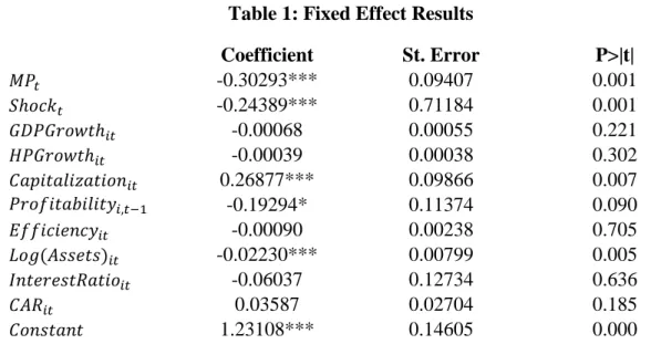
Where 𝑦̈𝑖𝑡 = 𝑦𝑖𝑡− 𝑦̅𝑖, and analogously for 𝑋̈𝑖𝑡 and 𝑣̈𝑖𝑡. This constitutes the so-called within estimator. The results obtained with this methodology can be found below, in Table 1.13 Hausman test results, which can be found in Appendix A.4., point towards fixed effects, and not random effects, as the preferred model in this context.
Table 1: Fixed Effect Results
Coefficient St. Error P>|t| -0.30293*** 0.09407 0.001 -0.24389*** 0.71184 0.001 -0.00068 0.00055 0.221 -0.00039 0.00038 0.302 0.26877*** 0.09866 0.007 -0.19294* 0.11374 0.090 -0.00090 0.00238 0.705 -0.02230*** 0.00799 0.005 -0.06037 0.12734 0.636 0.03587 0.02704 0.185 1.23108*** 0.14605 0.000
*** Significant at 1% level; ** Significant at 5% level; * Significant at 10% level
No. Observations 895 F-test (10,776) 6.72
No. Groups (Panel) 109 P>|t| 0.000
Avg. Obs. per Panel 8.2 R-Squared 0.9225
The two main variables of interest, 𝑀𝑃𝑡 and 𝑆ℎ𝑜𝑐𝑘𝑡, both exhibit significant and negative coefficients. The former was to be expected, as the reviewed literature in section 2 agrees that a looser monetary policy stance positively influences risk-taking behaviour by banks, although the effect appears quite limited: a shadow rate decrease of 1 p.p. translates, on average, into a 0.3 p.p. increase in the risk asset ratio. The second result is indicative of an adjustment to surprises in
13 Results include a constant term, which is not present in (4). The statistical software used merely reformulates (4)
based on the assumption that the average of 𝑢𝑖 across individuals is zero, in order to compute 𝛿. See Appendix B.1.
𝑆ℎ𝑜𝑐𝑘𝑡 𝐺𝐷𝑃𝐺𝑟𝑜𝑤𝑡ℎ𝑖𝑡 𝐻𝑃𝐺𝑟𝑜𝑤𝑡ℎ𝑖𝑡 𝐶𝑎𝑝𝑖𝑡𝑎𝑙𝑖𝑧𝑎𝑡𝑖𝑜𝑛𝑖𝑡 𝑃𝑟𝑜𝑓𝑖𝑡𝑎𝑏𝑖𝑙𝑖𝑡𝑦𝑖,𝑡−1 𝐸𝑓𝑓𝑖𝑐𝑖𝑒𝑛𝑐𝑦𝑖𝑡 𝐿𝑜𝑔(𝐴𝑠𝑠𝑒𝑡𝑠)𝑖𝑡 𝐶𝐴𝑅𝑖𝑡 𝐶𝑜𝑛𝑠𝑡𝑎𝑛𝑡 𝑀𝑃𝑡 𝐼𝑛𝑡𝑒𝑟𝑒𝑠𝑡𝑅𝑎𝑡𝑖𝑜𝑖𝑡
18
monetary policy. Suppose that the central bank loosens its monetary policy, but not as much as anticipated by market agents: coefficients suggest that banks take on more risk in such an instance, but that effect is mitigated by the positive (tight) surprise; if the positive shock is of 1 p.p. in the EONIA swap then, on average, the risk asset ratio can be expected to decrease by 0.2 p.p.
Intuitively, one might consider that market agents associate a ‘tight’ surprise to a higher probability of future monetary policy tightening, therefore decreasing their risk positions in anticipation. An illustrative example may be in order here: suppose the central bank keeps policy rates unchanged in their short media statement, but hints, during the subsequent Q&A session, that the interest rate regime in vigour at the time will last for a shorter period of time than originally anticipated. This would create the mentioned ‘tightening’ surprise, not simply because forward guidance was employed here, nor because it diverged from previous policy announcements, but because banks/market agents did not foresee it. As such, it is this sort of deviation from expectations is what impacts bank risk-taking.
The coefficient on the bank’s capitalization is significant and positive, which goes against the findings of Delis and Kouretas (2011) and Jiménez et al. (2014). A significant and negative coefficient is reported for the bank’s size (measured by the log of total assets), as seen in Delis and Kouretas (2011), and Bikker and Vervliet (2017); this could be a manifestation of an effect akin to ‘charter value’ theory: as a bank grows larger, its cost of failure also increases, thus incentivizing prudent behaviour.
Appendix A.5. reports a plot of the fitted values against their corresponding squared residuals, possibly hinting at the presence of heteroskedasticity. Additionally, possible persistence of the dependent variable would lead to autocorrelation in the error term; this issue is approached in the following subsection. Leaving both heteroskedasticity and autocorrelation unaccounted for
19
might lead to diminished standard errors, which would artificially inflate t-statistics. Estimating the model with heteroskedasticity- and autocorrelation-robust standard errors (Appendix A.3.) leads to no change in coefficient significance for Shockt, but 𝑀𝑃t becomes significant only at a 10% level. The same can be said for the capitalization variable, while bank size loses all significance.
ii. System GMM Estimator
As mentioned in section 3.i), concerns over the persistence of bank risk can be found in the literature. Related papers, such as Delis and Kouretas (2011), and Bikker and Vervliet (2017), address this issue by means of a dynamic panel data model (i.e., taking risk persistence into account by including a lagged dependent variable in the regressors). Both employ what is referred to as a system GMM estimator, stemming from the work of Arellano and Bond (1991) and Arellano and Bover (1995), and developed by Blundell and Bond (1998). This estimator not only allows for a dynamic setting, but also deals with the endogeneity issue described in section 3.iii), by using lags of the independent, endogenous, variables as instrumental variables (IVs) in a two 2SLS approach. It is also adequate for large N, small T datasets, such as the one used in this paper.
Including a lagged dependent variable as a regressor in a panel data model introduces what is commonly referred to as a dynamic panel bias. Said bias stems from the correlation between the lagged dependent variable and the fixed effects present in the error term14:
𝑦𝑖𝑡 = 𝛿 + 𝜌𝑦𝑖,𝑡−1+ 𝛽𝑋𝑖𝑡+ 𝜀𝑖𝑡 (5)
14 As a time-invariant parameter, 𝑢
20
Where 𝜀𝑖𝑡 = 𝑢𝑖 + 𝑣𝑖𝑡, with the latter two being defined as in (1). In fact, should the fixed effects be drawn out of the error term by means of a within estimator, this issue would still occur, since 𝑦̈𝑖,𝑡−1 would still be correlated with 𝑣̈𝑖𝑡, with the latter being computed as:
𝑣̈𝑖𝑡 = 𝑣𝑖𝑡− 1
𝑡(𝑣𝑖,𝑡−1+ 𝑣𝑖,𝑡−2+ ⋯ + 𝑣𝑖,1)
(6)
So that 𝑦̈𝑖,𝑡−1 is correlated with 𝑣̈𝑖𝑡 due to 𝑣𝑖,𝑡−1. Arellano and Bond (1991) suggest tackling
this problem by first-differencing (5). While this also expunges the fixed effects, ∆𝑦𝑖,𝑡−1 would
still be correlated with the error term ∆𝜀𝑖𝑡, through 𝜀𝑖,𝑡−1. However, longer lags do not suffer from this issue, and can thus be used as instruments, in level form.15 Alternatively, the data can be transformed through orthogonal deviations (subtracting the average of all future available observations in a panel), as proposed by Arellano and Bover (1995). This minimizes data loss, as differencing can be troublesome in a gapped panel. However, the dataset used does not exhibit such gaps and, as such, the data is transformed through differencing.
Blundell and Bond (1998) add to this, by proposing the system GMM approach: rather than instrumenting the differences with the lagged levels, the levels are instrumented with the lagged differences. However, as the fixed effects are no longer removed from the initial equation, then the lagged differences must also be uncorrelated with the fixed effects. So, for any instrument 𝑤, it must be that 𝐸(∆𝑤𝑖,𝑡−1𝑢𝑖) = 0, for any 𝑖 and 𝑡, directly implying the validity of the instrument:
𝐸(∆𝑤𝑖,𝑡−1𝜀𝑖𝑡) = 𝐸(∆𝑤𝑖,𝑡−1𝑢𝑖) + 𝐸(𝑤𝑖,𝑡−1𝑣𝑖𝑡) − 𝐸(𝑤𝑖,𝑡−2𝑣𝑖𝑡) = 0 + 0 − 0 = 0 (7)
Assuming that the 𝑣𝑖𝑡 are not serially correlated, otherwise 𝐸(∆𝑤𝑖,𝑡−1𝜀𝑖𝑡) ≠ 0, and that the
coefficient 𝜌 associated with the lagged dependent variable is below unity in absolute value.16 The
15 Instruments for the variables thought to be endogenous are not included in the instrument matrix as in a normal
2SLS approach. See Appendix B.2.
21
two-step standard error estimation described in Roodman (2009a) is implemented, as it yields heteroskedasticity-robust estimates. This standard error estimation, as well as the autocorrelation tests in Appendix A.6., relies on the assumption that errors are correlated only within individuals, not across them. A possible solution is to include time dummies, so that cross-sectional error correlation is less likely, as universal time-related shocks would be removed from the error term.
Incorporating this into the model proved unfeasible, as both 𝑀𝑃𝑡 and 𝑆ℎ𝑜𝑐𝑘𝑡 are individual-invariant, so that the full set of time dummies would perfectly predict both variables. Since the essence of the time dummies requirement is to capture those universal time-related shocks, then one can consider what would constitute such a shock, during the analyzed period, and control for it. One example would be the Financial Crisis; however, it has not affected all countries equally, let alone all banks, and its effects are already somewhat contained within the variables accounting for GDP growth and housing market returns. Another example would be recent regulatory and supervisory changes such as the introduction of the Basel III reforms, or the establishment of the SSM, as both affected all banks simultaneously. Both events are somewhat overlapping: banks started following Basel III guidelines in 2014, while the SSM was established in December of that same year. As such, given that regulatory impacts are already taken into account by the CAR, then a dummy for the establishment of the SSM was created, with the value 1 for 2015 and 2016.
The complete model is, thus:
𝑅𝑖𝑡 = 𝛿 + 𝜌𝑅𝑖,𝑡−1+ 𝛼𝑀𝑃𝑡+ 𝛽𝑆ℎ𝑜𝑐𝑘𝑡+ 𝛾𝐵𝐶𝑖𝑡+ 𝜃𝐶𝐶𝑖𝑡+ 𝜇𝑆𝑆𝑀𝑡+ 𝜀𝑖𝑡 (8)
22 Table 2: System GMM Results
Coefficient St. Error P>|t| 0.59478*** 0.05672 0.000 -0.20337*** 0.07128 0.004 -0.08444** 0.04169 0.043 0.00002 0.00033 0.962 -0.00069** 0.00028 0.012 0.33651** 0.13681 0.014 -0.35157*** 0.09259 0.000 -0.00063 0.00061 0.300 0.00206 0.00290 0.477 0.35066** 0.14343 0.014 -0.14696*** 0.03067 0.000 -0.00419** 0.00192 0.030 0.30627*** 0.05098 0.000
*** Significant at 1% level; ** Significant at 5% level; * Significant at 10% level
No. Observations 893 Wald test (𝜒132 ) 460.06
No. Groups (Panel) 109 P>|t| 0.000
Avg. Obs. per Panel 8.19 No. Instruments 52
Before delving into the discussion of results, it seems relevant to point out that the system GMM is a complex estimation technique, with many choices involved (such as the use of difference or orthogonal deviations, collapsed or non-collapsed instrument matrix17, one-step or
two-step standard error estimations, and the choice of endogenous variables). As such, reported results will be very sensitive to the model’s specifications. Therefore, results obtained from the fixed effects model may still be relevant and useful, even if stemming from a simpler approach that bypasses the issues that led to the selection of the system GMM estimator. Said output can be regarded as a guideline, against which results from a more complex model can be double-checked.
17 Only 112 panels exist, so the matrix was collapsed to restrict the number of instruments. See Appendix B.2.
𝑆ℎ𝑜𝑐𝑘𝑡 𝐺𝐷𝑃𝐺𝑟𝑜𝑤𝑡ℎ𝑖𝑡 𝐻𝑃𝐺𝑟𝑜𝑤𝑡ℎ𝑖𝑡 𝐶𝑎𝑝𝑖𝑡𝑎𝑙𝑖𝑧𝑎𝑡𝑖𝑜𝑛𝑖𝑡 𝑃𝑟𝑜𝑓𝑖𝑡𝑎𝑏𝑖𝑙𝑖𝑡𝑦𝑖,𝑡−1 𝐸𝑓𝑓𝑖𝑐𝑖𝑒𝑛𝑐𝑦𝑖𝑡 𝐿𝑜𝑔(𝐴𝑠𝑠𝑒𝑡𝑠)𝑖𝑡 𝐶𝐴𝑅𝑖𝑡 𝑀𝑃𝑡 𝐼𝑛𝑡𝑒𝑟𝑒𝑠𝑡𝑅𝑎𝑡𝑖𝑜𝑖𝑡 𝑅𝑖,𝑡−1 𝐶𝑜𝑛𝑠𝑡𝑎𝑛𝑡 𝑆𝑆𝑀𝑡
23
As a first result, the lagged dependent variable is indeed significant, confirming the notion that bank risk, or at least the risk-asset ratio, is a persistent variable. It should be noted that the coefficient is, however, significantly smaller than one, which validates the model. The two main coefficients, for the 𝑀𝑃𝑡 and 𝑆ℎ𝑜𝑐𝑘𝑡 variables, remain statistically significant and negative, in line with results from section 4.i. This time around, a shadow rate decrease of 1 p.p. translates, on average, into a 0.2 p.p. increase in the risk asset ratio. Regarding 𝑆ℎ𝑜𝑐𝑘𝑡, an increase of 1 p.p. in
the EONIA swap due to a monetary policy surprise, on average, tends to lead to a decrease by 0.1 p.p. in the risk-asset ratio.
Similar results to the fixed effects model could not be found for the bank size coefficient, which is no longer significant. Capitalization, however, retains its positive and significant coefficient. The interest income ratio and the CAR are both significant in explaining the risk-asset ratio, with a positive and negative coefficient, respectively. A higher reliance on interest should, indeed, imply a higher risk asset ratio, as loans would be more common place, when compared to OBS activities, which would be more prevalent should the bank rely more on commissions and fees, and do not contribute to the ratio. Stricter regulation, here measured by the CAR, should also lead to lower risk-taking by banks, as Maddaloni and Peydró (2011) demonstrate.
The returns on the national house price indexes are also significant with a negative sign, contradicting the results of Gambacorta (2009). Profitability, once-lagged, also exhibits a significant and negative coefficient, which contradicts the theory proposed by Delis and Kouretas (2011), that higher profitability is a precursor to increased risk-taking behavior in the following period. It should, however, be noted that the same authors could not find significance for this variable in their study. The SSM dummy also exhibits a significant and negative coefficient, indicating that the introduction of EA-level supervision successfully mitigated risk-taking.
24
The model’s validity is confirmed by the test results found in Appendix A.6. The Arellano-Bond test for autocorrelation in first differences points rejects the null hypothesis of no first-order autocorrelation. This is an expected outcome, as the test is conducted on differenced errors, so that ∆𝜀𝑖𝑡 is necessarily correlated with ∆𝜀𝑖𝑡−1 through 𝜀𝑖𝑡−1. Rather, the problematic first-order autocorrelation in the levels (which would render lags of the dependent variable invalid as instruments) would be reflected in the second-order autocorrelation for the differences, for which an identical null hypothesis is not rejected.
The Hansen test of overidentifying restrictions finds no statistical evidence that the instruments are correlated with the error term, and thus does not reject the null hypothesis of joint validity of all instruments.18 Following advice from Roodman (2009b), difference-in-Hansen tests were also computed for four different subsets of instruments19: a) instruments pertaining to the
endogenous regressors; b) instruments for the dependent variable; c) instruments for the exogenous regressors (which instrument themselves); and d) the subset consisting of a + b. All tests validate the choice of instruments.
5. Conclusion
The present paper is able to find evidence that banks’ risk-taking in the EA is positively impacted by a looser monetary policy stance by the ECB. This result seems to fall perfectly in line with previous research conducted on this risk-taking channel. The period analysed here allows for the ECB’s unconventional monetary policy measures to be taken into account. This is accomplished using a shadow rate as the main monetary policy measure, rather than a short-term,
18 The Sargan test, which assumes homoskedasticity, is also reported and not rejected. See Appendix A.6.
19 These test not only for the exogeneity of the particular subset, but also for a critical assumption regarding the
25
or a main policy rate. Value is also added to the literature by identifying what is the additional impact of a surprising policy announcement by the ECB. These shocks are quantified by measuring changes in 1-year EONIA swap rates in a small period around the ECB’s routine monetary policy press conference. A ‘tightening’ shock, for instance, seems to lead to a reduction in risk.
These results were found to be robust to potentially endogenous variables, and to persistence in the dependent variable, as a system GMM was employed following an initial fixed effects approach. Both strategies yield consistent results for the main variables of interest, although the shadow rate coefficient is not significant when estimating fixed effects with heteroskedasticity-robust standard errors. However, the methodology could be benefit from access to a more comprehensive database, which would allow for further bank-level control variables, which are crucial for correctly identifying the true impact of monetary policy on the dependent variable.
Since the accumulation of bank risk often has a nefarious impact on financial stability, conclusions found in this, and similar papers, can play into the recent debate on whether or not monetary policy decisions should take financial stability considerations into account (through an augmented Taylor rule that would take the latter into account, for instance). Indeed, macroprudential authorities have already started advocating for such a change in paradigm, and this paper’s findings certainly reinforce their cause. Naturally, such a shift would require a more exhaustive assessment of its potential impacts, which are duly addressed in the relevant literature, and are out of the scope of this project.
26 References
Altunbas, Y., Gambacorta, L., and Marqués-Ibáñez, D. (2009). “Bank Risk and Monetary Policy”. ECB Working Paper Series, No 1075.
Andrieş, A., Pleșcău, I., and Cocriș, V. (2015). “Low Interest Rates and Bank Risk-Taking: Has the Crisis Changed Anything? Evidence from the Eurozone”. Review of Economic & Business Studies, Volume 8, Issue 1.
Arellano, M. and Bond, S. (1991). “Some Tests of Specification for Panel Data: Monte Carlo Evidence and an Application to Employment Equations”. The Review of Economic Studies, Volume 58, Issue 2.
Arellano, M. and Bover, O. (1995). “Another Look at the Instrumental Variable Estimation of Error-Component Models”. Journal of Econometrics, Volume 68, Issue 1.
Ashcraft, A. (2006). “New Evidence on the Lending Channel”. Journal of Money, Credit, and Banking, Volume 38, No. 3.
Barth, J., Caprio, G., and Levine, R. (2014) “Bank Regulation and Supervision: What Works Best?”, Journal of Financial Intermediation, Volume 13, Issue 2.
Bernanke, B., Boivin, J., and Eliasz, P. (2005). “A Factor Augmented Vector Autoregressive Approach”. The Quarterly Journal of Economics, Volume 120, No. 1.
Bikker, J. and Vervliet, T. (2017). “Bank Profitability and Risk-Taking under Low Interest Rates”. DNB Working Paper, No.560.
27
Blundell, R. and Bond, S. (1998). “Initial Conditions and Moment Restrictions in Dynamic Panel Data Models”. Journal of Econometrics, Volume 87, Issue 1.
Borio, C. and Zhu. H. (2008). “Capital Regulation, Risk-Taking and Monetary Policy: a Missing Link in the Transmission Mechanism?”. BIS Working Papers, No. 268.
Chang, Y. and Talley, D. (2017). “Bank Risk in a Decade of Low Interest Rates”. Journal of Economics and Finance, Volume 41, Issue 3.
Dagher, J., Dell’Ariccia, G., Laeven, L., Ratnovski, L., and Tong, H. (2016) “Benefits and Costs of Bank Capital”. IMF Staff Discussion Note, No.16/04.
Delis, M. and Kouretas, G. (2011). “Interest Rates and Bank Risk-Taking”. Journal of Banking and Finance, Volume 5, Issue 4.
Dell’Ariccia, G., Laeven, L., and Suarez, G. (2017). “Bank Leverage and Monetary Policy's Risk‐ Taking Channel: Evidence from the United States”. The Journal of Finance, Volume 72, Issue 2. Draghi, M. (2017). “The Interaction Between Monetary Policy and Financial Stability in the Euro Area”. Keynote speech at the First Conference on Financial Stability. Madrid, May 2017.
Duarte, J. and Mann, S. (2018). “A Dynamic Factor Model with High-Frequency Identification for Monetary Policy in the Euro Area”. University of Cambridge Working Paper.
Fisher, I. (1928). “The Money Illusion”. New York: Alephi Company.
Gambacorta, L. (2005). “Inside the Bank Lending Channel”. European Economic Review, Volume 49, Issue 7.
Gambacorta, L. (2009). “Monetary Policy and the Risk-Taking Channel”. BIS Quarterly Review, 2009/12.
28
Gertler, M. and Karadi, P. (2015). “Monetary Policy Surprises, Credit Costs, and Economic Activity”. American Economic Journal: Macroeconomics, Volume 7, Issue 1.
Hakkio, C. and Kahn, G. (2014). “Evaluating Monetary Policy at the Zero Lower Bound”, The Macro Bulletin, Kansas City Federal Reserve Bank, 2014/07.
Ioannidou, V., Ongena, S., and Peydro, J. (2015). “Monetary Policy, Risk-Taking, and Pricing: Evidence from a Quasi-Natural Experiment”. Review of Finance, Volume 19, Issue 1
Jiménez, G., Ongena, S., Peydró, J., and Saurina, J. (2014). “Hazardous Times for Monetary Policy: What Do Twenty-Three Million Loans Say About the Effects of Monetary Policy on Credit Risk-Taking?”. Econometrica, Volume 82, No. 2.
Jiménez, G. and Saurina, J. (2013). “How Does Competition Affect Risk-Taking?”. Journal of Financial Stability, Volume 9, Issue 2.
Krippner, L. (2012). “Modifying Gaussian Term Structure Models When Interest Rates are Near the Zero Lower Bound”. Reserve Bank of New Zealand Discussion Papers, 2012/02.
Laeven, L. and Levine, R. (2009). “Bank Governance, Regulation and Risk Taking”. Journal of Financial Economics, Volume 93, Issue 2.
Lombardi, M. and Zhu, F. (2014). “A Shadow Policy Rate to Calibrate US Monetary Policy at the Zero Lower Bound”. BIS Working Paper, No. 452.
Maddaloni, A. and Pedyró, J. (2011). “Bank Risk-Taking, Securitization, Supervision and Low Interest Rates”. ECB Working Paper Series, No. 1248.
Nickell, S. (1981). “Biases in Dynamic Models with Fixed Effects”. Econometrica, Volume 49, Issue 1.
29
Pleșcău, I. and Cocriș, V. (2016). “Unconventional Monetary Policy and Bank Risk Taking in the Euro Area”. Ovidius University Annals, Series Economic Sciences, Volume 16, Issue 1.
Rajan, R. (2005). “Has Financial Development Made the World Riskier?”. NBER Working Paper, No.11728.
Roodman, D. (2009a). “How to do xtabond2: An Introduction to Difference and System GMM in Stata”. The Stata Journal, Volume 9, No. 1.
Roodman, D. (2009b). “A Note on the Theme of Too Many Instruments”. Oxford Bulletin of Economics and Statistics, Volume 71, Issue 1.
Swanson, E. (2017). “Measuring the Effects of Federal Reserve Forward Guidance and Asset Purchases on Financial Markets”, NBER Working Papers, No. 23311
Taylor, J. (1993). “Discretion Versus Policy Rules in Practice”. Carnegie-Rochester Conference Series on Public Policy, Volume 39, Issue 1.
Trichet, J. (2013). “Unconventional Monetary Policy Measures: Principle – Conditions – Raison d’Être”. International Journal of Central Banking, Volume 9, No. 1.
Wu, J.C. and Xia, F.D. (2016). “Measuring the Macroeconomic Impact of Monetary Policy at the Zero Lower Bound”. Journal of Money, Credit and Banking, Volume 48, Issue 2-3.
Wu, J.C. and Xia, F.D. (2017). “Time-Varying Lower Bound of Interest Rates in Europe”. Chicago Booth Research Paper, No. 17-06.