3 With the benefit of hindsight, we will try to

António Afonso, António Jorge Silva

The Monetary Transmission Mechanism in the Euro

Area: has it changed with the EMU? A VAR

approach, with fiscal policy and financial stress

considerations

WP10/2014/DE/UECE _________________________________________________________

De pa rtme nt o f Ec o no mic s

W

P

The Monetary Transmission Mechanism in the Euro

Area: has it changed with the EMU? A VAR approach,

with fiscal policy and financial stress considerations

António Afonso

, António Jorge Silva

June 2014

Abstract

We study whether the adoption of the Euro and a single monetary policy have brought about a change in the monetary transmission mechanism and between the interactions of monetary policy, fiscal policy and financial stress in the Euro area. We find that the stylized facts of monetary transmission remain valid, but the response of output and, especially, fiscal and financial stress variables to a monetary policy shock, seems to be stronger in the post-EMU period. Regarding fiscal and financial stress shocks, the inclusion in the post-EMU period of subprime and sovereign debt crises yields, changes, not only in the scale, but also in the patterns of the responses of our model’s main variables.

JEL codes: E42, E44, E52, E58, E63

Keywords: monetary transmission mechanism, fiscal policy, financial stress, Euro area, vector autoregressions

*

The opinions expressed herein are those of the authors and do not necessarily reflect those of the Banco de Portugal, the European Central Bank or the Euro system.

$

ISEG/ULisboa – Universidade de Lisboa, Department of Economics; UECE – Research Unit on Complexity and Economics, R. Miguel Lupi 20, 1249-078 Lisbon, Portugal, email: aafonso@iseg.utl.pt. UECE is supported by the Fundacão para a Ciência e a Tecnologia (Portuguese Foundation for Science and Technology) through the PEst-OE/EGE/UI0436/2011 project, European Central Bank, Directorate General Economics, Kaiserstraße 29, D-60311 Frankfurt am Main, Germany.

#

1

1.

Introduction

On December 31st, 1998, the conversion rates between the 11 participating national currencies and the Euro were fixed. On the following day, January 1st, 1999, the Euro became the official currency of the 11 countries in Europe1, and a single monetary policy was introduced under the authority of the European Central Bank (ECB).

Adopting the Euro as a single currency was a culmination point of several decades of economic and financial integration between European countries, and it marked the third and final stage of the Economic and Monetary Union (EMU).2

However, since the beginning of the process that led to the establishment of a single currency in Europe, there has been extensive discussion as to whether a single monetary policy would be suitable for the countries that adhere to the Euro, considering their differences in economic, financial and social structures.

For some time, such fundamental discussion took place mostly amongst academic and political circles in Europe and also in the USA. However, with the recent advent of the sovereign debt crisis in Europe after the 2008-2009 subprime crises, this discussion is ever more present in the common European citizen’s everyday talk. Therefore, the referred culmination point may not be the final word on monetary integration in Europe and further developments are to be expected.

One of the fundamental aspects of the Euro, is the existence of a single monetary policy for the Euro area, conducted under the authority of the ECB. The Monetary Transmission Mechanism (MTM) is the process through which monetary policy affects real variables and prices in the economy and thus the understanding of this mechanism is pivotal to examining the single monetary policy under the ECB.

15 years have now passed the adoption of the Euro, and 12 years since the entry into circulation of Euro coins and banknotes.3 With the benefit of hindsight, we will try to

1

The eleven founding countries of the Euro were: Austria, Belgium, Finland, France, Germany, Ireland, Italy, Luxembourg, the Netherlands, Portugal and Spain. Since then, other countries have adopted the Euro: Greece joined in 2001, Slovenia in 2007, Cyprus and Malta in 2008, Slovakia in 2008, Estonia in 2011 and Latvia in 2014.

2

2

assess whether the adoption of a single monetary policy has brought about a change in the MTM of the Euro area. Our perspective is Euro area wide and we will use a quarterly data sample from Q1 1987 to Q4 2011, to study the transmission mechanism pre, and post, Euro. The methodological approach will be a vector auto regression (VAR) model.

Furthermore, bearing in mind the impact of the subprime financial crisis and the sovereign-debt crisis in the Euro area in more recent years, we study at a macro-level the interactions between monetary policy, fiscal policy and stress in the financial sector for the area as a whole.

The rest of the paper is structured as follows: Section 2 presents the related literature; Section 3 reviews the econometric framework; Section 4 presents the data, the variables and the empirical results and Section 5 concludes.

2.

Related literature

2.1. Monetary Transmission Mechanism related VARs

The process of establishing a single currency in Europe has, since the very beginning, generated ample discussions amongst economists as to whether a single monetary policy would be suitable for the countries that adhere to the Euro, and as to what could be the impacts of such a single policy. The economic literature on the MTM in Europe can be divided in two main approaches. One approach focuses on the MTM of the individual countries of the Euro area, i.e., on a country by country basis. Other studies follow an area wide perspective, i.e., they study the transmission mechanism of the Euro area as a whole. Both approaches have been used to analyze the transmission mechanism prior to, and after, Stage Three of the EMU.4

In 1999, the ECB launched a research initiative to study the transmission of monetary policy in the Euro area. Angeloni et al. (2003a) have an overall compilation of

3

For the first three years, the Euro was only used for accounting purposes and did not have a physical existence. The Euro coins and banknotes were introduced in 1 January 2002.

4

3

several papers that were produced with this aim, and in Angeloni et al. (2003b) a complete summary and discussion of the main findings is provided.

Following the ECB’s initiative, around the turn of the century, several authors focused their research on uncovering the stylized facts of the MTM in Europe and, in some cases, attempted to envisage the consequences for such mechanism of a single monetary policy. For instance, Mojon and Peersman (2003), following a country by country approach, find that the effects of monetary policy on GDP and prices were broadly similar in the individual countries of the Euro area. This indicates that monetary policy transmission might be similar between those countries before the EMU. Guiso et al. (1999) focus on whether a common monetary policy for the Euro area would have asymmetrical effects in the different countries and have a good literature overview on the topic. They report some significant differences across countries in several indicators that may matter for monetary transmission, even if no definitive conclusion seemed to be possible at the time. Peersman (2004) provides a comprehensive review of pre-EMU literature on cross-country comparisons.

Smets and Peersman (2003), following an area-wide approach, find that a temporary rise in the nominal and real short-term interest rate tended to be followed by a real appreciation of the exchange rate, a temporary fall in output and that prices seemed to be more sluggish and only started to fall significantly below zero, several quarters after changes in GDP. Reassuringly, these results were very similar to those obtained for the US economy, using similar methodologies.

In recent years, researchers have begun to assess monetary policy by the ECB, that is, the single monetary policy in the Euro area after 1999. This has been possible because the common monetary policy in the Euro area is now about 15 years old, therefore, using the latest available data, econometric studies based on time series are now starting to become more robust.

4

evidence for a second one around 1999, concluding that monetary transmission after 1998 is not very different from that of before 1996, but probably very different compared to the interim period of 1996 - 1999, which is indicative of a possible period of adjustment, prior to the Euro. Moreover, they find that the stylized facts of monetary policy transmission remain valid. Boivin, Giannoni and Mojon (2009) report important heterogeneity across countries5 in the effect of monetary shocks before the launch of the Euro and conclude that the creation of the Euro has contributed to a greater homogeneity of the transmission mechanism across countries and an overall reduction in the effects of monetary shocks.

In the past couple of years, various authors included the subprime crisis period in their analysis and, in some instances, the more recent sovereign debt crisis. However, these analyses are mostly focused on the effects of the unconventional monetary policy measures that have been taken since.6

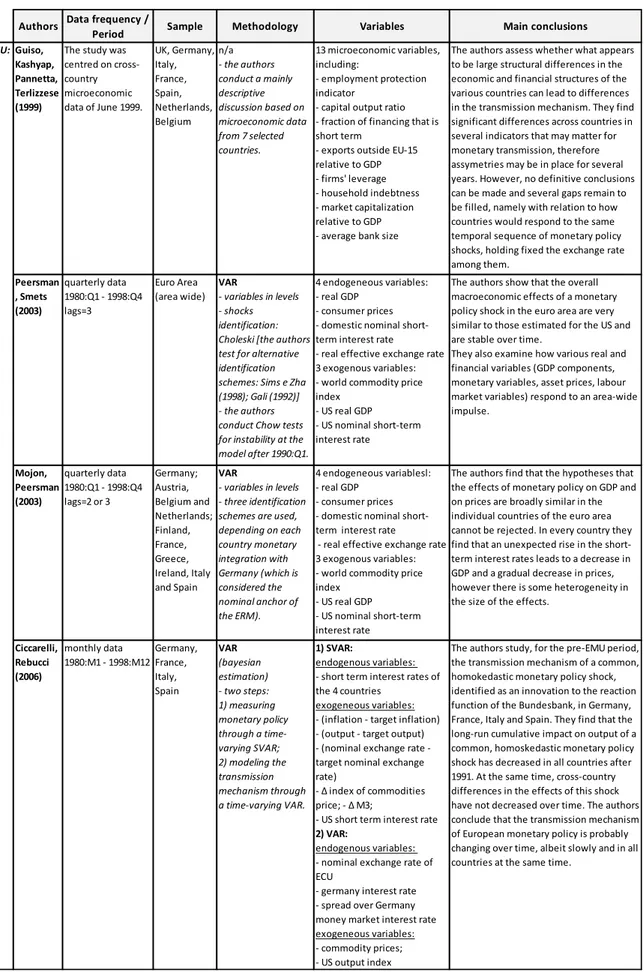
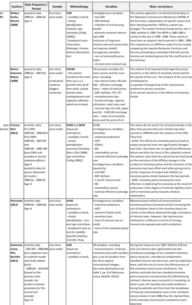
Tables 1 and 2 present a brief systematic summary of the empirical literature on the MTM, pre, and post-EMU. We identify the period of the analysis, the sample, the methodology, the variables included in the empirical models and then, finally, the main conclusions.

Regarding methodology, the seminal work of Sims (1980) was the precursor for the use of VAR models for the analysis of monetary policy and these models have been, and still are, a widely used framework for the study of the MTM. VAR models provide an empirical method for capturing the dynamic relations between economic variables (time series), without the need to impose rigid identification restrictions. This characteristic of the framework allows for more flexibility and less a priori theorization.

5

The authors constructed a FAVAR, using data from the six largest countries of the Euro area.

6

5

Table 1 – Related literature overview (pre-EMU sample)

Authors Data frequency /

Period Sample Methodology Variables Main conclusions

Pre-EMU: Guiso, Kashyap, Pannetta, Terlizzese (1999)

The study was centred on cross-country microeconomic data of June 1999.

UK, Germany, Italy, France, Spain, Netherlands, Belgium n/a

- the authors conduct a mainly descriptive discussion based on microeconomic data from 7 selected countries.

13 microeconomic variables, including:

- employment protection indicator

- capital output ratio - fraction of financing that is short term

- exports outside EU-15 relative to GDP - firms' leverage - household indebtness - market capitalization relative to GDP - average bank size

The authors assess whether what appears to be large structural differences in the economic and financial structures of the various countries can lead to differences in the transmission mechanism. They find significant differences across countries in several indicators that may matter for monetary transmission, therefore assymetries may be in place for several years. However, no definitive conclusions can be made and several gaps remain to be filled, namely with relation to how countries would respond to the same temporal sequence of monetary policy shocks, holding fixed the exchange rate among them.

Peersman , Smets (2003)

quarterly data 1980:Q1 - 1998:Q4 lags=3

Euro Area (area wide)

VAR

- variables in levels - shocks identification: Choleski [the authors test for alternative identification schemes: Sims e Zha (1998); Gali (1992)] - the authors conduct Chow tests for instability at the model after 1990:Q1.

4 endogeneous variables: - real GDP

- consumer prices - domestic nominal short-term interest rate

- real effective exchange rate 3 exogenous variables: - world commodity price index

- US real GDP

- US nominal short-term interest rate

The authors show that the overall macroeconomic effects of a monetary policy shock in the euro area are very similar to those estimated for the US and are stable over time.

They also examine how various real and financial variables (GDP components, monetary variables, asset prices, labour market variables) respond to an area-wide impulse.

Mojon, Peersman (2003)

quarterly data 1980:Q1 - 1998:Q4 lags=2 or 3

Germany; Austria, Belgium and Netherlands; Finland, France, Greece, Ireland, Italy and Spain VAR

- variables in levels - three identification schemes are used, depending on each country monetary integration with Germany (which is considered the nominal anchor of the ERM).

4 endogeneous variablesl: - real GDP

- consumer prices - domestic nominal short-term interest rate

- real effective exchange rate 3 exogenous variables: - world commodity price index

- US real GDP

- US nominal short-term interest rate

The authors find that the hypotheses that the effects of monetary policy on GDP and on prices are broadly similar in the individual countries of the euro area cannot be rejected. In every country they find that an unexpected rise in the short-term interest rates leads to a decrease in GDP and a gradual decrease in prices, however there is some heterogeneity in the size of the effects.

Ciccarelli, Rebucci (2006)

monthly data 1980:M1 - 1998:M12

Germany, France, Italy, Spain VAR (bayesian estimation) - two steps: 1) measuring monetary policy through a time-varying SVAR; 2) modeling the transmission mechanism through a time-varying VAR.

1) SVAR:

endogenous variables: - short term interest rates of the 4 countries

exogeneous variables: - (inflation - target inflation) - (output - target output) - (nominal exchange rate - target nominal exchange rate)

- Δ index of commodities price; - Δ M3;

- US short term interest rate 2) VAR:

endogenous variables: - nominal exchange rate of ECU

- germany interest rate - spread over Germany money market interest rate exogeneous variables: - commodity prices; - US output index

6

Table 2 – Related literature overview (including post-EMU sample)

Authors Data frequency /

Period Sample Methodology Variables Main conclusions Post-EMU: Weber, Gerke, Worms (2009) quarterly data 1980:Q1 - 2006:Q4 lags=2

Euro Area (area wide)

VAR

- variables in levels - shocks identification: Choleski; sign restriction [Uhlig (2005)]; - breakpoint tests: Chow tests; Ploberger, Kramer, Kontrus fluctuation test.

4 endogeneous variables: - real GDP

- GDP deflator - indicator of real housing wealth

- domestic nominal interest rate (3M)

(inclusion of long term interest rate and money does not improve model) 2 exogenous variables: - non-oil commodity price index

- US short term interest rate

The authors approach is to identify break dates in the Monetary Transmission Mechanism (MTM) of the Euro Area, independent of specific causes and then checking whether MTM as a whole has changed. The authors find two break points, one in 1996, another in 1999. The MTM in 1980-1996 is similar to the one in 1999 - 2006. There seems to have been an atypical interim period in 1996 - 1999. The comparisons on MTM are made first by visually comparing the Impulse Response Functions and then by estimating an extended VAR with period dummy and conducting tests for the coefficients of the dummys. Boivin, Giannoni, Mojon (2009) quarterly data 1980:Q1 - 2007:Q3 lags=3 Euro Area (area wide) + 6 individual countries (biggest countries) FAVAR

- the authors transform the series - they use y-o-y growth rates of all time series, except interest rates, unemployment and capacity utilization which are in levels.

33 economic variables for each country and the euro area, including:

- two interest rates, M1 and M3; - effective exchange rates; - index of stock prices - GDP, deflator, PPI, CPI - unemployment rate - hourly earnings, capacity utilization, retail sales and: - interest rates for USA, Japan and UK; - EUR/USD exchange rate; - index of commodity prices and the price of oil.

The authors find important heterogeneity across countries in the effect of monetary shocks before the launch of the euro. The creation of the euro has contributed to:

1) a greater homegeneity of the transmission mechanism accross countries;

2) an overall reduction in the effects of monetary shocks. after subprime: Cecioni, Neri (2011)

monthly data: Pre-EMU: 1994:M1 - 1998:M12 Post-EMU: 1999:M1 - 2007:M7 and

1999:M1 - 2009: M9 (post EMU sub-samples to test for subprime effects) lags=4 quarterly data (to assess robustness of results): 1989:Q1 - 2009:Q2 lags=3

Euro Area (area wide)

SVAR and DGSE

(bayesian estimation)

- variables in levels - shocks identification: recursive (Choleski); Sims e Zha (1999); sign restrictions [Uhlig (2005)].

SVAR:

6 endogeneous variables: (monthly)

- industrial production - HICP

- EONIA; - M2

- commodities prices - nominal effective exchange rate

6 endogeneous variables: (quarterly)

- real GDP - GDP deflator - 1 month interest rate; - M2

- commodities prices - nominal effective exchange rate

The autors do not search for structural breaks in the data, they assume that such a break may have ocurred in 1999:M1 with the creation of the EMU. They find:

- SVAR: The effects of a monetary policy shock on output and prices have not significantly changed over time. Also there are no significant differences before and after the burst of the subprime turmoil. The authors claim that this cannot be the final word on the evolution of the MTM as changes in the conduct of monetary policy and the structure of the economy may have offset each other giving rise to similar responses of output and inflation to monetary policy shocks between the two periods. - DGSE: monetary policy has become more effective in stabilizing the economy as the result of a decrease in the degree of nominal rigidities and a shift in monetary policy towards inflation stabilization.

Peersman (2011)

monthly data 1999:M1 - 2009:M2 lags=4 Euro Area (area wide) SVAR (bayesian estimation) - variables in levels - shocks identification: zero and sign restrictions - breakpoint tests to test for stability: Quandt-Andrews, CUSUM, Chow.

6 endogeneous variables: - industrial production - HICP

- volume of bank credit - monetary base - level of interest rate on credit

- level of the monetary policy rate

Macroeconomic effects of unconventional monetary policies (characterized by increasing the size of balance sheet or the monetary base) are similar to the effects obtained through innovations of interest rates. However, the transmission mechanism is different in terms of timings, interest rate spreads and credit multipliers.

Giannone, Lenza, Phil, Reichlin (2011) monthly data . 1991:M1 - 2008:M8

(pre-subprime crisis to estimate model and study stilized facts)

. 1999:M1 - 2010:M3

(based on the previous time sample, the authors estimate previsions for this second sub-sample) lags=13 Euro Area (area wide) VAR (bayesian estimation)

- variables in levels.

39 variables, including: - macroeconomic, financial, monetary and credit variables plus a set of variables from the US to capture international linkages. (for more detail please see table 1, pp. 6 of Giannone, Lenza, Reichlin (2012))

During the financial crisis 2007-2010 the ECB not only cut interest rates significantly but also introduced a package of non-standard monetary policy measures, intended to complement standard interest rate decisions, and not substitute them, with the aim to insure the effectiveness of the monetary transmission mechanism. The authors conclude that non-standard monetary policy measures introduced by the ECB following

Lehman’s demise were successful in insulating, at

7

2.2. Fiscal policy, monetary policy and financial instability

The effects of monetary policy on macroeconomic aggregates have been studied broadly, mainly by using VAR frameworks, or the New Keynesian DSGE models and some stylized facts have been identified as we have mentioned previously. Particularly for the Euro area, researchers have then turned their focus to the impact of the EMU on those stylized facts, and, more recently, on the functioning of the different transmission channels during the subprime and the sovereign debt crisis, as well as the effects of the unconventional monetary policy response to the crises.

Conversely, when it comes to the effects of fiscal policy on macroeconomic aggregates, there are no stylized facts, i.e., there are no facts which are broadly agreed upon. The difficulties start on the basics: how to distinguish between a change in revenues and expenditures, caused by automatic stabilizers and a deliberate fiscal policy change. Afonso et al. (2011) present a comprehensive review of fiscal policy VAR-related literature and they point out the different results that often arise when different identification schemes are used and also in cross-country samples.

For instance, Afonso et al. (2011) use a Threshold VAR to study the effects of fiscal policy in high financial stress regimes and low financial stress regimes. They find that the response of economic growth to fiscal shocks is generally positive in both financial stress regimes and that financial stress has a negative effect on output growth and that it increases the government debt-to-GDP ratio. Their country sample7 also indicates that the initial conditions, such as, the existence of financial stress, diverse levels of government indebtedness and implicit monetary policy, are relevant in determining the nonlinearities that were found regarding the effects of a fiscal shock on economic activity.

Interactions between financial system stress and monetary policy are also relevant. Stress in the banking sector, stock markets and exchange rate markets may play important roles in the transmission of monetary policy shocks.8 For example, Baxa et al.

7

They estimate a TVAR for the US, UK, Germany and Italy.

8

8

(2013) conclude that central banks, when faced with high financial stress, often alter the course of monetary policy, mainly by lowering interest rates and also that the size of the response varies overtime, as well as across countries.9 They also report some cross-country heterogeneity with regard to the effects of specific types of financial stress.

3.

Econometric framework

To analyze the effects of a monetary policy shock in the Euro area, we use a VAR model with the following representation:

[1] Zt = A(L)Zt-1 + μt,

where Zt is the vector of endogenous variables, and ut is the vector of serially

uncorrelated disturbances that have a zero mean and a time invariant covariance matrix.

A(L) denotes a polynomial matrix in the lag operator. We also include a constant in the model.

The vector of endogenous variables in our benchmark model consists of six Euro area variables: real GDP growth (yt), inflation (pt), annual change in the debt-to-GDP

ratio (ft), long-term nominal interest rate (lt), short-term nominal interest rate (it) and a

financial stress indicator (st):

[2] Z t’= [yt pt ft lt it st].

The inclusion of a debt sustainability indicator (proxied by the debt-to-GDP ratio) and a measure of financial stress, although not common in the monetary policy VAR related literature, will hopefully allow us to incorporate in the dynamics of our model two variables that historically, and possibly more markedly in (recent) times of economic and financial distress, may influence the Monetary Transmission Mechanism.10

We identify the monetary policy shocks by assuming a recursive (Choleski) structure. The variables are ordered as in [2], which reflects some assumptions

9

Their sample includes the US, UK, Australia, Canada and Sweden.

10

9

regarding the links between the economic variables. Specifically, we assume that the monetary policy shocks (i.e., the changes in short-term nominal interest rate –it) do not

have a contemporaneous impact on output, prices, debt-to-GDP ratio and long term interest rates, but that they may contemporaneously affect the financial stress indicator. On the other hand, the policy interest rate does not respond to contemporaneous changes in the financial stress indicator. The ordering of the fiscal variable before output, follows Afonso et al. (2011), and is justified by the need to identify the effects of automatic stabilizers on the economy. The financial stress indicator is ordered last, which implies that it reacts contemporaneously to all variables in the system.

The lag length of the endogenous variables, Zt, is an important aspect of the

estimation procedure, as, if the lag length is too small, then the model may be wrongly specified and if it is too long, then degrees of freedom are being lost. The usual lag length selection criteria are presented in appendix A.3. The tests results indicate one lag for the Schwarz information criteria (SC) and two lags for Akaike (AIC) and Hannan-Quinn (HQ) information criteria. The Akaike criteria may overestimate the lags, but the SC and HQ are consistent for small samples (Lutkepohl (2005)). We opt for one lag, mainly because the limited number of observations in the pre and post-EMU sub-samples could impair the estimation of a six variable VAR, should more lags be considered.

4.

Empirical analysis

4.1The data and variables

We estimate the VAR model using quarterly data from Q1 1987 to Q4 2011. The source for the Euro area wide macroeconomic time-series was the 12th update of the Area-Wide Model (AWM) database11

, except for the case of the government debt for the Euro area, which was retrieved from the Quarterly Fiscal database for the Euro

11

10

area.12 The financial stress index that we use for the Euro area, is the Composite Indicator of Systemic Stress (CISS),proposed by Halló et al. (2012)13, and the data was made available by the ECB. The time sample is limited, due to data availability. In particular, the CISS time series only starts in 1987 and the data from the latest available update of the AWM database stops in Q4 2011.

For real GDP and the GDP deflator, we use the annual growth rates of the logs. For the debt-to-GDP ratio we use the annual change in the ratio. These transformations allow us to sidestep the known non-stationary characteristics of the original levels variables. Real GDP, GDP deflator and debt-to-GDP ratio are all seasonally adjusted. The monetary policy instrument is a three month nominal interest rate, as in Fagan et al. (2001). For CISS we computed the quarterly averages of weekly values.14

4.2 Overview of macroeconomic, monetary, fiscal and financial developments15

The average year-on-year growth rate of real GDP for the Euro in our sample was 1.9%. During these 25 years there were two very marked recessions, the first one was in 1993 and the second and deeper recession was in 2008-2009. Furthermore, smaller growth rates were observed in 2002-2003 and after the second Quarter of 2011.

Regarding the annual change in the GDP deflator (our proxy for inflation), and long and short term interest rates, there has been a change in the levels of these variables, in the sense that, during the 90s, there was a decrease in the values from the considerable high levels observed in the end of the 1980s to more or less stabilized lower levels from 1998 onwards.

12

For a description of the database, please see Paredes et al. (2009). We use Euro Area general government debt, and then calculate the debt-to-GDP ratio, using the GDP provided in the AWM database. The resulting series has a very good match with the Eurostat debt-to-GDP ratio series for the Euro area, available only with data after Q1 2000.

13

The CISS is an indicator of contemporaneous stress in the financial system, proposed by Halló et al.

(2012). Its main goal is to “measure the (…) current level of frictions, stresses and strains (or the absence of these) in the financial system and to condense that state of financial instability into a single statistic” (idem). It is a composite indicator, focused on the systemic dimension of financial stress, and comprises

the five most important segments of an economy’s financial system: bank and non-bank financial intermediaries, money markets, securities (equities and bonds) markets and foreign exchange markets. For more details on the construction of the CISS, please refer to Halló et al. (ibidem).

14

In Appendix A.1 we present all the data and sources, in a systematic manner.

15

11

The debt-to-GDP ratio for the Euro area has increase at a steady pace from just below 60% in 1987, to around 75% in 1996. From 1996 to 2008, the ratio has declined somewhat, attaining a level of 67% in 2008. After 2008, and related notably to the government’s response to the subprime crisis and also to the need to capitalize the banking sector, there was a very sharp increase in the debt-to-GDP ratio, which at the end of 2010 had already climbed to 86% of GDP. During 2011, the ratio continued to increase, albeit at a slower pace, closing the year at 88%.

Finally, concerning the Composite Indicator of Systemic Stress - our financial stress variable – we can observe a prolonged period of very high stress in the Euro area from Q3 2007 until the end of our sample in Q4 2011 (with slight improvements in Q3 2010 and Q4 2010). The very high financial stress in this period is, on the one hand, due to the subprime crisis, whose first signs appeared during 2007 - namely with the decision by BNP Paribas on the 9th of August, 2007, to stop the bail-out of three funds by BNP Paribas that were affected by the subprime problems - and was compounded by the failure of Lehman Brothers on the 15th of September, 2008, resulting in the highest historical levels of CISS in Q4 2008 and Q1 2009. On the other hand, from the end of 2009 onwards, the high levels of financial stress are mainly justified by the sovereign debt crises in Europe that followed the subprime crises. The first signs appeared on the yields of Greek sovereign bonds, whose rise led to the joint financial assistance program

12

4.3Empirical results

We are interested in investigating whether there have been changes in the MTM, in association with the adoption of the Euro and also in the interactions between monetary and fiscal policy. To that end, we consider two balanced samples: the first sub-sample refers to the years prior to the adoption of the Euro, and runs from Q1 1987 to Q4 1998; the second sub-sample includes the post-Euro adoption years – Q1 1999 to Q4 2011. The aim is to inspect the respective impulse response functions (IRFs) and to detect any differences that may exist between them.16

Furthermore, we also explore the relevance of additional sub-samples, namely, a subprime and a sovereign debt crisis sub-sample. In order to do so, we exclude from the post-EMU sub-sample the final years - which correspond to the periods of these two crises.

Our VAR model includes two macroeconomic policy variables – interest rate and debt-to-GDP ratio – and a financial stress variable. Therefore, it can be used to study the interactions of fiscal and monetary policy, on one hand, and of these two macro variables with financial stress, on the other hand. It is possible to study these interactions in our framework by basically analysing the impact of monetary shocks on the fiscal variable, as well as the impact of fiscal shocks on the interest rate and also the impact of financial stress on both variables (as well as on all the other non-policy related variables in our VAR).

4.3.1 The effects of interest rates shocks

The complete set of responses of the variables to the (negative) monetary shock, for all sub-samples, is shown in appendix A.4. The solid line depicts the median response estimate and the dashed lines show the two-standard error confidence intervals. For all sub-samples considered, the one-standard deviation monetary policy shock is estimated

16

13

to be around 30 basis points, which is in line with the estimate obtained by Peersman and Smets (2003).

Comparing the pre-EMU and post-EMU sub-samples, we can observe a stronger response of the main macro-economic variables to a negative interest rate shock (i.e., a temporary increase in the short-term interest rate) in the post-EMU sub-sample. In particular, the output growth reacts more negatively in the first 8 to 10 Quarters, and then the recuperation of output growth occurs at a faster pace. Although there are differences in the amplitude of output growth response, the time frames over which these responses develop does not seem to differ significantly between the two sub-samples - whilst in the pre-EMU sub-sample, the output growth turns positive after around 14 Quarters and in the post-EMU sub-sample, such recovery occurs after 12 Quarters.

With regards to inflation, there seems to be a somewhat bigger price-puzzle17 in the post-EMU sub-sample, than in the pre-EMU sub-sample. The negative response of inflation to an increase in interest rate seems to be of a similar scale, although in the pre-EMU period, the response is somewhat more prolonged in time.

Concerning the response of the fiscal variable, we observe a much higher increase in the debt-to-GDP ratio after a negative interest rate shock in the post-EMU sub-sample, than in the pre-EMU sub-sample. In fact, the increase in the annual change of the debt-to-GDP ratio in the second sub-sample more than doubles that of the first sub-sample. The same pattern holds for the financial stress response – a negative monetary policy shock has a much higher impact on the financial stress variable in the post-EMU sub-sample, than in the pre-EMU sub-sample.

Overall, the changes in the responses of our VAR variables in the post-EMU sub-sample are more significant for the fiscal and financial stress variables, than for output growth and inflation. These changes may be a consequence of a higher degree of synchronization of the Euro area countries’ economies after the adoption of the Euro.

17

14

However, if we exclude the Quarters after the beginning of the subprime crises from the post-EMU sub-sample , i.e., if our post-EMU sub-sample stops at Q2 2007, then IRFs are of a much smaller magnitude18 and, also, there is a very considerable price-puzzle. As Peersman (2011) concluded, the policy response to the recession after the subprime crises seems to have improved the identification of conventional monetary policy shocks. In our paper we can further corroborate that this may have been the case, because our sub-sample which excludes the sovereign debt crisis, yields results that are much similar to the full sample results. Therefore, it was the subprime crises’ period,

and not the sovereign debt crises’ period that contributed to improving the identification of conventional monetary policy shocks.

4.3.2 The effects of fiscal shocks

The complete set of responses of the variables to the positive fiscal shock, for all sub-samples, is shown in Appendix A.5. If we compare the period of Q1 1987 – Q4 1998 to the period of Q1 1999–Q4 2011, the changes in the IRFs of our variables to a fiscal shock are substantial, not only in magnitude, but also in the directions of the responses. For instance, the response of output growth to a positive fiscal shock in the second sub-sample is negative in the first few quarters, whilst such an answer is positive in the pre-EMU sub-sample.

These changes may be related to the Governments’ answer to the subprime recession

– after the subprime crises there was a steep increase in governments’ debt-to-GDP ratio and this increase was accompanied by a deep recession. This idea is supported by the following: if we look at the estimates of the one-standard deviation fiscal policy shock, we conclude that such a shock was estimated to be around 0.3 percentage points (p.p.) in the pre-EMU period, but its estimate rose to more than 0.5 p.p. in the post-EMU sub-sample. However, if we exclude the subprime period (and the sovereign debt crises

18

Boivin et al. (2009) also find an overall reduction in the effects of monetary shocks after 1999, using a sample that does not include the subprime crises (their sample stops in Q3 2007). They conclude that

15

period) – i.e., if we consider the Q11999- Q2 2007 sub-sample – the estimate of a one-standard deviation fiscal policy shock comes down to just over 0.2 p.p.. The lower-than-average real GDP growth, and higher-than-lower-than-average annual increase in debt-to-GDP ratio that characterise the sovereign debt crises, may also be importantly related to the change in direction of the output growth response to a fiscal shock.

In the pre-EMU sub-sample, the long-term interest rate responds with a steady increase to a positive fiscal shock, whilst the short-term interest rate responds with a slight decrease in the first few Quarters, followed by a prolonged increase. In the pos-EMU sub-sample, both the short-term and long-term interest rate responses are negative in the first few Quarters, and then turn to slightly positive territory after about 15 Quarters, albeit the scale of the fall, and posterior rise, of short term interest rate is comparatively higher. Therefore, a positive fiscal shock seems to be followed by a steepening of the yield curve in the short run, for both sub-samples.

4.3.3 The effects of financial stress shocks

The complete set of responses of the variables to financial stress shock, for all sub-samples, is shown in Appendix A.6. As expected, the shocks are considerably higher in the post-EMU sub-sample, if we include the subprime and the sovereign debt crisis period. In the full post-EMU sub-sample, the one-standard deviation financial stress shock is estimated at around 45 points, whilst for the pre-EMU and post-EMU except subprime sub-samples, the estimates are similar, at around 30 points.

16

On the contrary, if we include the period of the subprime crises in the post-EMU sub-sample (i.e., if we consider the period Q1 1999- Q4 2009), then there has been a clear change in the magnitude and pattern of responses, with output growth responding in a strong and negative fashion to the shock, and debt-to-GDP responding with a strong increase in its annual change. Furthermore, including the sovereign debt crises period (i.e., considering the whole post-EMU period – Q1 1999 to Q4 2011) increases the negative response of output growth to the financial stress shock. Lastly, there is a positive response of the long term interest rate to a financial stress shock in all of the post-EMU sub-samples, which did not exist in the pre-EMU sub-sample.

4.4. Robustness check: an alternative pre-EMU sub-sample

Weber et al. (2009) found that there may have been a significant break point in the monetary mechanism period in the Euro area around 1996 and also some evidence for a second one around 1999, suggestive of an interim period from Q2 1996 to Q4 1998 of adjustment, prior to the Euro. Following that conclusion we estimate a VAR from Q1 1981 to Q1 1996 and also the respective IRFs and then compare them with the post-EMU sub-samples.

17

5.

Conclusions

The adoption of the Euro and of a single monetary policy might have contributed to changing the monetary transmission mechanism and the interactions between monetary policy, fiscal policy and financial stress in the Euro area.

Our results indicate that the stylised facts of monetary transmission remain valid, but the response of output and, especially, of the fiscal and financial stress variables to an increase in the short term interest rate, seems to be stronger in the post-EMU period. These changes may be a consequence of a higher degree of synchronization of the Euro

area countries’ economies after the adoption of the Euro. However, if we exclude the subprime crises from the post-EMU period, then the sizes of the responses are much smaller. Our results support Peersman’s (2011) conclusion that policy response to the subprime recession seems to have improved the identification of conventional monetary policy shocks.

In addition, regarding fiscal and financial stress shocks, the inclusion in our post-EMU sub-sample of the subprime and sovereign debt crises yields, changes in the scale, and also in the patterns of the responses of the main variables of our model. For instance, there is a very strong increase in the debt-to GDP ratio following a financial stress shock in the post-EMU period, whilst such a response was negative in the pre-EMU period. Another important feature is the small magnitude of the IRFs of the post-EMU period, when we exclude the subprime and sovereign debt crises.

18

References

Afonso, A., J. Baxa and M. Slavik (2011), Fiscal developments and financial stress: a threshold VAR analysis, ECB Working Paper No. 1319.

Angeloni, I., A. Kashyap and B. Mojon (eds.) (2003), Monetary Transmission in the Euro Area, Cambridge University Press.

Angeloni, I., A. Kashyap, B. Mojon and D. Terlizzese (2003), Monetary Transmission in

the Euro Area: were do we stand?, in Monetary policy transmission in the Euro area, I.

Angeloni, A. Kashyap and B. Mojon (eds), Cambridge University Press, Chapter 24.

Apel, E. (1998), European Monetary Integration 1958 – 2002, Routledge.

Baxa, J., R Horváth and B. Vasícek (2013), Time-varying monetary-policy rules and

financial stress: does financial instability matter for monetary policy?, Journal of Financial

Stability, Issue 9.

Boivin, J., M. P. Giannoni and B. Mojon (2009), How has the Euro changed the monetary

transmission?, in NBER Macroeconomics Annual 2008, Vol. 23, National Bureau of

Economic Research.

Boivin, J., M. Kiley and F. Mishkin (2010), How has the transmission mechanism evolved over time?, NBER Working paper No. 15879.

Ciccarelli, M. and A. Rebucci (2006), Has the transmission mechanism of European

monetary policy changed in the run-up to EMU?, European Economic Review, Vol. 50, No.

3.

Cecioni, M. and S. Neri (2011), The monetary transmission mechanism in the Euro area:

has it changed and why?, Banca d’Italia Working Paper No. 808.

Fagan, G., J. Henry and R. Mestre, (2001), An area wide (AWM) model for the Euro area, Working Paper 42, ECB Working Paper No. 42.

Gali, J. (1992), How well does the IS-LM model fit postwar US data?, Quarterly Journal of

Economics, May, Vol. 107, No. 2

Giannone, D., M. Lenza, H. Phill and L. Reichlin (2011), Non-standard monetary policy measures and monetary developments, ECB Working Paper No. 1290.

Giannone, D., M. Lenza and L. Reichlin (2012), Money, Credit, Monetary Policy and the Busines Cycle in the Euro Area, ECARES Working Paper.

Guiso, L., A. Kashyap, F. Panetta and D. Terlizzese (1999), Will a Common European

Monetary Policy Have Asymmetric Effects?, Economic Perspectives 4, Federal Reserve

19

Halló, D., M. Kremer and M. L. Duca (2012), CISS - A Composite Indicator of Systemic Stress in the Financial System, ECB Working Paper No. 1426.

Lutkeppohl, H. (2005), New Introduction to Multiple Time Series Analysis, Springer.

Lutkeppohl, H. (2011), Vector Autoregressive Models, Economics Working Papers ECO 2011/30, European University Institute.

Mojon, B. and G. Peersman (2003), A VAR description of the effects of monetary policy in

the individual countries of the Euro area, in Monetary policy transmission in the Euro area,

I. Angeloni, A. Kashyap and B. Mojon (eds), Cambridge University Press, Chapter 3.

Paredes, J., D. Pedregal and P. Jávier (2009), A Quarterly Fiscal database for the Euro Area based on intra-annual fiscal information, ECB Working Paper No. 1132.

Peersman, G. and F. Smets (2003), The monetary transmission mechanism in the Euro area:

more evidence from VAR analysis, in Monetary policy transmission in the Euro area, I.

Angeloni, A. Kashyap and B. Mojon (eds), Cambridge University Press, Chapter 2.

Peersman, G. (2004), The transmission of monetary policy in the Euro Area: are the effects

different across countries?, Oxford Bulletin of Economics and Statistics, Vol. 66, No.3.

Peersman, G. (2011), Macroeconomic effects of unconventional monetary policy in the Euro Area, ECB Working Paper No. 1397.

Sims, C. (1980), Macroeconomics and Reality, Econometrica, Vol. 48, No. 1.

Sims, C., J. Stock and M. Watson (1990), Inference in Linear Time Series Models With

Some Unit Roots, Econometrica, Vol. 58, No. 1.

Sims, C. and T. Zha (1998), Bayesian methods for dynamic multivariate models,

International Economic Review, Vol. 39, No. 4.

Sims, C. and T. Zha (1999), Error bands for impulse responses, Econometrica, Vol. 67, No.

5.

Uhlig, H. (2005), What are the effects of monetary policy on output? Results from an

agnostic identification procedure, Journal of Monetary Economics, Vol. 52.

Ungerer, H. (1997), A Concise History of European Monetary Integration – from EPU to

EMU, Praeger.

20

Appendix

A. 1 - Data description and sources

Variables in the VAR model:

yt GDP, annual growth rate of the log of the real GDP (Y) used: yt = log(Yt) - log(Yt-4).

pt Price level (P), annual growth rate of logs used: pt = log(Pt) - log(Pt-4).

lt Long term interest rate. it Short-term interest rate.

ft Annual change in the debt to GDP ratio: ft = Ft - Ft-4.

st Financial stress index (CISS), quarterly averages of weekly values.

Sources:

A. 2 – Data on the variables used in the VAR

Variables Data Sources Periodicidade Time sample

availabitlity

Seasonally

adjusted? Series ID Euro Zone

Yt GDP (real)

Area Wide Model Database

- 12th update quarterly 1980Q1-2011Q4 Yes YER

Pt GDP deflator

Area Wide Model Database

- 12th update quarterly 1980Q1-2011Q4 Yes YED

lt Long term interest rate (nominal)

Area Wide Model Database

- 12th update quarterly 1980Q1-2011Q4 LTN

it Short term interest rate (nominal)

Area Wide Model Database

- 12th update quarterly 1980Q1-2011Q4 STN

Ft Debt/GDP

Quarterly Fiscal Database -

ECB quarterly 1980Q4-2012Q4 Yes MAL

St

Composite Indicator of Systemic

Stress ECB weekly 1987-2013 CISS

-4 0 4 8 12

88 90 92 94 96 98 00 02 04 06 08 10

annual chang e i n debt- to- g dp r ati o

0 2 4 6 8 10 12 14

88 90 92 94 96 98 00 02 04 06 08 10

short term interest rate

2 4 6 8 10 12

88 90 92 94 96 98 00 02 04 06 08 10

long ter m interest rate

0 1 2 3 4 5 6

88 90 92 94 96 98 00 02 04 06 08 10

defl ator infl ation

0 200 400 600 800

88 90 92 94 96 98 00 02 04 06 08 10

financial stress indicator (ciss)

-6 -4 -2 0 2 4 6

88 90 92 94 96 98 00 02 04 06 08 10

21 A. 3 – Lag selection criteria

VAR Lag Order Selection Criteria

Endogenous variables: Y P F L I S Exogenous variables: C

Sample: 1987Q1 - 2011Q4 Included observations: 96

Lag AIC SC HQ

0 28.94277 29.10304 29.00755

1 16.42683 17.54874* 16.88033

2 15.76005* 17.84359 16.60225*

3 15.85670 18.90186 17.08760

4 15.99905 20.00584 17.61866

* indicates lag order selected by the criterion

22 A. 4 – Effects of interest rates shocks

Pre-EMU sub-sample: Q1 1987 – Q4 1998 Post-EMU sub-sample: Q1 1999 – Q4 2011

-.6 -.4 -.2 .0 .2 .4

2 4 6 8 10 12 14 16 18 20 22 24

Response of Y to I

-.3 -.2 -.1 .0 .1 .2

2 4 6 8 10 12 14 16 18 20 22 24

Response of P to I

-.6 -.4 -.2 .0 .2 .4

2 4 6 8 10 12 14 16 18 20 22 24

Response of F to I

-.6 -.4 -.2 .0 .2 .4

2 4 6 8 10 12 14 16 18 20 22 24

Response of L to I

-.8 -.6 -.4 -.2 .0 .2 .4

2 4 6 8 10 12 14 16 18 20 22 24

Response of I to I

-5 0 5 10 15

2 4 6 8 10 12 14 16 18 20 22 24

Response of S to I

Response to Cholesky One S.D. Innovations ± 2 S.E.

-.8 -.4 .0 .4

2 4 6 8 10 12 14 16 18 20 22 24

Response of Y to I

-.2 -.1 .0 .1

2 4 6 8 10 12 14 16 18 20 22 24

Response of P to I

-1.0 -0.5 0.0 0.5 1.0 1.5

2 4 6 8 10 12 14 16 18 20 22 24

Response of F to I

-.2 -.1 .0 .1

2 4 6 8 10 12 14 16 18 20 22 24

Response of L to I

-.6 -.4 -.2 .0 .2 .4

2 4 6 8 10 12 14 16 18 20 22 24

Response of I to I

-40 -20 0 20 40 60 80

2 4 6 8 10 12 14 16 18 20 22 24

Response of S to I

23

Post-EMU, pre-subprime crisis sub-sample: Q1 1999 – Q2 2007 Post-EMU, pre-sovereign debt crisis sub-sample: Q1 1999 – Q4

2009 -.3 -.2 -.1 .0 .1 .2

2 4 6 8 10 12 14 16 18 20 22 24

Response of Y to I

-.08 -.04 .00 .04 .08 .12

2 4 6 8 10 12 14 16 18 20 22 24

Response of P to I

-.3 -.2 -.1 .0 .1 .2 .3

2 4 6 8 10 12 14 16 18 20 22 24

Response of F to I

-.20 -.15 -.10 -.05 .00 .05 .10

2 4 6 8 10 12 14 16 18 20 22 24

Response of L to I

-.3 -.2 -.1 .0 .1 .2 .3

2 4 6 8 10 12 14 16 18 20 22 24

Response of I to I

-15 -10 -5 0 5 10

2 4 6 8 10 12 14 16 18 20 22 24

Response of S to I Response to Cholesky One S.D. Innovations ± 2 S.E.

-.6 -.4 -.2 .0 .2 .4 .6

2 4 6 8 10 12 14 16 18 20 22 24

Response of Y to I

-.4 -.3 -.2 -.1 .0 .1 .2

2 4 6 8 10 12 14 16 18 20 22 24

Response of P to I

-1.0 -0.5 0.0 0.5 1.0

2 4 6 8 10 12 14 16 18 20 22 24

Response of F to I

-.3 -.2 -.1 .0 .1 .2

2 4 6 8 10 12 14 16 18 20 22 24

Response of L to I

-.6 -.4 -.2 .0 .2 .4 .6

2 4 6 8 10 12 14 16 18 20 22 24

Response of I to I

-40 -20 0 20 40

2 4 6 8 10 12 14 16 18 20 22 24

24 Alternative pre-EMU sub-sample: Q1 1987 – Q1 1996

-.6 -.4 -.2 .0 .2 .4

2 4 6 8 10 12 14 16 18 20 22 24

Response of Y to I

-.3 -.2 -.1 .0 .1 .2

2 4 6 8 10 12 14 16 18 20 22 24

Response of P to I

-.3 -.2 -.1 .0 .1 .2 .3 .4

2 4 6 8 10 12 14 16 18 20 22 24

Response of F to I

-.3 -.2 -.1 .0 .1 .2

2 4 6 8 10 12 14 16 18 20 22 24

Response of L to I

-.6 -.4 -.2 .0 .2 .4

2 4 6 8 10 12 14 16 18 20 22 24

Response of I to I

-5 0 5 10 15 20

2 4 6 8 10 12 14 16 18 20 22 24

25 A. 5 – Effects of fiscal shocks

Pre-EMU sub-sample: Q1 1987 – Q4 1998 Post-EMU sub-sample: Q1 1999 – Q4 2011

-.2 -.1 .0 .1 .2 .3

2 4 6 8 10 12 14 16 18 20 22 24

Response of Y to F

-.4 -.2 .0 .2 .4 .6

2 4 6 8 10 12 14 16 18 20 22 24

Response of P to F

-.4 -.2 .0 .2 .4 .6 .8

2 4 6 8 10 12 14 16 18 20 22 24

Response of F to F

-0.8 -0.4 0.0 0.4 0.8 1.2

2 4 6 8 10 12 14 16 18 20 22 24

Response of L to F

-0.8 -0.4 0.0 0.4 0.8 1.2

2 4 6 8 10 12 14 16 18 20 22 24

Response of I to F

-8 -4 0 4 8 12

2 4 6 8 10 12 14 16 18 20 22 24

Response of S to F

Response to Cholesky One S.D. Innovations ± 2 S.E.

-.8 -.4 .0 .4

2 4 6 8 10 12 14 16 18 20 22 24

Response of Y to F

-.2 -.1 .0 .1

2 4 6 8 10 12 14 16 18 20 22 24

Response of P to F

-0.8 -0.4 0.0 0.4 0.8 1.2

2 4 6 8 10 12 14 16 18 20 22 24

Response of F to F

-.20 -.15 -.10 -.05 .00 .05 .10

2 4 6 8 10 12 14 16 18 20 22 24

Response of L to F

-.6 -.4 -.2 .0 .2 .4

2 4 6 8 10 12 14 16 18 20 22 24

Response of I to F

-40 -20 0 20 40 60 80

2 4 6 8 10 12 14 16 18 20 22 24

26

Post-EMU, pre-subprime crisis sub-sample: Q1 1999 – Q2 2007 Post-EMU, pre-sovereign debt crisis sub-sample: Q1 1999 – Q4

2009 -.3 -.2 -.1 .0 .1 .2 .3

2 4 6 8 10 12 14 16 18 20 22 24

Response of Y to F

-.10 -.05 .00 .05 .10

2 4 6 8 10 12 14 16 18 20 22 24

Response of P to F

-.3 -.2 -.1 .0 .1 .2 .3

2 4 6 8 10 12 14 16 18 20 22 24

Response of F to F

-.12 -.08 -.04 .00 .04 .08 .12

2 4 6 8 10 12 14 16 18 20 22 24

Response of L to F

-.2 -.1 .0 .1 .2

2 4 6 8 10 12 14 16 18 20 22 24

Response of I to F

-15 -10 -5 0 5 10

2 4 6 8 10 12 14 16 18 20 22 24

Response of S to F Response to Cholesky One S.D. Innovations ± 2 S.E.

-.3 -.2 -.1 .0 .1 .2 .3 .4

2 4 6 8 10 12 14 16 18 20 22 24

Response of Y to F

-.1 .0 .1 .2 .3

2 4 6 8 10 12 14 16 18 20 22 24

Response of P to F

-.6 -.4 -.2 .0 .2 .4 .6

2 4 6 8 10 12 14 16 18 20 22 24

Response of F to F

-.1 .0 .1 .2 .3 .4

2 4 6 8 10 12 14 16 18 20 22 24

Response of L to F

-.2 -.1 .0 .1 .2 .3 .4 .5

2 4 6 8 10 12 14 16 18 20 22 24

Response of I to F

-30 -20 -10 0 10 20 30

2 4 6 8 10 12 14 16 18 20 22 24

27 Alternative pre-EMU sub-sample: Q1 1987 – Q1 1996

-.4 -.3 -.2 -.1 .0 .1 .2 .3

2 4 6 8 10 12 14 16 18 20 22 24

Response of Y to F

-.3 -.2 -.1 .0 .1 .2

2 4 6 8 10 12 14 16 18 20 22 24

Response of P to F

-.3 -.2 -.1 .0 .1 .2 .3 .4

2 4 6 8 10 12 14 16 18 20 22 24

Response of F to F

-.3 -.2 -.1 .0 .1 .2

2 4 6 8 10 12 14 16 18 20 22 24

Response of L to F

-.6 -.4 -.2 .0 .2 .4 .6

2 4 6 8 10 12 14 16 18 20 22 24

Response of I to F

-20 -15 -10 -5 0 5 10

2 4 6 8 10 12 14 16 18 20 22 24

28 A. 6 – Effects of financial stress shocks

Pre-EMU sub-sample: Q1 1987 – Q4 1998 Post-EMU sub-sample: Q1 1999 – Q4 2011

-.4 -.2 .0 .2 .4 .6

2 4 6 8 10 12 14 16 18 20 22 24

Response of Y to S

-.4 -.2 .0 .2 .4

2 4 6 8 10 12 14 16 18 20 22 24

Response of P to S

-.8 -.4 .0 .4

2 4 6 8 10 12 14 16 18 20 22 24

Response of F to S

-1.2 -0.8 -0.4 0.0 0.4 0.8

2 4 6 8 10 12 14 16 18 20 22 24

Response of L to S

-1.0 -0.5 0.0 0.5 1.0

2 4 6 8 10 12 14 16 18 20 22 24

Response of I to S

-10 0 10 20 30 40

2 4 6 8 10 12 14 16 18 20 22 24

Response of S to S Response to Cholesky One S.D. Innovations ± 2 S.E.

-1.00 -0.75 -0.50 -0.25 0.00 0.25 0.50

2 4 6 8 10 12 14 16 18 20 22 24

Response of Y to S

-.3 -.2 -.1 .0 .1 .2

2 4 6 8 10 12 14 16 18 20 22 24

Response of P to S

-0.8 -0.4 0.0 0.4 0.8 1.2 1.6

2 4 6 8 10 12 14 16 18 20 22 24

Response of F to S

-.1 .0 .1 .2

2 4 6 8 10 12 14 16 18 20 22 24

Response of L to S

-.6 -.4 -.2 .0 .2 .4

2 4 6 8 10 12 14 16 18 20 22 24

Res pons e of I to S

-40 0 40 80

2 4 6 8 10 12 14 16 18 20 22 24

29

Post-EMU, pre-subprime crisis sub-sample: Q1 1999– Q2 2007 Post-EMU, pre-sovereign debt crisis sub-sample: Q1 1999 – Q4

2009 -.3 -.2 -.1 .0 .1 .2 .3

2 4 6 8 10 12 14 16 18 20 22 24

Response of Y to S

-.15 -.10 -.05 .00 .05 .10

2 4 6 8 10 12 14 16 18 20 22 24

Response of P to S

-.4 -.3 -.2 -.1 .0 .1 .2 .3

2 4 6 8 10 12 14 16 18 20 22 24

Response of F to S

-.10 -.05 .00 .05 .10 .15 .20

2 4 6 8 10 12 14 16 18 20 22 24

Response of L to S

-.2 -.1 .0 .1 .2 .3

2 4 6 8 10 12 14 16 18 20 22 24

Response of I to S

-10 0 10 20 30 40

2 4 6 8 10 12 14 16 18 20 22 24

Response of S to S Response to Cholesky One S.D. Innovations ± 2 S.E.

-.8 -.4 .0 .4 .8

2 4 6 8 10 12 14 16 18 20 22 24

Response of Y to S

-.3 -.2 -.1 .0 .1 .2 .3 .4

2 4 6 8 10 12 14 16 18 20 22 24

Response of P to S

-1.0 -0.5 0.0 0.5 1.0

2 4 6 8 10 12 14 16 18 20 22 24

Response of F to S

-.2 -.1 .0 .1 .2 .3 .4

2 4 6 8 10 12 14 16 18 20 22 24

Response of L to S

-.4 .0 .4 .8

2 4 6 8 10 12 14 16 18 20 22 24

Response of I to S

-60 -40 -20 0 20 40 60

2 4 6 8 10 12 14 16 18 20 22 24

30 Alternative pre-EMU sub-sample: Q1 1987 – Q1 1996

-.4 -.2 .0 .2 .4 .6

2 4 6 8 10 12 14 16 18 20 22 24

Response of Y to S

-.2 -.1 .0 .1 .2 .3

2 4 6 8 10 12 14 16 18 20 22 24

Response of P to S

-.4 -.3 -.2 -.1 .0 .1 .2

2 4 6 8 10 12 14 16 18 20 22 24

Response of F to S

-.3 -.2 -.1 .0 .1 .2 .3

2 4 6 8 10 12 14 16 18 20 22 24

Response of L to S

-.4 -.2 .0 .2 .4 .6

2 4 6 8 10 12 14 16 18 20 22 24

Response of I to S

-10 0 10 20 30

2 4 6 8 10 12 14 16 18 20 22 24