Underappreciated method-related choices in business research.

(1)

International Journal of Research (IJR)

e-ISSN: 2348-6848, p- ISSN: 2348-795X Volume 2, Issue 05, May 2015 Available at http://internationaljournalofresearch.org

Underappreciated

Method-Related Choices in Business

Research

Ana Paula Silva

1

1_{Department of Economics,Management and}

Computing (DEGI), Universidade Portucalense, Porto, Portugal

Rua Dr. António Bernardino de Almeida, 541; 4200-072 Porto; Portugal

anams@upt.pt

+351918423359 May 2015

Abstract

This paper sounds the bell as to how social sciences are likely to be populated with many under-appreciated method problems and consequent misinterpretations of findings. Our conclusions are derived from a dataset originally collected to evaluate three major likely influences on the profitability and growth of unquoted Small and Medium-Sized Enterprises (SMEs) in Portugal: financial management and strategy (options open to the firms); resources (human capital); and market conditions. We performed a sensitivity analysis of results to methodological aspects at three major levels: (1) the mix of data cleaning procedures ministered to the raw dataset; (2) the method of analysis; and (3) the definition of variables. We conclude results are subject to a certain degree of thereof variability.

Keywords: methodology; data analysis; bias in research findings; data cleaning; measurement of variables

1. INTRODUCTION

Business research has frequently underinvested in the method plane thereby drawing conclusions from questionable „findings‟. By showing results are subject to a certain degree of variability related to methodological choices, this research casts doubt over findings derived from studies that overlooked data analysis considerations. This could partly account for many disparate conclusions reached by past research on common topics.

Based upon a dataset originally collected to evaluate major likely influences on the profitability and growth of unquoted Small and Medium-Sized Enterprises (SMEs) in Portugal, our study sounds the bell as to how social sciences are likely to be populated with many under-appreciated method problems and consequent misinterpretations of findings. We performed a sensitivity analysis of results to methodological aspects at three major levels: (1) the mix of data cleaning procedures ministered to the raw dataset; (2) the method of analysis; and (3) the definition of variables.

Firstly, preparation of data for analysis has frequently been an under-estimated issue, not even addressed by key papers. Thus, prior to any analyses we considered alternative data cleaning procedures in terms of normality, outliers, and missing data, thereby having created an opportunity to evaluate the sensitivity of results to different treatments of the raw data matrix.

Secondly, considering that any research method has its flaws we found it essential to obtain corroborating evidence from using multiple methods to analyse the same theoretical questions. This approach, known as triangulation, can assist in detecting problems with the findings and confirm their validity (Lyon, Lumpkin, & Dess, 2000) as well as produce more robust and generalisable findings (Scandura & Williams, 2000). Only by using different methods, is it possible to demonstrate the robustness of certain effects as well as the ubiquity of lack of other postulated effects. Researchers tend to avoid the latter (or inadvertently conclude for the latter) because it

(2)

International Journal of Research (IJR)

requires sound theoretical justification or empirical demonstration via triangulation of techniques (Cortina, 2002). We agree with Lyon et al. (2000) major reasons for why researchers most often ignore the ideal of triangulation: (1) it demands extra time and skills; and (2) different methods may produce competing findings which, despite being informative, is considered troubling by most researchers.

Pursuing the ideal of triangulation, we tested the hypotheses on the variables that may be associated with performance through covariance structural modelling implemented in the software package LISREL (version 8.54)- a second-generation multivariate analysis technique known as Structural Equation Modelling (henceforth SEM), and through Ordinary Least Squares (OLS) Multiple Regression Analysis (from now on referred to as MRA) in SPSS. The two-dimensional method, SEM versus MRA, strikes a balance between the sophistication of a second-generation technique and the tradition of OLS MRA in SPSS, as this later has been by far the most used statistical technique to tackle similar research problems.

Triangulation was augmented by further performing independent samples t-tests/Wilcoxon/chi-square tests for each predictor where the grouping variable was each of the dependent variables after having been converted into a dummy. By so doing, when examining the association of each of the predictors with performance we gained generality on relaxing the restrictive assumptions inherent in MRA. Not only did we get rid of the multicollinearity threat but also the results no longer relied on linearity and homoscedasticity. Although classical hypothesis testing lacks the elegance of SEM or even MRA, especially as regards potential for prediction, such simple method is arguably more straightforward to interpret and it is more robust (Hall & Tu, 2004).

Thirdly, we evaluated the degree of incidence exercised on the results due to measurement decisions by running regressions in two versions as to the predictors‟ set: multi-indicator factors‟ scores estimated in LISREL

through confirmatory factor analysis versus observed variables.

The remaining of the paper is organised as follows: section 2 provides a brief description of the study underlying our sensitivity analysis of results to methodological decisions, by covering composition of the raw dataset and the research postulates; section 3 is a comprehensive description of the mix of data cleaning procedures ministered to the raw dataset; section 4 addresses the multi-methods approach employed to test research postulates; section 5 provides striking evidence of results variability stemming from method-related options; and, finally, section 6 is devoted to a number of concluding remarks.

2. DESCRIPTION OF THE STUDY UNDERGOING

METHODOLOGICAL SENSITIVITY ANALYSIS

The study subject to a methodological sensitivity analysis brings together two strands of literature theoretically identified as antecedents of performance: finance theory and strategic management. We evaluated three major likely influences on the profitability and growth of unquoted SMEs in Portugal: financial management and strategy (options open to the firms); resources (human capital); and market conditions. Particularly, we tested the SMEs‟ performance effect of capital structure, liquidity management, education (a proxy for human capital), industry performance (a proxy for market conditions), and Porter‟s pure competitive strategies, while controlling for the size and age of the firm.

The sample comprised 134 unquoted SMEs (defined according to the European Commission Recommendation) aged five years or more and operating across 56 sectors (three-digit of CAE, the Portuguese equivalent taxonomy of the SIC system) throughout the main districts of Portugal. We collected primary data through face-to-face interviews with the 134 owner-managers of these SMEs (which corresponded with a 43.5 percent answer rate), as well as secondary (financial) data from Dun & Bradstreet. Non-response

(3)

International Journal of Research (IJR)

analysis provided no evidence of any bias being introduced into the estimated models due to non-response.

Some aspects were encouraging towards that our moderate sample size would suffice to reveal the true population relationships even when employing a large sample technique, as it is SEM. Firstly, our dependent variables are continuous so statistical significance can be reached without a large sample size (Oppenheim, 1992). Secondly, we dealt with the five-point Likert questions through dichotomisation, which economises degrees of freedom. Thirdly, extant research suggests the required sample size for SEM is intimately related to the size of the model itself; as long as the LISREL programme runs without any error messages it means the number of data points is sufficient.

Letting aside the theoretical grounds for the choices made, Table 1 and Table 2 provide a summary of the dependent and independent variables underlying the research, respectively. Table 1 here.

Following general convention, in Table 2 names of observed variables are written in capitals and names of factors in lowercase. For the measurement of (1) capital structure, (2) liquidity management, and (3) competitive strategies (overall cost leadership and differentiation strategy), all corresponding observed variables were combined into a single theoretical construct, whose weights were determined by means of confirmatory factor analysis in LISREL. For convenience, multi-indicator factors are marked as shadowed cells in Table 2.

Table 2 here.

Figure 1 shows the LISREL structural equation model prior to estimation. Both of our control variables (size and age of the firm) are absent from the LISREL model because SEM programmes have difficulty in computations if the scale of the variables, and consequently, the covariances are of greatly different sizes (Ullman, 2001), which was the case for the

aforementioned variables. Since none of the control variables proved to be related with the profitability or growth of SMEs as evaluated either through MRA or classical hypothesis testing, this mitigates any concerns about omitted variable bias in the structural equation model.

Figure 1 here.

Similarly to SEM, our regression models are purely additive, that is, we did not consider any interaction effects in the belief each predictor has explanatory power of its own. Moreover, by introducing cross-products of two or more original variables to account for interaction effects there is a serious danger that the sample data is over-fitted and results do not generalise to the population (Tabachnik & Fidell, 2001). The predictors in each regression equation were entered together in a single step, that is, we used the standard or simultaneous multiple regression model (the SPSS so-called „enter‟ method).

Altogether, our research comprised 20 postulates, as summarised in Table 3. Shadowed cells indicate the postulates that yielded remarkable inconsistencies on whether the coefficients of the hypothesised predictors were significantly different from zero as results differed according to the mix of data cleaning procedures ministered to the raw dataset, and/or method of analysis employed. These will be discussed in the results section (section 5).

Table 3 here.

3. ALTERNATIVE DATA

CLEANING PROCEDURES

MINISTERED TO THE RAW

DATASET

On preparing a data matrix for analysis there are no hard-and-fast rules and decisions seem to be to a great extent a matter of art. Given that different approaches were plausible, instead of relying on inspiration or even luck, we opted to create alternative datasets on which to repeat subsequent statistical analyses,

(4)

International Journal of Research (IJR)

which differed solely by the mix of data cleaning procedures administered.

3.1 Three Datasets Derived from Normality Considerations

It is a desirable characteristic that variables are normally distributed because of the corresponding salutary effects over outliers and heteroscedasticity, and mostly because normality enhances linearity of the relationship between the predictors and the dependent variable, and consequently, the prediction equation (Fox, 1991; Robertson & McCloskey, 2002; Tabachnik & Fidell, 2001; Tacq, 1997). Therefore, normality considerations were the starting point of the data screening and cleaning process.

Based on the Shapiro-Wilk test of normality we concluded every continuous variable in our study had a distribution that significantly differed from a Bell-shaped distribution, with the single exception of the predictor „net working capital ratio‟. Yet, the essential statistical assumption behind SEM in LISREL is the multivariate normal distribution of the observed variables since chi-square statistics (necessary to evaluate the fit of the model) and standard errors (necessary to obtain the precision of point estimates and t-values) are produced under normal distribution methods. Therefore, we used the provision available in the LISREL programme to take non-normality into account when estimating chi-square statistics and standard errors. This provision consists of PRELIS (a sub-programme of LISREL created to pre-process the raw data) estimating an asymptotic covariance matrix of the matrix of tetrachoric and byserial correlations under arbitrary non-normal distributions. Thus, the estimated asymptotic covariance matrix contains the large sample estimates of the variances and covariances of the estimated tetrachoric and byserial correlations (Jöreskog & Sörbom, 2002). This matrix is saved by PRELIS and it is read by the LISREL programme so that the chi-squares and standard errors estimated in the LISREL model are asymptotically correct (robust estimation): the model chi-square provided will be

corrected for non-normality (Satorra-Bentler

scaled chi-square), and the standard errors

(consequently, t-values) of the parameter estimates will also be adjusted to the extent of the non-normality (Jöreskog & Sörbom, 1993, 2002; Ullman, 2001). This provision avoids the disadvantages to variables transformation and overcomes the problem that any such transformation would not cure the non-normality of dummy variables. Therefore, SEM in LISREL was performed solely on non-transformed variables (datasets labelled „A1- No transformations performed‟).

To the contrary, on preparing data to MRA, we considered variables transformation. Given that the largest skews in the variables were positive, we tried the following three alternative transformations of the continuous variables: (1) square root (SQRT, usually suitable for distributions moderately deviant from normality); (2) logarithm base ten (LOG10, arguably the most common transformation and usually best for distributions that differ from normality to a greater extent); and (3) inverse of the original variables (typically mostly adequate for distributions severely deviant from normality) (Robertson & McCloskey, 2002; Tabachnik & Fidell, 2001).

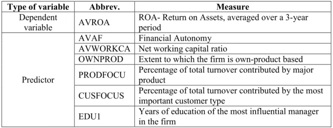
Based on skewness and kurtosis values, and aided by inspection of the frequency histograms with the normal distribution overlaid, we concluded there were seven variables whose transformation, any of the three, caused more harm than good, so the possibility of running MRA using such variables in a transformed version was discarded beforehand. As expected, these turned out to be the variables with a negative skew because the transformations considered were most adequate to correct positive skews (details available from Table 4).

Table 4 here.

For the remaining continuous variables (all positively skewed), both the milder SQRT transformation and the LOG10 transformation cured non-normality to a considerable extent though the transformation that worked best

(5)

International Journal of Research (IJR)

differed from variable to variable. Although some researchers have introduced distinct transformations into the same regression equation (e.g. Jordan, Lowe, and Taylor (1998)), this may seriously damage the external validity of the research. Therefore, we decided to build alternative datasets on which to run MRA: one in which the relevant variables („relevant‟ meaning all continuous variables except for those seven which would better remain as originally defined) were transformed with square root (dataset labelled „A2- SQRT transformation of relevant variables‟); and another one relying on logarithmic transformations (dataset „A3- LOG10 transformation of relevant variables‟). Either SQRT or LOG10 transformations require all variables to be positive. Thus, prior to performing any of these two transformations to obtain the two alternative datasets, we added a small constant (a „start‟) to the distribution of some variables so that the minimum value for all variables was just above zero (Fox, 1991; Tabachnik & Fidell, 2001).

The stages to follow in the data cleaning process were performed separately for each of the three datasets: (1) A1- No transformations performed; (2) A2- SQRT transformation of relevant variables; and (3) A3- LOG10 transformation of relevant variables.

3.2 Six Datasets Established from Adding Treatment of Univariate Outliers

The presence of outliers, that is, a certain value of a variable that by being extreme is inconsistent with the other values of that variable, inflates type I and type II errors and causes results to be sample-specific (Fox, 1991; Tabachnik & Fidell, 2001).

Firstly, we dealt with univariate outliers in the continuous variables. Given our sample size of 134 we considered univariate outliers would be those cells whose absolute standardised score exceeded 3.29 (p<0.001, two-tailed test) (Fox, 1991; Tabachnik & Fidell, 2001). The procedure of spotting and handling univariate outliers was performed on each of the three datasets created out of

normality considerations. Reflecting a salutary effect of variables transformation, there were fewer outliers in datasets A2 and (especially) A3 than were in dataset A1.

We administered two alternative procedures to eliminate the presence of univariate outliers:  Datasets „B1- Retention of univariate

outliers with alteration‟. To avoid throwing any information away and assuming that the univariate outliers were sampled from the target population and that the distribution of the variables in question in the actual population just happens to have more extreme values than a normal distribution (Tabachnik & Fidell, 2001), we considered keeping all the data while shrinking extreme scores to reduce their impact. This consisted of replacing each univariate outlier with a value just above/below the next maximum/minimum score on the respective variable that was a non-outlier. Far from seldom, new outliers were uncovered, so we carried this process on until no further outliers existed.

 Datasets „B2- Replacement of univariate outliers with the mean‟. Inspired by the possibility that outliers are not members of the target population we built additional datasets where univariate outliers were replaced with the mean value of the variable in question as computed only from non-outliers. Although this is a more prudent treatment than the one before, by replacing a cell with the mean value one is really depriving that cell of any information, thus a loss of information is inevitable.

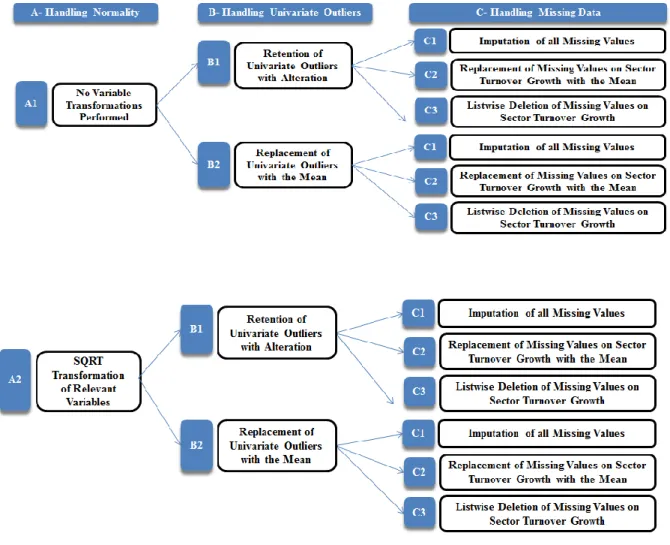
Figure 2 shows that to this point, we had already built six alternative datasets on which to repeat MRA, and two alternative datasets to estimate our structural equation model in LISREL because for this later it was unnecessary to consider variables transformation as explained earlier in section 3.1.

Figure 2 here.

Secondly, we worried about univariate outliers in dichotomous variables, as identified from very uneven splits in that scores for the

(6)

International Journal of Research (IJR)

cases in the small category are more influential than those in the category containing most of the cases (Tabachnik & Fidell, 2001). A further consequence of a very uneven split is that the correlations between such variables and others (either dichotomous or continuous) are truncated, thus, they are necessarily low even in the event that the corresponding population correlations are extremely high (Tabachnik & Fidell, 2001). Rummel (1970) suggests deleting dichotomous variables with 90-10 (and worse) splits between categories. All our dummy variables passed this „test‟.

3.3 Eighteen Datasets Established from Adding Treatment of Missing Data

There was only one variable where the issue of how best to handle missing data emerged: „CTURNGRW‟ (sector turnover growth). There were other four variables with missing data, but this was as few as 0.7 percent for each of them so it would not make much of a difference how it were handled (Tabachnik & Fidell, 2001).

Leaving missing data as missing and performing pairwise deletion was a possibility excluded beforehand. Reasons were twofold: (1) the likely lack of stability of the sample correlation matrix since each pair of correlations may be based on a different number and different subset of cases depending on the pattern of missing values (Tabachnik & Fidell, 2001); (2) in the LISREL programme of SEM the necessary asymptotic covariance matrix of correlations to cope with non-normality could only be estimated under listwise deletion (Jöreskog & Sörbom, 2002). PRELIS has implemented in it a convenient approach to increase listwise sample size, which can be used with ordinal/dichotomous or continuous variables, with any distribution, and does not require data are missing at random: this is the so-called „imputation of missing

values‟, which replaces missing observations

with real values obtained from cases with similar response pattern over a set of matching variables (variables with no missing values for any case) (Jöreskog & Sörbom, 2002). When there are several matching cases, the variance

ratio, defined as the quotient between the variance of the variable to impute for the matching cases to the total variance of that same variable for all cases without missing values, specifies the upper limit for imputation (Jöreskog & Sörbom, 2002). We used the default ceiling of 0.5, meaning the matching cases predict the missing values with a reliability of at least 1-0.5= 0.95 (Jöreskog & Sörbom, 2002).

In our study, the imputed variables were all variables with missing values and the matching variables were the remaining. All imputations were successful so final sample size under listwise deletion was 134. Furthermore, we were confident about those imputations, as all variance ratios were 0.000.

For the variable where missing data posed a problem, „CTURNGRW‟ (sector turnover growth), there were reasons for considering two further approaches:

 Datasets „C2- Replacement of missing values on CTURNGRW with the mean‟. This conservative procedure that allows the mean for the distribution as a whole to remain unchanged, offsets the criticism that imputation of missing values may be too liberal a procedure by involving guessing at missing data too much. The mean in question was the same mean computed to replace univariate outliers with the mean (datasets B2); it was not the mean calculated after having replaced univariate outliers with the mean because when doing so one would not be adding true information.  Datasets „C3- Listwise deletion of missing

values on CTURNGRW‟. This was inspired by the fact that listwise deletion is perhaps the most common approach to missing data across empirical performance research (e.g. Durand and Coeurderoy (2001); Hitt, Bierman, Shimizu, and Kochhar (2001)). Furthermore, Tabachnik and Fidell (2001) recommend repeating analyses under listwise deletion when some method of estimating missing values has been chosen; especially if sample size is small or the proportion of missing data is high.

In sum, we established three possible ways of dealing with missing data to each of the six

(7)

International Journal of Research (IJR)

datasets previously built, which boils down to eighteen datasets altogether, as shown in Figure 3, and numbered in Table 5 for convenience.

Figure 3 here. Table 5 here.

3.4 Latest Step Towards Getting Data Prepared for Analyses: Multivariate Outliers Considerations Leading to Further Nine Sub-datasets

Given that variables transformation and the handling of univariate outliers may result in a substantial decrease in the number of multivariate outliers (Tabachnik & Fidell, 2001), this was left to the latest stage of the data preparation process. Clearly enough, replacement of univariate outliers with the mean (datasets B2) exerted a strong salutary impact over multivariate outliers as compared with shrinkage of extreme scores (datasets B1), suggesting many of the univariate outliers were also multivariate outliers.

Multivariate outliers were sought separately for each of the eighteen datasets previously established by means of Mahalanobis tests performed jointly on the predictors and the dependent variables by running a regression in SPSS on an arbitrary variable (the case number). Degrees of freedom to evaluate the Mahalanobis distance were 26 (p-1)2 given the total 27 observed variables covered by our study (Tables 1 and 2). The chi-square table

2_{In theory given an infinite sample of the distribution of}

a known multivariate normal population (from which to assess the deviations of individual points) „p‟ is the number of predictors. However, where one uses the sample itself to estimate what is the base line from which any one point within the sample deviates, there is less genuinely independent information about what is a big deviation, so „p-1‟ should be more accurate than „p‟ and the result is that deviations within a finite sample are amplified to mean more than they seem to.

provides alternative p-values with which to evaluate Mahalanobis distances. A point with a probability of 0.01 should be acceptable in a sample of 100, since with a one percent chance of occurrence one would expect one such point and the rest of the sample should be able to absorb its effects. Thus, we were in search for points whose Mahalanobis distance was greater than 45.6417 (p<0.01).

Being aware that p<0.01 is certainly too tight for a sample size greater than 100, we resorted to the binomial test in order to analyse how many multivariate outliers would it be reasonable to expect for 134 cases and for 118 cases (where listwise deletion of missing data had been performed). The binomial tests progressed assuming the probability of success (i.e., of there being a multivariate outlier) was 0.01, so the probability of failure was 0.99. These tests indicated the appearance of zero, one, and two multivariate outliers were by far the most likely events, and their probabilities were quite close (when N=134, they were 26 percent, 35 percent, and 24 percent, respectively; when N=118, probabilities were 31 percent, 36 percent, and 22 percent, respectively).

Tabachnik and Fidell (2001) suggest multivariate outliers be deleted, or else they may distort the results in almost any direction. To the contrary, Cortina (2002) warns in most cases deletion increases the chances of supporting hypotheses, thereby being a dangerous procedure. Therefore, we decided to report the effect of deleting multivariate outliers only where there were more than two points whose Mahalanobis distance was too extreme (larger than 45.6417). For such datasets, we examined whether multivariate outliers were masking further multivariate outliers. This was not the case, that is, after having deleted the initially identified multivariate outliers there were either no further or a maximum of two more multivariate outliers.

Table 6 below indicates the datasets in which we repeated analyses having deleted multivariate oultiers.

(8)

International Journal of Research (IJR)

Dataset 3B could not be used to estimate the LISREL model because by trial and error we learned 118 was the minimum sample size, or else a warning message was provided that parameter estimates were not reliable. Considering for LISREL there was no need to try variables transformation, there were eight alternative datasets from which to estimate the LISREL model: datasets 1, 1B, 2, 2B, 3, 4, 5, and 6. For MRA there were eighteen alternative datasets plus nine sub-datasets as described in Table 5 and Table 6.

4. TRIANGULATION OF METHODS DESCRIBED

It has been acknowledged that theoretical concepts should better be measured indirectly from a number of questions (imperfect measures) that collectively reveal an unobservable (Priem & Butler, 2001). Factor scores, obtained from combining a number of observed variables that are linear functions of one or more constructs and a random error term, are more reliable than scores on individual observed variables because the „true measure‟ component of each variable will be added together whereas the „measurement error‟ components will be non-additive and random provided the pool of questions does justice to the multiple facets of the construct (Oppenheim, 1992; Tabachnik & Fidell, 2001). Given the advantages from employing multiple measures to operationalise theoretical constructs with measurement error removed, and given that for MRA performed on datasets 1 to 6 except 3B (i.e., the alternative datasets on which SEM in LISREL was estimated) there was the possibility to import into SPSS the multi-indicator factors‟ scores estimated in LISREL by means of confirmatory factor analysis, we considered using these in place of single observed variables. Scores from LISREL single-indicator factors were invariably ignored for MRA in SPSS, and the corresponding observed variable was used instead.

Although factor scores could also have been estimated in SPSS, the starting data for a factor analysis here is the Pearson correlation matrix, which assumes all variables are continuous; yet

our study comprised not only continuous but also dichotomous variables (as earlier addressed in section 2), whose essence is different and LISREL is able to handle them differently (Jöreskog & Sörbom, 2002). Although a dummy coding artificially lifts a nominal measurement level to a quantitative one where means and variances are calculated as with continuous variables, such calculations are clearly fake (Tacq, 1997). Just like ordinal variables, dichotomous variables lack an origin or unit of measurement and the only information available is counts of cases in each cell of contingency tables (Jöreskog & Sörbom, 2002). The single assumption behind an ordinal variable is that the subject that responds in a „higher‟ category has more of a certain characteristic than another one who responds in a „lower‟ category (Jöreskog & Sörbom, 2002). Given that all our dichotomous variables were coded in a way that „one‟ means the existence of the characteristic being measured and „zero‟ its absence (refer to Table 2), they are closer to the ordinal level of measurement than to the continuous one. Jöreskog and Sörbom (1993) argue estimates of polychoric and polyserial correlations should be computed to account for the different measurement levels of variables: continuous and ordinal. When ordinal variables are dichotomous, as in our study, PRELIS computes the matrix of tetrachoric and byserial correlations as a special case of the matrix of polychoric and polyserial correlations (Jöreskog & Sörbom, 2002).

Thus, for datasets 1 to 6 (except 3B), MRA was performed in two versions as regards the predictors‟ set: (1) multi-indicator LISREL factors‟ scores together with observed variables in place of the LISREL single-indicator factors; and (2) all predictors as observed variables. For this later version, selection of the observed variable to be used as a proxy for the multi-indicator factor is explained in Table 7.

Table 7 here.

All appropriate diagnostics were performed to every LISREL model as estimated from datasets 1 to 6 (except 3B), and to every regression equation as estimated from datasets

(9)

International Journal of Research (IJR)

1 to 18 including sub-datasets established from multivariate outliers deletion. For SEM we were mostly based on the appropriate fit indices, for MRA we concentrated on the analysis of residuals.

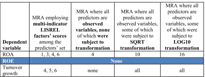
In MRA residuals are assumed to be normally distributed around the predicted values of the dependent variable (Cortina, 2002; Field, 2000; Fox, 1991; Tabachnik & Fidell, 2001; Tacq, 1997), and only upon the condition that errors are normal will OLS estimators be efficient (Fox, 1991). It followed the number of regression equations on which to base our postulates‟ evaluation was narrowed down considerably as we had to discard several datasets. Table 8 indicates the regression equations that based on the Shapiro-Wilk test of normality on the standardised residuals (corroborated by naked-eye tools such as the frequency histograms of standardised residuals with superimposed normal curves, and the expected normal probability plots) appeared in most senses to be accurate for the sample and generalizable to the population.

Table 8 here.

Table 8 shows the regression models where the dependent variable was profitability as measured by return on equity proved inadequate to make inferences about the population. It followed evaluation of the relationship between each predictor and ROE progressed solely based on classical hypothesis testing, and for purposes of MRA we were left with as few as two dependent variables: profitability as measured by return on assets, and turnover growth. Here results were generally well supported by the corresponding robustness analyses based upon sub-samples, as it was also the case for the LISREL model. Classical hypothesis testing was performed for each of the three dependent variables in turn, each one having been dichotomised in three alternative ways: just / 5% / 10% above average and just / 5% / 10% below average, respectively. Since we cleaned the data matrix for outliers, the average seemed to us more appropriate than the median to be used as the cut-off point to assign sample firms to „high‟

and „low‟ profitability/growth groups since, unlike the median, it captures the relevant information about all the observations. Variables tested included all observed predictors, as well as the four multi-indicator factors to inspect the incidence of measurement decisions. The underlying datasets ranged from 1 to 6.

5. EVIDENCE OF RESULTS VARIABILITY STEMMING FROM METHOD-RELATED OPTIONS

On estimating our LISREL model we decided to leave the default option of oblique factors, allowing them to covary with one another, as it offers theoretical advantages by representing reality more faithfully. Nevertheless, where we suspected factors to possibly be causing collinearity, we re-estimated the model while imposing orthogonalisation of the involved factors, thereby evaluating the stability of the sign and significance of the structural coefficients and interpreting the model free of (multi)collinearity bias. Oftentimes results diverged, and where this was the case we relied on results derived from orthogonalisation. In MRA, we looked at the difference between the full and the unique relationship of each predictor and the dependent variable; we also compared for each significant predictor its zero-order correlation with the dependent variable against its standardised regression coefficient (Beta) in terms of size and sign. Following the procedure described in the previous paragraphs, we learned that zero-order correlations even below 0.2 can introduce biases in the results.

For most of our postulates (14 out of 20, i.e., 70%), findings from MRA and classical hypothesis testing were mostly consistent between them and with those from LISREL, and they were invariant with dataset. However, noticeably enough, empirical evaluation of the remaining 30% of our postulates yielded remarkable inconsistencies. Indeed, for postulates 4, 8, 12, 13, 15, and 16, results differed according to the mix of data cleaning procedures ministered to the raw dataset,

(10)

International Journal of Research (IJR)

and/or method of analysis employed. Tables 9 to 14 are a friendly presentation of such empirical inconsistencies.

For the particular case of postulate 4 we speculate the inconsistent results from SEM, on the one hand, and MRA and classical hypothesis testing, on the other hand, as shown in Table 9, may be merely apparent. This is because upon re-estimation of the LISREL model by making the predictors „lackliq‟ (lack of liquidity) and „nodebt‟ (low leverage) orthogonal, significance previously (with oblique factors) found in every dataset, was lost for datasets 3 and 6. Given that „lackliq‟ is a variable with a number of large correlations with other predictors, we speculate that upon total orthogonalisation of „lackliq‟ with all those predictors with which it correlates, the path from „lackliq‟ to growth would invariably come out non-significant. However, we could not empirically confirm this conjecture due to convergence problems. Nevertheless, triangulation with MRA and classical hypothesis testing proved very useful in providing vivid evidence to our suspicion that liquidity management and growth are unrelated. This is because regardless of both the dataset used to run the regression and the operationalisation of the predictor by the observed variable „net working capital ratio‟ (AVWORKCA) or by a multi-indicator factor (lackliq), the respective regression coefficient was non-significant, consistently with the respective small zero-order correlations with the dependent variable. Furthermore, both the t-tests for „AVWORKCA‟ and the Wilcoxon tests for „lackliq‟ produced non-significance (p>0.1, two-tailed), regardless of both dataset employed and the operationalization of the grouping variable.

Table 9 here.

On assessing postulate 8, although the positive sign for the relationship emerged robustly (consistently with the sign for the corresponding zero-order correlation), ubiquity of significance could not be established since this proved sensitive to both method of analysis and the cleaning procedures ministered to the

raw dataset. Taking the evidence summarised in Table 10 altogether, we gathered the impression the positive relationship between sector growth and SMEs‟ growth was somewhat obliterated by guessing too much at data, either by replacing univariate outliers with arbitrary smaller scores for „CTURNGRW‟ and „TURNGROW‟, or by estimating missing data on „CTURNGRW‟ (as opposed to replacing it with the mean or, preferably, performing listwise deletion). Table 10 here.

Table 11 shows that only where a differentiation strategy was measured as a multi-indicator factor, there were instances of significance to support postulate 12: when differentiation was proxied by the observable „BRANPRIC‟ there was clearly a non-significant relationship, with the signs for the regression coefficients and correlations even oscillating between positive and negative; when differentiation was measured by the multi-indicator factor „differen‟, SEM indicated significance irrespective of dataset, and in MRA the regression coefficients were positive consistently with the zero-order correlations, and p<0.1 (two-tailed) in dataset 6. Both the chi-square tests for „BRANPRIC‟ and the Wilcoxon tests for „differen‟ were invariably associated with p>0.1 (two-tailed). Taking all these contradictory evidence, ubiquity of an effect or absence of it could not be established.

Table 11 here.

Although a negative relationship between a product focus strategy and profitability emerged quite robustly, t-values for postulate 13 oscillated between significance and non-significance depending on (1) dataset, (2) method of analysis employed, and (3) profitability measurement, with significance being notably boosted when profitability was measured by return on assets (Table 12). Instances of non-significance in SEM refer to datasets 4 and 5, which have in common that univariate outliers were replaced with the

(11)

International Journal of Research (IJR)

mean. On the other hand, MRA and Wilcoxon tests invariably indicated a non-significant (negative) relationship between a product focus strategy and profitability.

Table 12 here.

SEM in LISREL yielded consistency of the negative sign for the relationship underlying postulate 15, though significance proved sensitive to the mix of data cleaning procedures administered to the raw dataset and was boosted by measurement of profitability by ROE (Table 13). Yet, the zero-order correlation between „cusfocus‟ (customer focus strategy) and both ROA and ROE was small and, most importantly, positive. We suspected the misleading sign could be due to the significant positive correlation between „cusfocus‟ and turnover growth given that we specified non-correlated disturbances between profitability and growth. Our robustness analysis lent support to this conjecture: the emerging mean and median t-values for the path in question in the LISREL model estimated from different sub-samples for each dataset were invariably non-significant regardless of the operationalisation of profitability. Thus, triangulation of results proved of utmost importance to derive our conclusion that there is absence of a relationship between a customer focus strategy, at least as we measured it, and profitability. In fact, the regression coefficient of „CUSFOCUS‟ proved non-significant regardless of the version of MRA, consistently with the size of the zero-order correlations with ROA. Moreover, Wilcoxon tests indicated p>0.1 (two-tailed) regardless of both the operationalisation of profitability by ROA or ROE, and the underlying dataset.

Table 13 here.

Finally, although the positive sign for the relationship in postulate 16 was robustly inferred (consistently with the zero-order correlation between predictor and dependent variable), significance proved highly sensitive to statistical options (Table 14). Particularly, p<0.1 or p<0.05 (two-tailed) where univariate

outliers had been kept while reduced, whereas significance was not indicated by regressions where univariate outliers had been replaced with the mean, which could be due to the inherent loss of information. The mean rank of „CUSFOCUS‟ was higher for firms that exhibit superior growth, but significance in Wilcoxon tests was only achieved in a few instances, depending on the dataset and following the just aforementioned pattern.

Table 14 here.

6. CLOSING DISCUSSION

This paper is the result of an extensive work aimed at ascertaining the degree of incidence of data preparation, measurement decisions and method of analysis employed on the results, thereby creating an opportunity to evaluate robustness/sensitivity of each of the „findings‟. While preparation of data for analysis has frequently been an under-estimated issue, not even addressed by key papers, we show results of analyses may vary with alternative mixes of data cleaning procedures ministered to the raw dataset.

The Shapiro-Wilk test of normality on MRA standardised residuals where the dependent variable is ROA uncovered that retention of univariate outliers with shrinkage produces sample-specific results (Table 8). Indeed, where univariate outliers had been retained and reduced, the Shapiro-Wilk test was significant for all instances except where factors were part of the predictors‟ set and no multivariate outliers had been deleted; on the other hand, the assumption of normal residuals was met for all models where univariate outliers have been replaced with the mean. Likewise, where the dependent variable is growth, evidence was that generalizability of findings was boosted by replacing univariate outliers with the mean since where factor scores were used among the predictors‟ set in MRA, the assumption of normal residuals was met only if univariate outliers had been replaced with the mean (Table 8).

That retention of univariate outliers with reduction of extreme scores, unlike

(12)

International Journal of Research (IJR)

replacement of univariate outliers with the mean, may produce sample-specific results comes by no surprise because such treatment entails arbitrarily reducing outliers to a number just above/below the maximum/minimum non-outlier in the distribution. For example, the positive relationship between sector growth and SMEs‟ growth was somewhat obliterated by guessing too much at data, namely by replacing univariate outliers with arbitrary smaller scores for sector growth and SMEs‟ growth (postulate 8).

Furthermore, our study provides evidence to the salutary impact of taking a transformation of variables over the normality of residuals: when the dependent variable was growth and the observed variables were subject to any transformation (SQRT or LOG10) the assumption of normal residuals underlying MRA was met for all regressions run from any mix of data cleaning procedures (Table 8). To evaluate the degree of incidence exercised on the results by measurement decisions, we performed MRA in two versions as regards the predictors‟ set: (1) multi-indicator factors‟ scores estimated in LISREL through confirmatory factor analysis and imported into SPSS to be used as predictors together with observed variables in place of single-indicator factors; and (2) a single observed variable used in place of the multi-indicator factors, thus, all predictors being observed variables. Thereby we demonstrated that treating theoretical constructs as factors with several indicators may be advantageous over using a single variable. For example, the postulated relationship between a differentiation strategy and SMEs‟ growth (postulate 12) was more evident if the predictor was defined as a factor rather than proxied by a single observed variable. Secondly, the use of factors as predictors in MRA favoured residuals normality: where the dependent variable was ROA and where univariate outliers had been retained and reduced, the Shapiro-Wilk test was significant for all instances except where factors were part of the predictors‟ set (and no multivariate outliers had been deleted); furthermore, where the dependent variable was growth and factor

scores belonged in the predictors‟ set, the assumption of normal residuals was met if univariate outliers had been replaced with the mean; where the predictors‟ set comprised only observed variables the assumption was invariably broken.

While most theories and models in social sciences are formulated in terms of theoretical concepts not directly measurable (Jöreskog & Sörbom, 1993; Priem & Butler, 2001), perhaps the truth remains that testing in performance research usually relies on a single observed variable as a measure of a given construct. Implicit it is the huge assumption that such a variable, per se, represents the construct adequately, which becomes particularly dangerous since literature does not provide a pedigree to any particular measure of the variables hypothesised to be associated with performance. Not surprisingly, researchers have been using different single measures of the same constructs, which suggests data mining has prevailed (Titman & Wessels, 1988). Arguably, this is enough grounds to account for the many contradictory findings in empirical performance literature.

It follows method improvement in terms of measurement is well worth becoming a matter of increasing concern. For example, the constructs used in this study required the development of original measurement instruments. While considerable heed was taken to choose and to assess the psychometric properties of the instruments, and concerns over measurement difficulties were somewhat mitigated by mostly theoretically consistent results obtained in the study, researchers overall would better not underestimate the testing and validation of existing measurement instruments. In our study, relationships with profitability were differently recognisable from SEM in LISREL depending on whether this was operationalised by ROA or ROE. Furthermore, the regression models where the dependent variable was ROE proved inadequate to make inferences about the population.

On taking provisions to handle possible (multi)collinearity for both SEM and MRA, as earlier described, we learned that zero-order

(13)

International Journal of Research (IJR)

correlations even below 0.2 can introduce biases in the results. Consequently, one may cast doubt over findings derived from studies that overlooked the (multi)collinearity problem as most often collinearity is detected using the cut-off of 0.8 for the zero-order correlations between predictors; this „test‟ being passed most researchers do not worry any further about (multi)collinearity possibly biasing their findings.

While multi-method approaches are found in literature disappointingly sparsely, we believe it is high time multi-method studies became the norm. In fact, more than troublesome, our empirical evaluation of postulates 4 and 15 shows the use of different methods may prove very useful in clarifying the relationships between the predictors and the dependent variables.

We also concluded hypothesis testing not only lacks the elegance of SEM or even MRA, but also the power to find relationships. SEM in LISREL proved to be the statistical technique, or better said, collection of statistical techniques, with the greater power to find relationships. Furthermore, a key issue in favour of SEM is consideration of measurement error. An essential feature of the regression technique is that only the dependent variable is assumed to be subject to measurement error and other uncontrolled variation, while the predictors are assumed to be measured without error (Gujarati, 2003; Jöreskog & Sörbom, 1993; Tabachnik & Fidell, 2001; Tacq, 1997; Wonnacott & Wonnacott, 1990). Thus, in the likely event there is measurement error in the predictors, these and the error term will correlate which is a violation of the crucial assumption of classical linear regression analysis that the predictors must be uncorrelated with the random disturbance term. Consequently, estimates of both the intercept and the regression coefficients of the predictors with measurement error will be unreliable, biased and inconsistent; the variance of the disturbance will be incorrectly estimated as will the variance and standard errors of the regression coefficients; therefore, confidence intervals and hypothesis testing may provide misleading

conclusions about the significance of each predictor (Field, 2000; Gujarati, 2003; Jöreskog & Sörbom, 1993; Tabachnik & Fidell, 2001).

On the other hand, the measurement models in SEM include an error term for every observed variable that represents errors in the variables themselves (thus, random variables); they are usually interpreted as measurement errors, though they may also contain specific systematic components (Jöreskog & Sörbom, 1993; Williams, Edwards, & Vandenberg, 2003). Every error variance is estimated and removed from the analysis in the belief that such variance only confuses the picture of underlying processes; thus only common variance is left to analyse so as to obtain a theoretical solution uncontaminated by unique and error variability (Tabachnik & Fidell, 2001). Consequently, the structural coefficients in SEM are corrected for the measurement errors quantified in the measurement model (Cortina, 2002); the correlations among factors are free of measurement error (disattenuated correlations); and the reliability of measurement can be accounted for explicitly (Jöreskog & Sörbom, 1993; Ullman, 2001). Despite the particular setting of performance research underlying this paper, we believe to have sounded the bell as to how social sciences in general are likely to be populated with many underappreciated method problems and consequent misinterpretations of findings. Future research could confer the under-appreciated method issues their well-deserved importance for the sake of true progress in the different fields. Although we provided some hints on how best to handle normality, outliers, and missing data, future research is in demand to shed further light on what the best data cleaning procedures may be. So far, no hard-and-fast rules emerged and this has fostered discrepancy of results solely on account of discretionary decisions in these respects.

7. REFERENCES

Cortina, J. M. (2002). Big Things have Small Beginnings: an Assortment of "Minor"

(14)

International Journal of Research (IJR)

Methodological Misunderstandings.

Journal of Management, 28(3),

339-362.

Durand, R., & Coeurderoy, R. (2001). Age, Order of Entry, Strategic Orientation, and Organizational Performance.

Journal of Business Venturing, 16,

471-494.

Field, A. (2000). Discovering Statistics using

SPSS for Windows: Sage.

Fox, J. (1991). Regression Diagnostics: Sage. Gujarati, D. N. (2003). Basic Econometrics

(4th ed.): McGraw-Hill.

Hall, G., & Tu, C. (2004). Internationalisation and Size, Age and Profitability in the UK. In Dana L. P. (Ed.), The Handbook

of Research in International Entrepreneurship: Edward Elgar.

Hitt, M. A., Bierman, L., Shimizu, K., & Kochhar, R. (2001). Direct and Moderating Effects of Human Capital on Strategy and Performance in Professional Service Firms: A Resource-Based Perspective. Academy

of Management Journal, 44(1), 13-28.

Jordan, J., Lowe, J., & Taylor, P. (1998). Strategy and Financial Policy in U.K. Small Firms. Journal of Business

Finance & Accounting, 25(1&2), 1-27.

Jöreskog, K. G., & Sörbom, D. (1993). LISREL

8: Structural Equation Modelling with the SIMPLIS Command Language (5th

ed.): Scientific Software International, Inc.

Jöreskog, K. G., & Sörbom, D. (2002). PRELIS

2: User's Reference Guide (3rd ed.):

Scientific Software International, Inc. Lyon, D. W., Lumpkin, G. T., & Dess, G. G.

(2000). Enhancing Entrepreneurial Orientation Research: Operationalizing and Measuring a Key Strategic Decision Making Process. Journal of

Management, 26(5), 1055-1085.

Oppenheim, A. N. (1992). Questionnaire,

Design, Interviewing and Attitude

Measurement (New ed.). London, New

York: Continuum.

Priem, R. L., & Butler, J. E. (2001). Tautology in the Resource-Based View and the Implications of Externally Determined Resource Value: Further Comments.

The Academy of Management Review, 26(1), 57-66.

Robertson, C., & McCloskey, M. (2002).

Business Statistics- a Multimedia Guide to Concepts and Applications. Great

Britain: Arnold.

Rummel, R. J. (1970). Applied Factor

Analysis. Evanston: Northwestern University Press.

Scandura, T. A., & Williams, E. A. (2000). Research Methodology in Management: Current Practices, Trends and Implications for Future Research.

Academy of Management Journal, 43(6), 1248-1264.

Tabachnik, B. G., & Fidell, L. S. (2001). Using

Multivariate Statistics (4th ed.): Allyn

and Bacon.

Tacq, J. (1997). Multivariate Analysis

Techniques in Social Science Research- From Problem to Analysis: Sage.

Titman, S., & Wessels, R. (1988). The Determinants of Capital Structure Choice. The Journal of Finance, 43(1), 1-19.

Ullman, J. B. (2001). Structural Equation Modelling Using Multivariate Statistics (4th ed.): Allyn and Bacon.

Williams, L. J., Edwards, J. R., & Vandenberg, R. J. (2003). Recent Advances in Causal Modeling Methods for Organizational and Management Research. Journal of Management,

29(6), 903-936.

Wonnacott, T. H., & Wonnacott, R. J. (1990).

Introductory Statistics (5th ed.): John

(15)

International Journal of Research (IJR)

Table 1: Measures of the dependent variable ‘performance’ Dependent

Variable Abbrev. Definition Measure

Profitability

AVROE

ROE- Return on Equity, averaged over a 3-year period

Net profit Total Equity AVROA

ROA- Return on Assets, averaged over a 3-year period

Net Profit before Interest and Taxes Total Assets Growth TURNGROW Turnover growth- proportionate average over a 3-year period

Total Turnover= Net sales= Sales + Services Provided

Table 2: Measures of the independent variables Predictor

dimension Abbrev. Definition Measure

Capital Structure AVDER1 Gearing or Debt to Equity ratio (average over a 3-year period) Total Debt Total Equity AVAF Financial Autonomy (average over a 3-year period) Total Equity Total Assets

nodebt Low leverage or _{financial slack}

Theoretical construct derived from confirmatory factor analysis in Lisrel, loading positively on financial

autonomy and negatively on gearing

Liquidity Management LIQCRISI Whether the firm had experienced a severe liquidity

crisis over the previous 5 years

Open question

Dummy variable: 1= Yes; 0= No.

SUPHONE

Whether the firm frequently

pays suppliers late

“Using the scale in the card (provide laminated show card) please indicate the extent to which the following two situations have been occurring to your business over the past 5 years:

1. Pay suppliers only after having received their first telephone call claiming their credit;

2. Use early payment discounts offered by suppliers.” SUPDISC Whether the firm frequently uses early payment discounts

(16)

International Journal of Research (IJR)

0- Less than 10% of the times 1- 10-40% of the times 2- 41-60% of the times 3- 61-80% of the times

4- More than 80% of the times Dummy variables:

1 (if 2 or 3 or 4) = Frequently 0 (if 0 or 1) = Not Frequently. AVASTURN Assets turnover ratio (average over a 3-year period) Net Sales . Total Assets

AVWORKCA Net working _{capital ratio} Current Assets-Current Liabilities _{Total Assets}

lackliq Lack of liquidity / bad liquidity management

Theoretical construct derived from confirmatory factor analysis in Lisrel, loading positively on LIQCRISI and SUPHONE, and loading negatively on the remaining observed variables

Overall Cost Leadership (Competitive

Strategy)

OWNSTOR Whether the firm has its own stores

Dummy variable:

1= Yes (there is some percentage of sales assigned to own stores);

0= No (the firm does not have its own stores). BUDGET Whether the firm prepares budgets (i.e., costs and revenues forecasts, where net outcomes are

indicated) at least on a yearly basis Dummy variable: 1= Yes; 0= No. LOWCOST Importance attached to continuing, overriding concern for the lowest cost per

unit

“Imagine you have a handful of 100 points to assign among 3 aspects from the list I am presenting to you [8 options] according to the emphasis your business unit has placed in establishing its competitive posture over the past 5 years. How would you give out your points?”

Continuous variable measured on an interval scale.

MPLIST Whether the

(17)

International Journal of Research (IJR)

e-ISSN: 2348-6848, p- ISSN: 2348-795X Volume 2, Issue 05, May 2015 Available at http://internationaljournalofresearch.org extract a reliable and comput. list of stocks of raw materials at any time TRUEACC Whether the firm has a true cost accounting system in place

Dummy variable: 1= Yes; 0= No. (variable coded on the basis of a set of questions asked during interviews)

lowcost _leadershipLow cost

Theoretical construct derived from confirmatory factor analysis in Lisrel, loading negatively on OWNSTOR and positively on all other observable variables Differentiatio n Strategy PRODELAY Whether deliveries delays occur at least twice a year

“Using the scale on the card, please indicate how often is your production subject to delays as compared to the time they are due at the client.” (8 answer points)

Dummy variable: 1 (if 3 or more)= Yes; 0 (if 0, 1 or 2)= No. AVASTURN Assets turnover ratio (average over a 3-year period) Net Sales Total Assets

OWNPROD the firm is own-Extent to which product based

“Does this firm produce any products that are internally

conceived/developed and undergo no changes under specific customers‟ requirements? (Own-production or production to stock) What percentage of the total production do these products represent approximately?” 0-100%

Continuous and measured on an interval scale. BRANPRIC Whether brand name, product prestige, or firm reputation is important for the firm‟s pricing

“I would like to assess the extent to which a number of aspects contribute to your major product price level. Please tell me the number corresponding to your answer to each of the potential price determinants I am going to read out :

(18)

International Journal of Research (IJR)

Securing customer/long-term sales perspectives/financial health of customer;

Originality/creativity (other than through the production cost);

Brand name, product prestige, or firm reputation.”

Answer choices ranged from 0 (never / nothing at all) to 4 (always / very much)

Dummy variable: 1 (if 3 or 4) = Yes; 0 (if otherwise) = No.

PRODCERT Whether major product has a quality stamp on it

“Is your major product certified by any quality accredited standard? 0- No

1- Happening, not yet finished 2- Yes

3- Not applicable (either because (1)

the firm does not produce inside its premises, i.e., it outsources its

production; or (2) because no quality accreditation standards are available to the products of the firm)”

Dummy variable: 1 (if 1 or 2)= Yes; 0 (if otherwise) = No. BUDGET Same variable used for overall cost leadership

differen Differentiation leadership

Theoretical construct derived from confirmatory factor analysis in Lisrel, loading negatively on PRODELAY and AVASTURN, and positively on the remaining observable variables

Focus Strategy PRODFOCU Percentage of total turnover contributed by major product

Continuous and measured on an interval scale (0-100%) CUSFOCUS Percentage of total turnover contributed by the most important customer type

Continuous and measured on an interval scale (0-100%) Education (Human Resources) EDU1 Years of education of the most influential

Continuous variable measured on an interval scale.

(19)

International Journal of Research (IJR)

e-ISSN: 2348-6848, p- ISSN: 2348-795X Volume 2, Issue 05, May 2015 Available at http://internationaljournalofresearch.org manager in the firm Industry Performance (Market Conditions) CROE CROA CTURNGW

Variables are defined in the same way as the equivalent dependent variables at the firm level (Table 1), and used in turn. For example, CTURNGRW is not present for MRA where the dependent variable is profitability Size (control

Variable) ASSET01 Size of the firm Total balance sheet / Total assets Age (control

variable) AGEFIRM Age of the firm

Continuous measured on an interval scale: number of years from firm‟s birth/incorporation (rounded to the closest calendar year).

Figure 1: Basic LISREL structural equation model prior to estimation

EDU1 PRODFOCU OWNPROD BRANPRIC LOWCOST PRODCERT OWNSTOR CUSFOCUS SUPHONE SUPDISC PRODELAY TRUEACC BUDGET MPLIST LIQCRISI AVWORKCA AVASTURN AVAF AVDER1 CTURNGRW CROA CROE differen lowcost prodfocu cusfocus lackliq nodebt educatio growpot roepot roapot roa roe growth TURNGROW AVROA AVROE

(20)

International Journal of Research (IJR)

Table 3: Postulates developed Independent variable

Hypothesised sign for the relationship with SMEs’…

profitability growth

Degree of leverage + (P1) + (P2)

Effective liquidity

management + (P3) + (P4)

Years of formal education of

the most influential manager + (P5) + (P6)

Profitability of the industry in

which a SME operates + (P7) n.a.

Growth of the industry in

which a SME operates n.a. + (P8)

Pursuit of a low cost strategy - / none (P9) + (P10)

Pursuit of a differentiation

strategy + (P11) + (P12)

Pursuit of a product focus

strategy - (P13) + (P14)

Pursuit of a customer focus

strategy - (P15) + (P16)

SME size ? (P17- To be empirically

determined) No relationship (P18)

SME age ? (P19- To be empirically

determined) - (P20)

Table 4: Observed variables invariably kept in their original (non-transformed) version for MRA

Type of variable Abbrev. Measure

Dependent

variable AVROA

ROA- Return on Assets, averaged over a 3-year period

Predictor

AVAF Financial Autonomy AVWORKCA Net working capital ratio

OWNPROD Extent to which the firm is own-product based PRODFOCU Percentage of total turnover contributed by major _product CUSFOCUS Percentage of total turnover contributed by the most _{important customer type} EDU1 Years of education of the most influential manager