Big data model with SQL support for performance management in telecommunication networks

(1)

Universidade de Aveiro

Departamento de

Electr´

onica, Telecomunica¸

c˜

oes e Inform´

atica,

2014

Ricardo Jorge

de Santiago

Marques

Modelo de dados Big Data com suporte a SQL

para performance management em redes de

telecomunica¸

c˜

oes.

Big data model with SQL support for performance

management in telecommunication networks

(2)

(3)

Universidade de Aveiro

Departamento de

Electr´

onica, Telecomunica¸

c˜

oes e Inform´

atica,

2014

Ricardo Jorge

de Santiago

Marques

Modelo de dados Big Data com suporte a SQL

para performance management em redes de

telecomunica¸

c˜

oes

Disserta¸

c˜

ao apresentada `

a Universidade de Aveiro para cumprimento dos

requisitos necess´

arios `

a obten¸

c˜

ao do grau de Mestre em Sistemas de

Informa¸

c˜

ao, realizada sob a orienta¸

c˜

ao cient´ıfica do Doutor Jos´

e Luis

Guimar˜

aes Oliveira, Professor do Departamento de Electr´

onica,

Telecomu-nica¸

c˜

oes e Inform´

atica da Universidade de Aveiro. O trabalho descrito nesta

disserta¸

c˜

ao foi realizado na empresa Nokia Networks, sob a supervis˜

ao do

Mestre Carlos Filipe Marques Almeida, Engenheiro de Desenvolvimento de

Software da Nokia Networks.

(4)

(5)

Universidade de Aveiro

Departamento de

Electr´

onica, Telecomunica¸

c˜

oes e Inform´

atica,

2014

Ricardo Jorge

de Santiago

Marques

Big data model with SQL support for performance

management in telecommunication networks

Dissertation submitted to the University of Aveiro to fulfill the requirements

to obtain a Master’s degree in Information Systems, held under the

scien-tific guidance of Professor Jos´

e Luis Guimar˜

aes Oliveira, Department of

Electronics, Telecommunications and Computer Science from the

Univer-sity of Aveiro. The work described in this thesis was carried out in the

company Nokia Networks, under the supervision of Master Carlos Filipe

Marques Almeida, Software Development Engineer at Nokia Networks.

(6)

(7)

o j´

uri / the jury

presidente / president

Professor Doutor Joaquim Manuel Henriques de Sousa Pinto,

Pro-fessor Auxiliar, Universidade de Aveiro

vogais / examiners committee

Professor Doutor Jos´

e Luis Guimares Oliveira, Professor Associado,

Universidade de Aveiro

(Orientador)

Doutor(a) Rui Pedro Sanches de Castro Lopes, Professor

Co-ordenador, Instituto Polit´

ecnico de Bragana

(8)

(9)

Resumo

Com o tempo, a informa¸

c˜

ao mantida pelas aplica¸

c˜

oes tem vindo a crescer e

espera-se um crescimento exponencialmente na ´

area de banda larga m´

ovel

com o surgimento da LTE. Com este crescimento cada vez maior de dados

gerados, surge a necessidade de os manter por um per´ıodo maior de tempo e

as RDBMS n˜

ao respondem r´

apido o suficiente. Isto fez com que as empresas

se se tenham afastado das RDBMS e em busca de outras alternativas.

As novas abordagens para o aumento do processamento de dados

baseiam-se no debaseiam-sempenho, escalabilidade e robustez. O foco ´

e sempre o

processa-mento de grandes conjuntos de dados, tendo em mente que este conjunto

de dados vai crescer e vai ser sempre necess´

ario uma resposta r´

apida do

sistema.

Como a maioria das vezes as RDBMS j´

a fazem parte de um sistema

imple-mentado antes desta tendˆ

encia de crescimento de dados, ´

e necess´

ario ter

em mente que as novas abordagens tˆ

em que oferecer algumas solu¸

c˜

oes que

facilitem a convers˜

ao do sistema. E uma das solu¸

c˜

oes que ´

e necess´

ario ter

em mente ´

e como um sistema pode entender a semˆ

antica SQL.

(10)

(11)

Abstract

Over time, the information kept by the applications has been growing and

it is expected to grow exponantially in the Mobile Broadband area with the

emerging of the LTE. This increasing growth of generated data and the

need to keep it for a bigger period of time has been revealing that RDBMS

are no longer responding fast enough. This has been moving companies

away from the RDBMS and into other alternatives.

The new approaches for the increasing of data processing are based in the

performance, scalability and robustness. The focus is always processing

very large data sets, keeping in mind that this data sets will grow and it will

always be needed a fast response from the system.

Since most of the times the RDBMS are already part of a system

imple-mented before this trend of growing data, it is necessary to keep in mind

that the new approaches have to offer some solutions that facilitate the

conversion of the system. And one of the solutions that is necessary to

keep in mind is how a system can understand SQL semantic.

(12)

(13)

List of Figures

2.1 The big data 3Vs . . . .

4

2.2 The CAP Theorem . . . .

6

2.3 NoSQL database type Key-value store . . . .

7

2.4 Document database store

. . . .

8

2.5 Column family store . . . .

9

2.6 Graph database . . . .

10

2.7 Data stream cluster architecture

. . . .

11

2.8 Topology example

. . . .

12

2.9 Map Reduce framework architecture . . . .

13 2.10 Map Reduce execution diagram . . . .

14 2.11 Map Reduce example of rack awareness

. . . .

15 2.12 HDFS architecture . . . .

16 2.13 Data flows for map an shuffle joins[9] . . . .

23

3.1 High level of data flow and formats in streaming and storage clusters . . . . .

26

3.2 High-level structure of a Comma-separated values (CSV) file

. . . .

28

3.3 Topology implementation . . . .

28

3.4 Data stream cluster(all together) specifications . . . .

30

3.5 Data storage cluster with master/slave block files metadata . . . .

30

3.6 Data storage cluster(all together) specifications for storage scenario . . . .

31

3.7 Block size queries . . . .

32

3.8 Sequence file structure

. . . .

34

3.9 Record Columnar file (RCFile) structure [18] . . . .

34 3.10 Space used for different file formats with and without compression . . . .

36 3.11 Partitioning data and the improvement obtained . . . .

37 3.12 Hive Metadata schema . . . .

39 3.13 Data storage cluster(all together) specifications for queries scenario . . . .

43 3.14 Hive vs Shark in ne counter tables . . . .

44 3.15 Aggregation scenario with Hive and Shark . . . .

45

(16)

(17)

List of Tables

2.1 Hive Numeric Types[8] . . . .

18

2.2 Hive Data/Time Types[8] . . . .

18

2.3 Hive String Types[8] . . . .

19

2.4 Hive Misc Types[8] . . . .

19

2.5 Hive Complex Types[8]

. . . .

19

3.1 User Defined Functions (UDF) functions . . . .

42

3.2 Text files space used for a plan of 2 years

. . . .

47

3.3 Growth plan for text files space . . . .

48

3.4 RCFile with snappy compression space used . . . .

49

3.5 Growth plan for RCFile with snappy compression space . . . .

49

(18)

(19)

List of Acronyms

ASCII American Standard Code for Information Interchange

RDBM Relational Database Management System

ORM Object-relational mapping

JDBC Java Database Connectivity

ODBC Open Database Connectivity

XML EXtensible Markup Language

JSON JavaScript Object Notation

BSON Binary JavaScript Object Notation

CAP Consistency, Availability and Partition tolerance

ACID Atomicity, Consistency, Isolation, Durability

API Application Programming Interface

SQL Structured Query Language

GFS Google Distributed File System

HDFS Hadoop Distributed File System

DAG Directed Acyclic Graph

HQL Hive Query Language

CLI Command Line Interface

UDF User Defined Functions

UDAF User Defined Aggregate Function

MPP Massively Parallel Processing

RDD Resilient Distributed Datasets

PDE Partial DAG Execution

JVM Java Virtual Machine

NE Network Element

SAN Storage Area Network

RAC Real Application Clusters

KPI Key Performance Indicator

ETL Extract, Transform and Load

(20)

RCFile Record Columnar file

CSV Comma-separated values

JBOD Just a bunch of disks

(21)

Chapter 1

Introduction

1.1 Context

Over the years, internet has become a place where massive amount of data are generated

every day. This continuous growing of data and the need to organize and search it have

been revealing some lack of performance in the traditional Relational Database Management

System (RDBM) implemented so far.

RDBMs are massively used in the world, but the schema-rigidity and their performance

for big volumes of data, are becoming a bottleneck. The schema-rigid forces the correct design

of the model at the starting point of a project. However, if over time the data stream is a

volatile schema, the schema-rigidity can be a problem. If the structure of the data is changed,

this can force a migration of data from the RDBM, and possible data losses, at a great cost.

In terms of data volume, it is a more complex decision for an organization, especially if the

product is already implemented and needs to evolve. The knowledge acquired in the RDBMs

is very large and not only are the applications based on it, but also the mindset of people

that uses them. So, organizations are trying to reduce costs by shifting to other methods by

finding Structured Query Language (SQL) based systems to reduce the impact. RDBMs are

well integrated in the market and they are a very good, or even the best, solution for common

scenarios. However, for huge amount of data these systems can perform very poorly.

Changing the way on how to keep and interact with data is becoming more and more

frequent in the database world, not only because it is a trend in the IT world, but also

because now it is possible to save more data and for a longer period of time at a lower price.

With these possibilities, the organizations are exploring their data in a way that was not

possible a few years ago and can analyze, transform or predict future results based on the

amount of data kept. This type of possibilities can give organizations a greater leverage in

deciding for future strategies in the market.

For this amount of data, a catch-all term is used to identify it - Big Data. This term

defines data that exceed the processing capacities of conventional database systems. Big

data have become a viable cost-effective approach that can process the volume, velocity and

variability of massive data.

Telecommunication companies have infrastructures, with systems such as 2G, 3G or even

4G LTE, where the activity involved in the daily operations and future network planning

require data on which decisions are made. These data refer to the load carried by the network

and the grade of a service.

In order to produce these data, performance measurements

(22)

are executed in the Network Elements (NEs), collecting data that is then transferred to

an external system, e.g.

a Monitoring System, for further evaluation.

In a 2G and 3G

system, the size of data generated by the NEs is considerable, but sustainable. With the

introduction of 4G LTE systems, and anticipating the future 5G systems, the data growth

has been exponential, making storage space and RDBMs performance a problem. Facing

this problem, telecommunication companies have turned to Big Data systems trying to find

alternatives for the data growth.

1.2 Objectives

Facing the increase of data to store and process, it is necessary to analyze solutions that

allow, in a viable and cost-effective way, to process, store and analyze it. For this work,

some of the solutions used in Big Data systems were studied. Different solutions to store and

analyze the data were studied. The key objectives are namely:

• studying different technologies/frameworks, taking into consideration the support to

SQL and its scalability.

• evaluating the data load from the NEs.

• evaluating storage solutions.

• evaluating SQL support and performance over a typical scenario.

• defining specifications of a Big Data system and resources needed.

1.3 Structure of the document

This document is structured in 3 chapters:

• Big data ecosystem - in this chapter are described several types of systems and different

practices used on each system.

• Evaluation scenario - in this chapter, a test environment is specified and the results of

each evaluation are presented.

• Conclusion and future work - in this chapter is summarized some conclusions and also

point out possible future work.

(23)

Chapter 2

Big data ecosystem

2.1 Introduction

The term big data has been used to describe data that exceed the processing capacities of

conventional database systems. In these data lie valuable patterns and hidden information,

which can be analyzed to create valuable information to an organization. The analytics can

reveal insights previously hidden due to the cost to process, being only possible by exploration

and experimentation.

Most of the organizations have their data in multiple applications and different formats.

The data can be collected by smart phones, social networks, web server logs, traffic flow

sensors, satellite imagery, broadcast audio streams, banking transactions, MP3s music, Global

Positioning System (GPS) trails and so on. These types of collected data contain structured

and unstructured data that can be analyzed, explored and experimented for patterns.

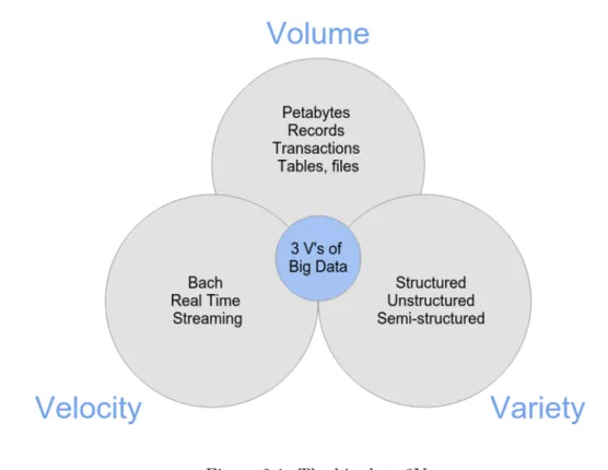
There are some aspects that need to be characterized to better understand and clarify the

nature of Big Data. These aspects have been identified as the three Vs - Variety, Velocity

and Volume (figure 2.1) [1] [2].

Volume

This is one of the main attractions of big data. The ability to process large amounts of

information that, in conventional relational databases infrastructures, could not be handled[1].

It is common to reach Terabytes and Petabytes in the storage system and sometimes the same

data is re-evaluated with multiple angles searching for more value in the data. The options to

process the large amounts of data are parallel processing architectures such as data warehouses

or databases, for instance Greenplum, or platform distributed computing system - Apache

Hadoop based solutions[2]. This choice can be mostly defined by the Variety of the data.

Velocity

With the growth of social media, the way we see information has changed. There was a

time when data with some hours or days were considered recent. Organizations have changed

their definition of recent and have been moving towards the near real-time applications.

The terminology for such fast-moving data tends to either streaming data, or complex event

processing[2].

(24)

Figure 2.1: The big data 3Vs

Streaming processing has two main reasons to be considered. One main reason is when

the input data are too fast to be entirely stored and need to be analyzed as the data stream

flows[1]. The second main reason is when the application sends immediate response to the

data - mobile applications or on line gaming, for example[1]. However, velocity is not only for

the data input but also for the output - as the near real-time systems previously mentioned.

This need for speed has driven developers to find new alternatives in databases, being part

of an umbrella category known as NoSQL.

Variety

In a Big Data system it is common to gather data from sources with diverse types. These

data does not always fit the common relational structures, since it may be text, image data,

or raw feed directly from a sensor. Data are messy and the applications can not deal easily

with all the types of data. One of the main reasons for the use of Big Data systems is the

variety of data and processes to analyze unstructured data, and be able to extract an ordered

meaning of it[2].

In common applications, the process of moving data from sources to a structured process

to be interpreted by an application may imply data loss. Throwing data away can mean the

loss of valuable information, and if the source is lost there is no turning back.“This underlines

a principle of Big Data: when you can, keep it ”[2].

Since data sources are diverse, relational databases and their static schemas nature have

a big disadvantage. To create ordered meaning of unstructured or semi-structured data, it is

necessary to have a system that can evolve along the way, following the detection and

extrac-tion of more valuable meaning of the data over time. To guaranty this type of flexibility, it is

(25)

necessary to encounter a solution on how to allow organization of data but without requiring

an exact schema of data before storing, the NoSQL databases meet these requirements.

2.2 NoSQL

NoSQL is a term that was originated in a meet-up focused on the new developments

made in BigTable, by Google, and Dynamo, by Amazon, and all projects that they inspired.

However, the term NoSQL caught out like wildfire and up to now, it is used to define databases

that do not use SQL. Some have implemented their query languages, but none fit in the notion

of standard SQL. An important characteristic of a NoSQL database is that it is generally

open-source, even if sometimes the term is applied to closed-source projects.

The NoSQL phenomenon has emerged from the fact that databases have to run on

clusters[3]. This has an effect on their data model as well as their approach to consistency.

Using a database in a cluster environment clashes with the Atomicity, Consistency, Isolation,

Durability (ACID) transactions used in the relational databases. So NoSQL databases offer

some solutions for consistency and distribution. However, not all NoSQL databases are

fo-cused on running in clusters. The Graph databases are similar to relational databases, but

offer a different model focused on data with complex relationships.

When dealing with unstructured data, the NoSQL databases offer a schemeless approach,

which allows to freely adding more records without the need to define or change the structure

of data. This can offer an improvement in the productivity of an application development by

using a more convenient data interaction style.

The ACID transactions are well known in relational databases. An ACID transaction

allows the update of any rows on any tables in a single transaction giving atomicity. This

operation can only succeeds or fails entirely, and concurrent operations are isolated from each

other so they cannot see a particular update.

In NoSQL databases, it is often said that they sacrifice consistency and do not support

ACID transactions. Aggregate-oriented databases have the approach of atomic manipulation

in a single aggregate at a time, meaning that to manipulate multiple aggregates in an atomic

way it is necessary to add application code. Graph and aggregate-ignorant database usually

support ACID transactions in a similar way to relational database.

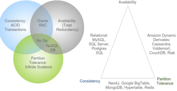
In NoSQL it is always common the reference to the Consistency, Availability and Partition

tolerance (CAP) Theorem. This theorem was proposed by Eric Brewer(may also be known

as Brewer’s Conjecture) and proven by Seth Gilbert and Nancy Lynch[3]. CAP are the tree

properties of the theorem and represent:

· Consistency - all nodes see the same data at the same time.

· Availability - a guarantee that every request receives a response about whether it was

successful or has failed.

· Partition tolerance - the system continues to operate despite arbitrary message loss or

failure from part of the system.

However, the CAP theorem defines that in a distributed system a database can only offer

two out of the three properties (figure 2.2). In other words, you can create a system that is

(26)

consistent and partition tolerant, a system that is available and partition tolerant or a system

that is consistent and available, but not all the three properties[3].

Figure 2.2: The CAP Theorem

As seen, the CAP Theorem is very important on the decision of which distributed system

to use. Based on the requirements of the system it is necessary to understand which property

is possible to give up. The distributed databases must be partition tolerant, so that the

choice is always between availability and consistency, if the choice is availability there is the

possibility of eventual consistency. In eventual consistency the node is always available to

requests but, the data modification is propagated in the background to other nodes. At any

time the system may be inconsistent, but the data are still accurate.

NoSQL Database Types

For a better understanding of NoSQL data stores, it is necessary to compare their features

with RDBMs, understand what is missing and what is the impact in the application

archi-tecture. In the next sections it will be discussed the consistency, transactions, query features,

structure of the data, and scaling for each type presented.

Key-Value

Key-value database are the simplest NoSQL data stores based on a simple hash table. In

this type of data stores it is the responsibility of the application to know which type of data

is added. The application manages the key and the value without the key-value store caring

or knowing what is inside(figure 2.3). This type of data stores always use primary-key access

which gives a great performance and scalability.

In key-value database, the consistency is only applicable in a single key because the only

operations are ’get’, ’put’ or ’delete’ a single key. There is the possibility of an optimistic

write, but the implementation would be expensive, because of the validation of changes in

(27)

Figure 2.3: NoSQL database type Key-value store

the value from the data store. The data can be replicated in several nodes and the reads are

managed by the validation of the most updated writes.

For transactions, the key-value database has different specifications and, in general, there

is no guarantee on the writes. One of the concepts is the use of quorums.

1

The query is by key and quering by value is not supported. For searching by value, it is

necessary that the application reads the value and process it itself. This type of database,

usually, does not give a list of keys, so it is necessary to give a thought about the pattern/key

to use on key-value database[3].

The structure of data for key-value database is irrelevant, the value can be a blob, text,

JavaScript Object Notation (JSON), EXtensible Markup Language (XML) or any other

type[3]. So, it is the responsibility of the application to know what type of data is in the

value.

If there is the need for scaling, the key-value stores can scale by using sharding

2

. The

sharding for each node could be determined by the value of the key, but it could introduce

some problems. If one of the nodes goes down, it could implye data loss or unavailable and

no new writes would be done for keys defined in sharding for that node.

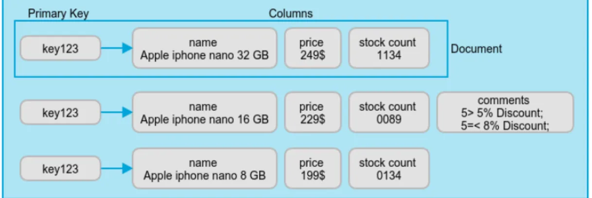
Document

Document databases stores documents in the value part of the key-value store, where the

value is examinable (figure 2.4). The type of files can be XML, JSON, Binary JavaScript

Object Notation (BSON) and many more self-described type of files[3]. The data schema can

differ across documents and belong to the same collection without a rigid schema such as in

RDBMs. In documents, if a given attribute is not found, it is assumed that it was not set or

relevant, but it can create new attributes without the need to define it or change the existing

ones.

Some document databases allow configuration of replica sets choosing to wait for the

writes in a number of slaves or all. In this case all the writes need to be propagated before it

returns success allowing consistency of data but affecting the performance.

The traditional transactions are generally not available in NoSQL solutions. In document

1_{Write quorum is expressed as W>N/2, meaning the number of nodes participating in the write (W).}

Must be more than a half the number of nodes involved in replication (N)[3].

(28)

Figure 2.4: Document database store

databases, the transactions are made at single-document level and called ’atomic transactions’.

Transactions involving more than one operation are not supported.

To improve availability in document databases, it can be done by replicating data using

master-slave setup[3]. This type of setup allows access to data, even if the primary node

is down, because data is available in multiple nodes. Some document databases use replica

sets where two or more nodes participate in an asynchronous master-slave replication. All the

requests go through the master node, but if the master goes down, the remaining nodes in the

replica set vote among themselves to elect the new master. The new requests will go through

the new master and the slaves will start receiving data from the new master. If the node that

failed gets back online, it will join the list of slaves and catch up with other nodes to get the

latest information. It is also possible to scale, for example, to archive heavy-reads. It would

be a horizontal scaling by adding more read slaves, the addition of nodes can be performed

during time the read load increases. The addition of nodes can be performed without the need

of application downtime, because of the synchronization made by the slaves in the replica set.

One of the advantages of document databases, when compared to key-value databases,

is that we can query the data inside the value. With the feature of querying inside the

document, the document databases get closer to the RDBMs query model. The document

databases could be closer to the RDBMs, but the query language is not SQL, some use query

expressed via JSON to search the database.

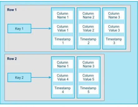
Column-Family

Column-family databases allow storing data in a key-value type and the values are grouped

in multiple column families. Data in column-family databases is stored in rows with many

columns associated to a key. The common data stored in column-family database are groups

of related data that are usually accessed together as shown in figure 2.5.

In some column-family databases, the column consists of a name-value pair where the

name behaves as key for searches. The key-value pair is a single column and, when stored,

it receives a timestamp for data control. It will allow the management of data expiration,

resolve data conflicts, stale data, among others[3]. In RDBMs, the key identifies the row and

the row consists in multiple columns. The column-family databases have the same principle,

but the rows can have different columns during time, without the need to add the columns to

(29)

Figure 2.5: Column family store

other rows. In column-family databases there are other type of columns, the super columns.

The super columns can be defined as a container of columns being a map to other columns;

this is particulary good when the relation of data needs to be established.

Some column-families use quorums to eventually achieve consistency, but their focus are

on availability and partition tolerance. Others guaranty consistency and partition tolerance,

but lack in availability.

Transactions in column-family databases are not made in the common sense, meaning

that it is not possible to have multiple writes and decide if we want to commit or roll-back

the changes. In some column-family databases the writes are made in an atomic way, being

only possible to write at the row level and will either succeed or fail.

As previously mentioned, the availability in column-family database relies on the choice of

the vendor. To improve the availability some column-family databases use quorums formulas

to improve availability. The availability improvement in a cluster will decrease the consistency

of data.

The design of column-family databases is very important, because the query features for

this type of databases is very poor. In this type of databases it is very important to optimize

the columns and column families for the data access.

The scaling process depends on the vendor. Some offer a solution to scale with no single

point of failure, presenting a solution with no master node, and by adding more nodes, it

will improve the cluster capacity and availability. Others offer consistency and capacity by a

master node and RegionServers. By adding more nodes, it will improve the capacity of the

cluster keeping the data consistent.

(30)

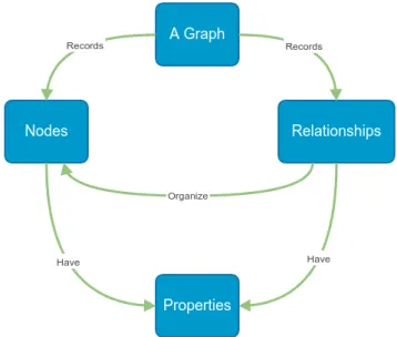
Graph

Graph databases allow the representation of relationships between entities. Entities, also

known as nodes, contain entity properties and they are similar to an object instance in

applications. The relationships are known as edges and contain properties and direction

significance, as figure 2.6 shows.

Figure 2.6: Graph database

The graph databases allow relationships as in RDBMs, but if there is a change in a

relationship the scheme change will not be necessary. One of the key features of this type

of database is the fast traversing of the joins or relationships, and that the relations are not

calculated at query time - they are persisted as a relationship. Relationships are first-class

citizens and not only have types, but can also have start node, end node, and properties of

their own allowing to add intelligence to the relationships[3].

One of the key features of graph databases is the relationships and, therefore, they operate

on connected nodes. Because of this type of feature, most graph databases do not support

the distribution of nodes on different servers. Graph databases ensure consistency and

trans-actions, but in some vendors they can also be fully ACID compliant. The start or end node

does not need to exist and it can only be deleted if no relationship exists.

As previously said, the graph databases can ensure transactions, but it is necessary to

keep in mind that the workflow of the transactions can differ from vendor to vendor. So,

even in this, there are some characteristics similar to RDBMs. The standard way of RDBMs

managing transactions can not be applied to graph databases.

For availability, some vendors offer the solution of replication on nodes to increase the

availability on reads and writes. This solution implies a master and slaves to manage

repli-cation and management of data. Other vendors provide distributed storage of the nodes.

Querying a graph database requires a domain-specific language for traversing graphs.

Graphs are really powerful on traversing at any depth of the graph and, the node search can

be improved with the creation of indexes.

(31)

Since graph databases are relation oriented, it is difficult to scale them by sharding, but

some techniques are used for this type of databases. When the data can entirely fit in RAM,

this will give a better performance for the database and for traversing the nodes throw the

cluster. Some techniques go through adding slaves, with read-only access, to the data or,

through all the writes passing on the master. This pattern is defined by writing once and

reading from many. However, it can be applied when the data is large enough to fit in RAM

but small enough to be replicated. The sharding technique is only used when the data is too

big for replication.

2.3 Streaming data

With the size of data that modern environments deal with, it is required a processing

computation on streaming data. To process the data and transform it to the defined structure,

it is necessary a distributed real-time computation system which will deal with the data

stream. The system must scale and perform Extract, Transform and Load (ETL) over a big

data stream.

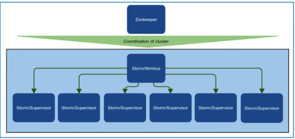
Storm

Storm is a real-time distributed computation system and it is focused in scalability,

re-silience (fault-tolerance), extensible, efficient and easy to administer[4]. Storm uses a

Nim-bus/Supervisors architecture, which is the same definition of master and slaves:

• Nimbus daemon - this is the master node and it is responsible for assigning tasks to the

worker nodes, monitoring cluster failures and deploy the topologies (the code developed)

around the clusters.

• Supervisors daemon - this is the worker node and listens for work assigned by the

Nimbus. Each worker executes a subset of a topology.

Storm uses Zookeeper to coordinate between Nimbus and Supervisors, as represented in

figure 2.7, and their state is hold on disk or in Zookeeper.

(32)

Zookeeper, a project inside the Hadoop ecosystem (section 2.4), is a centralized service

used for maintaining configuration information, naming, providing distributed

synchroniza-tion, and providing group service. The main focus is to enable highly reliable distributed

coordination.

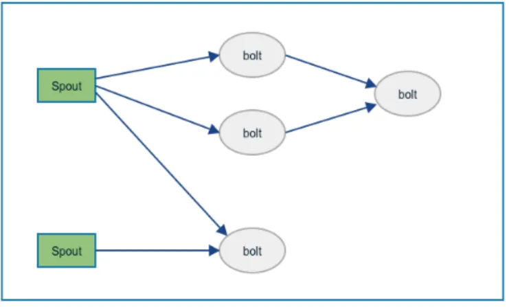
By using Storm, tuples containing objects of any type, can be manipulated and

trans-formed. Storm uses three abstractions (figure 2.8):

• spout - is the source of streams in computations and typically reads from queuing

brokers.

• bolt - most of the logic of a computation goes into bolts, and bolts processes input,

from the streams, and produces a number of new outputs.

• topology - is the definition of the network made of spouts and bolts, and can run

indefinitely when deployed.

Figure 2.8: Topology example

Storm offers the flexibility to execute ETL and the connection with several sources, such as,

a real-time system or a off-line reporting system using common RDBMs or Hadoop Distributed

File System (HDFS).

2.4 Storage

Hadoop

Google Distributed File System (GFS) and the Map-Reduce programming model have

had enormous impact in parallel computation. Doug Cutting and Mike Cafarella started to

build a framework called Hadoop based on GFS and Map-Reduce papers. The framework is

mostly known by the HDFS and the Map-Reduce features, and it is used to run applications

on large clusters of commodity hardware.

Map-Reduce

Communities, such as the High Performance Computing (HPC) and Grid Computing,

have been doing large-scale data processing for years. The large-scale data processing was

(33)

done by APIs like Message Passing Interface (MPI), and the approach was to distribute work

across clusters of machines, which access a shared file system, hosted by a Storage Area

Network (SAN). This type of approach works only for computer-intensive jobs. When there

is the need to access large data volume the network bandwidth is a bottleneck and compute

nodes become idle.

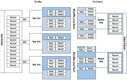
The Map-Reduce breaks the processing into two phases, the map phase and the reduce

phase. The map function is processed by the Map-Reduce framework before being sent to

the reduce function, and each phase has a key-value pair as input and output (figure 2.9)[5].

Figure 2.9: Map Reduce framework architecture

This functions and key-value structures are defined by the programmer, and the processing

sorts and groups the key-value pairs by key. The framework can detect failure for each phase

and, detecting the failure on map or reduce tasks, it will reschedules the jobs on healthier

machines. This type of reschedule can be performed because Map-Reduce is a share-noting

architecture, meaning that the tasks have no dependencies on one another[5].

A Map-Reduce job is a unit of work that we want to be performed over a set of data, and

run by dividing it into tasks of map and reduce. All the jobs are coordinated by a jobtracker,

and it will schedule tasks to run on tasktrackers. The function of a trasktracker is to run a

task and send progress reports to the jobtracker, while the jobtracker keeps a record of the

overall progress of each job. Since the tasks can fail, the jobtracker can reschedule it on a

different tasktracker.

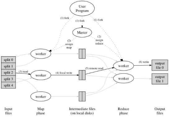
As seen in the description of the workflow (figure 2.10) Map-Reduce has a master and

slaves which collaborate on getting the work done. The definition of master and slave is made

by the configuration file and therefore, they can know about each other. The master has an

algorithm on how to assign the next portion of the workfigure[5]. This division is called ’split’,

and it is controlled by the programmer. By default, the input file is split into chunks of about

64 MB in size, preserving the complete lines of the input file. The data resides in HDFS,

(34)

which is unlimited and linearly scalable. So, it can grow by adding new servers as needed.

This type of scalability solves the problems of central file server with limited capacity.

Figure 2.10: Map Reduce execution diagram

The Map-Reduce framework never updates the data. It writes a new output, avoiding

update lockups. Moreover, to avoid multiple process writing in the same file, each reducer

writes its own output to the HDFS directory designated for the job. Each reducer has its

own ID, and the output file is named using that ID to avoid any problem with input or

output files in the directory. The map task should run in nodes where the HDFS data is,

to improve optimization - called data locality optimization, because it does not use cluster

bandwidth[5]. The Map output is written to the disk, since it is an intermediate output and

it can be discarded when the job from the reducer is complete.

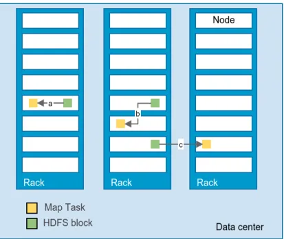
Sometimes, when looking for a map slot on a node inside the rack, it is necessary to

schedule the task outside the rack.

An off-rack node is used, which results in an

inter-rack network transfer[5]. This is only possible, because Map-Reduce is inter-rack-aware, it knows

where the data and tasktracker are over IP (figure 2.11). This awareness allows assigning

computation to the server that has data locally. If this is not possible the Map-Reduce will

try to select the server closest to the data, reducing the number of hops in the network traffic.

Hadoop Distributed Filesystem

Over the years data have grown to the point of being too big to store in a single physical

machine. This created the necessity to partition data across several machines and filesystems

that manage storage across a network of machines - distributed filesystems.

These type

(35)

Figure 2.11: Map Reduce example of rack awareness

of filesystems are network-based and more complex than normal filesystems. They create

challenges such as tolerance to node failure without suffering data loss. Creating a distributed

filesystem over server machines can be costly. Therefore, it is necessary to reduce costs by

using commodity hardware.

Hadoop comes with a distributed filesystem called HDFS based on GFS, and it is

de-signed to store very large files with streaming data access patterns. Large files mean files

with hundreds of megabytes, gigabytes, or terabytes in size(some clusters today are

stor-ing petabytes). Streamstor-ing data access in HDFS is based on the data processstor-ing pattern

write-once, read-many-times[6]. Since the reading is very important, the dataset generated

or copied from source is analyzed many times and it will involve a large portion, if not all,

of it making very important the time to read all the dataset. HDFS does not need highly

reliable hardware to run, since it is design to run on clusters of commodity hardware. Even

if a node fails, HDFS is designed to carry on working without interruption.

There are some problems where HDFS does not work so well. When low-latency

access-ing data is required, HDFS will not work well because it is optimized for deliveraccess-ing a high

throughput of data. The limit to the number of files in a filesystem is governed by the amount

of memory in the master. So, if an application generates a big amount of small files HDFS

may not be the best fit. The HDFS writes are made at the end of the file, and there is no

support for multiple writers, or modifications at arbitrary offset in the file[6]. So, if an

ap-plication needs to perform multiple writes or arbitrary files modification, HDFS it is not the

best solution. The information of each file, directory, and block is stored in memory taking

about 150 bytes, which can be possible for millions of files but not for billions because of the

limits of current hardware.

As previously mentioned, HDFS cluster consists of one master node and many worker

nodes. The master is named of Name Node and workers are named of Data Node (figure 2.12).

(36)

The Data Nodes are the ones that store the data, and the Name Node is in charge of file

system operations. Without the Name Node the cluster will be inoperable, and no one can

read or write data.

Figure 2.12: HDFS architecture

Since commodity servers will fail, a solution to keep the data resilient is to maintain

multi-ple copies of data across nodes. Keeping several copies, even if a node fails, will maintain data

accessible and the system on-line. Data Node store the data, retrieve blocks, and periodically

report a list of blocks that they store to the Name Node. The Name Node is a Single Point

of Failure, and if it fails, all the files on the filesystem would be lost, and there would be

no way of knowing how to reconstruct the files stored in the Data Nodes. For this problem,

HDFS provides two mechanisms to keep it resilient to failure. One of the mechanism, is to

back up the files that make a persistent state of the filesystem. It can be configured to write,

synchronously and atomically, its persistent state to multiple filesystems. The second

mecha-nism, is to run a secondary Name Node. This secondary Name Node only merges periodically

the namespace image with the edit log, preventing the edit log from becoming too large. This

Name Node has the same hardware characteristics as the primary, and it will be ready for

use in case of the fail from the primary.

2.5 Querying Big Data

Hadoop ecosystem solves the cost-effective problem of working with a large data set. It

introduces a programming model and a distributed file system, splitting work and data over a

cluster of commodity nodes. The Hadoop ecosystem can scale horizontally, making it possible

to create bigger data set over time. However the challenge is, how to query all the data from

the sources available?

A challenge for companies using, or planning to use, Big Data systems is how to query their

data on several infrastructures. The number of users knowing SQL is large, and applications

were developed using this knowledge. So, there is a necessity to migrate to Big Data systems

with the smaller impact in applications, becoming very important to use query engines that

can query on Big Data systems, and with characteristics of being SQL like. This would reduce

the cost in a company, using the knowledge already achieved by SQL users, and the time to

learn new methods or languages would be unnecessary. The migration of applications would

be minimum, creating the possibility to companies to be in the market with new features and

(37)

a new infrastructure.

2.5.1 HIVE

Hive was created by the Facebook Data Infrastruture Team in January 2007 and available

as open source in August 2008. The main reason for the development of Hive was because

of the difficulty of end users on using map-reduce jobs in Hadoop, since it was not such an

expressive language as SQL, and it brought that data closer to the users[7]. In Facebook,

Hive is used from simple summarization jobs to business intelligence, machine learning and

product features. Hive structures data into database concepts like tables, columns, rows, and

partitions, but it is possible for users to extend to other types and functions[7].

Hive is separated in some components, each one with a responsibility. In terms of system

architecture, Hive is composed by:

• Metastore - this component stores the system catalog and metadata of the tables,

partitions, columns and types, and more. To interact with this information Hive uses

a thrift interface to connect to an RDBM using a Object-relational mapping (ORM)

(DataNucleus) to convert object representation into relational schema and vice versa.

This is a critical component for Hive and, without it, it will not be possible to execute

any query on HDFS. So, for safety measures, it is advised to keep a regular back up of

the Metastore or a replicated server to provide the necessary availability for a production

environment.

• Driver - this component manages the lifecycle of Hive Query Language (HQL)

state-ments, maintains the session handle and any session statistics.

• Query Compiler - this component is responsible for the compilation of HQL

state-ments to the Directed Acyclic Graph (DAG) of map-reduce jobs. The metadata in the

Metastore is used to generate the execution plan and processes HQL statements in four

steps:

– Parse - uses Antlr to generate an abstract syntax tree for the query

– Type checking and Semantic Analysis - in this step, the data from the Metastore

is used to build a logical plan and check the compatibilities in expressions flagging

semantic errors.

– Optimization - this step consists of a chain of transformations such that the

oper-ator DAG is passed as input to the next transformation. The normal

transforma-tions made are column pruning, predicate pushdown, partition pruning and map

side joins.

– Generation of the physical plan - after the optimization step, the logical plan is

split into multiple map-reduce and HDFS tasks.

• Execution Engine - this component executes the tasks generated by the Query

Com-piler in the order of their dependencies. The executions are made using Hadoop and

Map-Reduce jobs, and the final results are stored in a temporary location and returned

at the end of the execution plan ends.

(38)

• Hive Server - this component provides a thrift interface and Java Database

Connectiv-ity (JDBC)/Open Database ConnectivConnectiv-ity (ODBC) server, allowing external applications

to integrate with Hive.

• Clients Components - this component provides Command Line Interface (CLI), the

Web UI and the JDBC/ODBC drivers.

• Interfaces - this component contains the SerDe and ObjectInspector interfaces, the

UDF and User Defined Aggregate Function (UDAF) interfaces for user custom

func-tions.

Since it is very similar to SQL language it is easily understood by users familiar with SQL.

Hive stores data in tables, where each table has a number of rows, each row has a specific

number of columns and each column has a primitive or complex type.

Numeric Types

Type Description

TINYINT 1-byte signed integer, from -128 to 127 SMALLINT 2-byte signed integer, from -32,768 to 32,767

INT 4-byte signed integer, from -2,147,483,648 to 2,147,483,647 BIGINT 8-byte signed integer, from -9,223,372,036,854,775,808 to

9,223,372,036,854,775,807

FLOAT 4-byte single precision floating point number DOUBLE 8-byte double precision floating point number

DECIMAL Based in Java’s BigDecimal which is used for representing im-mutable arbitrary precision decimal numbers in Java.

Table 2.1: Hive Numeric Types[8]

Data/Time Types

Type Description

TIMESTAMP Supports traditional UNIX timestamp with optional nanosecond precision. Supported conversions: Integer numeric types: Inter-preted as UNIX timestamp in seconds Floating point numeric types: Interpreted as UNIX timestamp in seconds with decimal precision Strings: JDBC compliant java.sql.Timestamp format ”YYYY-MM-DD HH:MM:SS.fffffffff” (9 decimal place precision) DATE Describe a particular year/month/day, in the YYYY-MM-DD

for-mat.

(39)

String Types

Type Description

STRING Can be expressed either with single quotes (’) or double quotes (”). Hive uses C-style escaping within the strings.

VARCHAR Are created with a length specifier (between 1 and 65355), which defines the maximum number of characters allowed in the charac-ter string.

CHAR Similar to Varchar but they are fixed-length. The maximum length is fixed to 255.

Table 2.3: Hive String Types[8]

Misc Types

Type Description

BOOLEAN true or false

BINARY Only available starting with Hive 0.8.0

Table 2.4: Hive Misc Types[8]

Complex Types

Type Description

ARRAYS ARRAY<data type>

MAPS MAP<primitive type, data type>

STRUCTS STRUCT<col name : data type [COMMENT col comment], ...>

UNION Only available starting with Hive 0.7.0.

UNION-TYPE<data type, data type, ...>

Table 2.5: Hive Complex Types[8]

Queering complex types can be made by using the ’.’ operator for fields and ’[ ]’ for values

in associative arrays. Next is shown a simple example of the syntax that can be used with

complex types:

CREATE TABLE t1( st string, f1 float, li list<map<string,struct<p1:int, p2:int>>> )

In the previous example, to obtain the first element of the li list, it is used the syntax

t1.li[0] on the query. The t1.li[0][’key’] return the associated struct and t1.li[0][’key’].p2 gives

the p2 field value.

These type of tables are serialized and deserialized using the defaut

serializeres/desirial-izeres already present in Hive. But for more flexibility, Hive allows the insertion of data into

tables without having to transform it. This can be achieved by developing an implementation

of the interface of SerDe in Java, so any arbitrary data format and types can be plugged into

Hive. The next example shows the syntax needed to use a SerDe implementation:

(40)

add jar /jars/myformat.jar CREATE TABLE t2

ROW FORMAT SERDE ’com.myformat.MySerDe’;

As seen in the previous examples, traditional SQL features are present in the query engine

such as from clause sub-queries, various types of joins, cartesian products, groups by and

aggregations, union all, create table as selected and many useful functions on primitive and

complex types make the language very SQL like. For some above mentioned it is exactly like

SQL. Because of this very strong resemblance with SQL, users familiar with SQL can use

the system from the start. It can be performed browsing metadata capabilities such as show

tables, describe and explain plan capabilities to inspect query plans.

There are some limitations such as only equality predicates are supported in a join which

has to be specified using ANSI join syntax in SQL:

SELECT t1.a1 as c1, t2.b1 as c2 FROM t1, t2

WHERE t1.a2 = t2.b2;

In Hive syntax can be as next:

SELECT t1.a1 as c1, t2.b1 as c2 FROM t1 JOIN t2 ON (t1.a2 = t2.b2);

HQL can be extended to support map-reduce programs developed by users, in the programming language of choice. If the map-reduce program is developed in python:

FROM(

MAP doctext USING ’python wcP_mapper.py’ AS (word, cnt) FROM docs

CLUSTER BY word ) a

REDUCE word, cnt USING ’python wc_reduce.py’

MAP clause indicates how the input columns can be transformed using the ’wc mapper.py’, the CLUSTER BY specifies the output columns that are hashed on to distributed data to the reducers, that are specified by REDUCE clause and it is using the ’wc reduce.py’. If distribution criteria between mappers and reducers must be defined the DISTRIBUTED BY and SORT BY clauses are provided by Hive.

FROM (

FROM session_table

SELECT sessionid, tstamp, data

DISTRIBUTED BY sessionid SORT BY tstamp ) a

REDUCE sessionid, tstamp, data USING ’session_reducer.sh’;

The first FROM clause is another deviation from SQL syntax. Hive allows interchange on the order of the clauses FROM/SELECT/MAP/REDUCE within a given sub-query and supports inserting different transformations results into different tables, HDFS or local directories as part of the same query, ability that allows the reduction of scans done on the input data.

In terms of Data Storage, Hive contains metadata table that associates the data in a table with HDFS directories:

(41)

• Tables - stored in HDFS as a directory. The table is mapped into the directory defined by hive.metastore.warehouse.dir in hive-site.xml.

• Partitions - several directories within the table directory. A partition of a table my be specified by the PARTITION BY clause.

CREATE TABLE test_part(c1 string, c2 int) PARTITION BY (ds string, hr int);

There is a partition created for every distinct value of ds and hr.

• Buckets - it is a file within the leaf level directory of a table or partition. Having a table with 32 buckets:

SELECT * FROM t TABLESAMPLE(2 OUT OF 32)

It is also possible, in terms of Data Storage, to access data stored in other locations in HDFS by using EXTERNAL TABLE clause.

CREATE EXTERNAL TABLE test_extern(c1 string, c2 int) LOCATION ’/usr/mytables/mydata’;

Since Hadoop can store files in different files, Hive have no restriction on the type of file input format and can be specified when the table is created. In the previous example, it is assumed that the type of access to the data is in Hive internal format. If not, a custom SerDe has to be defined. The default implementation of SerDe in Hive is the LazySerDe and assumes that a new line is American Standard Code for Information Interchange (ASCII) code 13 and each row is delimited by ctrl-A the ASCII code 1.

Hive is a work in progress and currently only accepts a subset of SQL as valid queries. Hive contains a naive rule-based optimizer with a small number of simple rules and supports JDBC/ODBC drivers[7][8].

2.5.2 Shark and Spark

Since the adoption of Hadoop and the Map-Reduce engine the data stored have been growing, creating the need to scale out across clusters of commodity machines. But this growing has shown that Map-Reduced engines have high latencies and have largely been dismissed for interactive speed queries. On the other hand, Massively Parallel Processing (MPP) analytic databases lack in the rich analytic functions that can be implemented in Map-Reduce[9]. It can be implemented in UDFs but these algorithms can be expensive.

Shark uses Spark to execute queries over clusters of HDFS. Spark is implemented based on a distributed shared memory abstraction called Resilient Distributed Datasets (RDD).

RDDs perform most of the computations in memory and can offer fine-grained fault tolerance, be-ing the efficient mechanism for fault recovery one of the key benefits. Contrastbe-ing with the fine-grained updates to tables and the replications across the network for fault tolerance used by the main-memory databases, operations that are expensive on commodity servers, RDDs restrict the programming inter-face to coarse-grained deterministic operators affecting multiple data items at once[10]. This approach works well for data-parallel relational queries, recovering from failures by tracking the lineage of each data set and recover from it, and even if a node fails, Spark can recover mid-query.

Spark is based in RDD, which are immutable partitioned collections created through various data-parallel operators[10]. The queries, made by Shark, use three-step process: query parsing, logical

(42)

plan generations and physical plan generation[9]. The tree is generated parsing the query with Hive query compiler, adding rule based optimizations, such as pushing LIMIT down to individual partitions, generating the physic plan consisting of transformations on RDD instead of map-reduce jobs. Then, the master executes the graph in map-reduce scheduling techniques, resulting in placing the tasks near to the data, rerunning lost tasks, and performing straggler mitigation.

Shark is compatible with Hive queries and, by being compatible with Hive, Shark can query any data that is in the Hadoop storage API[11]. Shark supports text, binary sequence files, JSON and XML for data formats and inherit Hive schema-on-read and nested data types, allowing to choose which data will be loaded to memory. It can coexist with other engines such as Hadoop because Shark can work over a cluster where resources are managed by other resource manager.

The engine of Shark is optimized for an efficient execution of SQL queries. The optimizations are in DAG, improving joins and parallelism, columnar memory store, distribution of data loading, data co-partition and partition statistics and Map pruning. Next are described in more details the optimizations made in Shark to improve query times:

• Partial DAG Execution (PDE)

The main reason is to support dynamic query optimization in a distributed setting. With it, it is possible to dynamically alter query plans based on data statistics collected at runtime. Spark materializes the output of each map in memory before shuffle, but if necessary it splits it on disk and reduce task will fetch this output later on. The main use of PDE is at blocking ”shuffle” operator, being one of the most expensive tasks, where data is exchanged and repartitioned. PDE gathers customized statistics at global and per-partition, some of them are:

– partition size and record counts to detect skew; – list of items that occurs frequently in the data set;

– approximate histograms to estimate data distribution over partitions;

PDE gathers the statistics when materializing maps and it allows the DAG to be altered for better performance.

Join Optimization In the common map-reduce joins there are shuffle joins and map joins. In shuffle joins, both join tables are hash-partitioned by the join key. In map joins, or broadcast joins, a small input is broadcasted to all nodes and joined with the large tables for each partition. This approach avoids expensive repartition and shuffling phases, but map joins are only efficient if some join inputs are small.

Shark uses PDE to select the strategy for joins based on their inputs for exact size and it can schedule tasks before other joins if the optimizer, with the information from run-time statistics, detects that a particular join will be small. This will avoid the pre-shuffling partitioning of a large table over the map-join task decided by the optimizer.

Skew-handling and Degree of Parallelism Launching too few reducers may overload the network connection between them and consume their memories, but launching too many could extend the job due to task overhead. In Hadoop’s clusters the number of reducer tasks can create large scheduling overhead and for that Hive can be affected it.

PDE is used in Shark to use individual size partitions and determine the number of reducers at run-time by joining many small, fine-grained partitions into fewer coarse partitions that are used by reduce tasks.

• Columnar Memory Store

Space footprint and read throughput are affected by in-memory data representation and one of the approaches is to cache the on-disk data on its naive format. This demands deserializations when using the query processor, creating a big bottleneck.

Spark, on the other hand, stores data partitions as collections of Java Virtual Machine (JVM) objects avoiding deserialization by the query processor, but this has an impact on storage space and on the JVM garbage collector.

(43)

Figure 2.13: Data flows for map an shuffle joins[9]

Shark stores all columns of primitive types as JVM primitive arrays and all complex types supported by Hive, such as map and array, are serialized and concatenated into a single byte array. The JVM garbage collector and space footprint are optimized because each column creates only one JVM object.

• Distributed Data Loading

Shark uses Spark for the distribution of data loading and, in each data loading task, metadata is tracked to decide if each column in a partition should be compressed. With this decision, by tacking each task it can choose the best compression scheme for each partition, rather than a default compression default scheme that is not always the best solution for local partitions. The loading tasks can achieve a maximum degree of parallelism requiring each partition to maintain its own compression metadata. It is only possible, because these tasks do not require coordination, being possible, for Shark, to load data into memory at the aggregated throughput of the CPUs processing incoming data.

• Data Co-partitioning

In MPPs, the technique of co-partitioning two tables based on their join key in the data loading process is commonly used. However, in HDFS, the storage system is schema agnostic, preventing data co-partitioning. By using Shark, it will be possible to co-partitioning two tables on a common key for faster joins in subsequent queries.

CREATE TABLE l_mem TBLPROPERTIES ("shark.cache"=true) AS SELECT * FROM lineitem DISTRIBUTED BY L_ORDERKEY;

CREATE TABLE o_mem TBLPROPERTIES ("shark.cache"=true, "copartition"="l_mem") AS SELECTED * FROM order DISTRIBUTED BY O_ORDERKEY;

By using the co-partitioning in Shark, the optimizer constructs a DAG that avoids the expensive shuffle and uses map tasks to perform the joins.

• Partition Statistics and Map Pruning

Map pruning is a process where the data partitions are pruned based on their natural clustering columns and Shark, in its memory store, splits these data into small partitions, each block containing logical groups on such columns. This avoids the scan over certain blocks where their

(44)

values fall out of the query filter range. The information collected for each partition has the range and the distinct values of the column. This information is sent to the master and kept in memory for pruning partitions during query executions. During the query, Shark evaluates the query’s predicate against the partition statistics, That is, if there is a partition that does not satisfy the predicate this partition is pruned and no task is launched to scan this partition. Map-Reduce like systems lacks on query time speed and Shark has enhanced times. The use of column-oriented storage and PDE gave the dynamic re-optimization of the queries needed at runtime.

2.6 Summary

In this chapter it was presented several existing solutions for Big Data. Some of the solutions used in the NoSQL systems can scale and process a big stream of data, but most of them lack of a query language that can be near the SQL standard. To use a SQL like engine in a Big Data system, the solutions best fit are Hive or Shark. Since Hive and Shark uses HDFS and Hive uses Hadoop Map-Reduce jobs, Hadoop system must be used. For the data stream, Storm is a flexible solution to feed real-time and off-line systems. In the next chapter is presented some scenarios using some of the solutions mentioned.

(45)

Chapter 3

Evaluation scenario

The analysis is focused on examining alternatives to the storage of generated data from the NE and the querying possibilities over that data. Usual industrial storage systems like SANs can be expensive over time as data grows in size and processing, demanding faster solutions. The main requirements for the system are defined by reducing costs in exotic hardware, increasing storage to a minimum of two years and query data no matter the level of aggregation within a reasonable time. This type of requests are mostly made by companies using Real Application Clusters (RAC) solutions from Oracle who pretend to reduce costs.

One of the main concerns is the retro-compatibility with the SQL standards. This is mainly because of the customization that the reporting application allows. These customizations are made by teams that have knowledge on SQL and use it to create the reports with counters and Key Performance Indicator (KPI) formulas, adding improvement on performance of the ad-hoc queries and keeping time results of common queries in an acceptable time.

Since the solutions that supports the most of the SQL standards, presented in the previous chapter, uses HDFS to store and Map-Reduce jobs to query the choice passes by using a Hadoop cluster, allowing the query engines to execute the Map-Reduce jobs over the cluster.

In this chapter it will be presented scenarios for the data stream, using Storm. It will be presented some approaches to store data and their impact on the final results over the queries, using solutions supporting SQL like engines. Based on the results collected over the evaluated scenarios, it will be defined a plan for two years of collected data.

3.1 Loading data

The core information is delivered by measurement files generated from NEs. Those files are designed to exchange performance measurement and are in XML format. These data is streamed to the node responsible for ETL over the measurements files and inserts the data into the tables of raw data in Oracle. The raw data can also suffer some aggregations, in time for example, to optimize querying the data.

This type of aggregations defines how data should be stored. To help understand which is the best solution for the reporting system, it is important to have a system that can simulate a real world scenario.

Since the data will be stored in HDFS, the final result will be in CSV format. As shown in figure 3.1, it is necessary a system to process all the data and a system to store it. A component, the Simulator, is used to simulate the NEs data and send that data to the Data stream cluster. After the data arrives, Data stream cluster analyze all the NEs data and transformed to the CSV format, sending that data to the Storage cluster using WebHDFS, which is a Representational state transfer (REST) Application Programming Interface (API) available in HDFS.