A Multiple Expression Alignment Framework for
Genetic Programming
Kristen Marie Scott
Dissertation presented as partial requirement for obtaining
the Master’s degree in Advanced Analytics
A Multiple Expression Alignment Framework for
Genetic Programming
Kristen Marie Scott
Dissertation presented as partial requirement for obtaining
the Master’s degree in Advanced Analytics
Title:A Multiple Expression Alignment Framework for Genetic Programming
Kristen Marie Scott
MEGI
201
8
2
018 Title:A Multiple Expression Alignment Framework for Genetic Programming
Kristen Marie Scott
NOVA Information Management School
Instituto Superior de Estatística e Gestão de Informação
Universidade Nova de LisboaTITLE: A MULTIPLE EXPRESSION ALIGNMENT FRAMEWORK FOR
GENETIC PROGRAMMING
by
Kristen Marie Scott
Dissertation presented as partial requirement for obtaining the Master’s degree in Information Management, with a specialization in Advanced Analytics
Advisor: Leonardo Vanneshci Co Advisor: Mauro Castelli
ABSTRACT
Alignment in the error space is a recent idea to exploit semantic awareness in genetic programming. In a previous contribution, the concepts of optimally aligned and optimally coplanar individuals were introduced, and it was shown that given optimally aligned, or optimally coplanar, individuals, it is possible to construct a globally optimal solution analytically. Consequently, genetic programming methods, aimed at searching for optimally aligned, or optimally coplanar, individuals were introduced. This paper critically discusses those methods, analyzing their major limitations and introduces a new genetic programming system aimed at overcoming those limitations. The presented experimental results, conducted on five real-life symbolic regression problems, show that the proposed algorithms’ outperform not only the existing methods based on the concept of alignment in the error space, but also geometric semantic genetic programming and standard genetic programming.
KEYWORDS
Index
List of Figures ii
List of Tables iv
1 Introduction 1
2 Introduction to Genetic Programming 4
2.1 Traditional Genetic Programming . . . 4
2.2 Geometric Semantic Genetic Programming (GSGP) . . . 5
3 Previous and Related Work 8 3.1 Error Space Alignment GP . . . 8
3.2 Pair Optimization GP . . . 10
3.2.1 Addressing Known Issues of POGP . . . 12
4 Description of the Proposed Methods 13 4.1 Overview of the Proposed Methods . . . 13
4.1.1 Phase one . . . 13
4.1.2 Phase two. . . 15
4.1.3 Phase three . . . 15
4.2 Details of the Final Proposed Methods . . . 16
4.3 Nested Align . . . 16
4.4 Differences Between Align, Nested Align β and Nested Align . . . 17
5 Experimental Study 19 5.1 Experimental Settings . . . 19
5.2 Test Problems. . . 19
5.3 Experimental Results . . . 21
5.3.1 Stage One Experiment . . . 21
5.3.2 Stage Two Experiment . . . 24
5.3.3 Stage Three Experiment . . . 27
5.3.4 Top Models . . . 34
6 Conclusions and Future Work 36
List of Figures
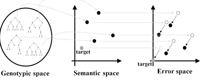
1 Individuals are represented by trees (or any other structure like linear genomes, graphs, etc.) in the genotypic space. Each one of them maps into its semantics, identified by a point in the semantic space. The semantic is then translated by subtracting the target, obtaining a point in the error space. The target, which usually does not corre-spond to the origin of the Cartesian system in the semantic space,
corresponds to the origin in the error space by construction. . . 2 2 Representation of simple bi-dimensional error space. Individuals A
and B are optimally aligned, i.e. their respective error vectors are directly proportional. (x, y, θ) is the angle between the error vector of
A (as well as B) and the one of C . . . 8 3 Results on the training set. Comparison between the
pro-posed methods (Align Angle GP, Align Angle GSGP), standard GP and GSGP. Plot (a): Bioavailability; plot (b): Concrete; plot (c):
En-ergy; plot (d): PPB; plot (e): Toxicity. . . 22 4 Results on the test set. Comparison between the stage one
meth-ods (Align Angle GP, Align Angle GSGP), standard GP and GSGP. Plot (a): Bioavailability; plot (b): Concrete; plot (c): Energy;
plot (d): PPB; plot (e): Toxicity.. . . 23 5 Results on the training set. Comparison between the proposed
methods (Align Error Fitness, Nested Align No Mult), standard GP and GSGP. Plot (a): Bioavailability; plot (b): Concrete; plot (c):
En-ergy; plot (d): PPB; plot (e): Toxicity. . . 25 6 Results on the test set. Comparison between the proposed
methods (Align Error Fitness, Nested Align No Mult), standard GP and GSGP. Plot (a): Bioavailability; plot (b): Concrete; plot (c):
En-ergy; plot (d): PPB; plot (e): Toxicity. . . 26 7 Results on the training set. Comparison between the prososed
methods (Nested Align, Align and Nested Align 50), standard GP and GSGP. Plot (a): Bioavailability; plot (b): Concrete; plot (c):
En-ergy; plot (d): PPB; plot (e): Toxicity. . . 27 8 Results on the training set. Comparison between the proposed
methods (Nested Align, Align and Nested Align 50), ESAGP-1
and ESAGP-2. Plot (a): Bioavailability; plot (b): Toxicity; . . . 28 9 Results on the test set. Comparison between the proposed
methods (Nested Align, Align and Nested Align 50), standard GP and GSGP. Plot (a): Bioavailability; plot (b): Concrete; plot (c):
En-ergy; plot (d): PPB; plot (e): Toxicity. . . 29 10 Results on the test set. Comparison between the prososed methods
(Nested Align, Align and Nested Align 50), ESAGP-1 and ESAGP-2.
11 Results at final generation (200) of all proposed models on the test set. The three models with the lowest error for each test problem are
highlighted in grey. . . 30 12 Results concerning the program size. Comparison between the
pro-posed methods (Nested Align, Align and Nested Align 50), stan-dard GP and GSGP. Plot (a): Bioavailability; plot (b): Concrete;
plot (c): Energy; plot (d): PPB; plot (e): Toxicity. . . 31 13 Results on the training set. Comparison between the proposed
methods (Nested Align, Align and Nested Align 50), standard GP and GSGP. Plot (a): Bioavailability; plot (b): Concrete; plot (c):
En-ergy; plot (d): PPB; plot (e): Toxicity. . . 34 14 Results on the test set. Comparison between the prososed
methods (Nested Align, Align and Nested Align 50), standard GP and GSGP. Plot (a): Bioavailability; plot (b): Concrete; plot (c):
List of Tables
1 GP parameters used in the present experiments. . . 19 2 Description of the test problems. For each data-set, the number of
features (independent variables) and the number of instances
(ob-servations) are reported. . . 20 3 Description of the concrete data-set . . . 20 4 Description of the Energy data-set . . . 20 5 p-values of the Wilcoxon rank-sum test on unseen data, under the
alternative hypothesis that the samples do not have equal medians.
LIST OF ABBREVIATIONS
ESAGP Error Space Alignment Genetic Programming GP Genetic Programming
GSGP Geometric Semantic Genetic Programming GSO Geometric Semantic Operator
1
INTRODUCTION
In the last few years, the use of semantic awareness for improving Genetic Program-ming (GP) (Koza, 1992; Poli et al., 2008) became popular. A survey discussing large part of the existing semantic approaches in GP can be found in Vanneschi et al. (2014). In that survey, the existing work was categorized into three broad classes: approaches based on semantic diversity, on semantic locality and on semantic geometry. Among several other references, se-mantic diversity and sese-mantic locality, and their relationship with the effectiveness of GP, were investigated in depth in Nguyen (2011). On the other hand, the idea of studying semantic ge-ometry revealed itself about a decade ago (see for instance Krawiec and Lichocki (2009a)), and became a GP hot topic in 2013, when a new version of GP, called Geometric Seman-tic GP (GSGP) was introduced (Moraglio et al., 2012). GSGP uses new operators, called ge-ometric semantic operators (GSOs), instead of traditional crossover and mutation, and it owes part of its successes to the fact that GSOs induce a unimodal fitness landscape (Vanneschi, 2017) for any supervised learning problem, which will be explained further in Section 3.1. As pointed out in Moraglio et al. (2012), GSOs create much larger offspring than their parents and the fast growth of the individuals in the population makes evolution unbearably slow after few generations, making the system unusable. In Vanneschi et al. (2013), a possible workaround to this problem was proposed, consisting of an implementation of Moraglio’s operators that makes them not only usable in practice, but also very efficient.
In the last few years, GSGP was studied and improved in many different ways. One notable ex-ample is various attempts at improving geometric semantic crossover. For instance, in Oliveira et al. (2016), methods for distributing individuals in the search space in order to make geomet-ric semantic crossover more effective were developed. Also, in Pawlak et al. (2015), several different types of geometric semantic crossovers were discussed and compared. Very recently, new forms of GSOs were introduced, such as perpendicular crossover and random segment mutation (Chen et al., 2017). Also, in Pawlak and Krawiec (2017) a suite of competent op-erators that combine effectiveness with geometry for population initialization, mate selection, mutation, and crossover were proposed.
Few years after the introduction of GSGP, a new way of exploiting semantic awareness was presented as a possible improvement to GSGP in Ruberto et al. (2014) and further developed in Castelli et al. (2014b); Gonc¸alves et al. (2016). The idea, which is also the focus of this paper, is based on the concept of error space, exemplified in Figure 3, and it can be sketched by the following points. The semantics of an individual is herein defined as the vector of its output values on the training cases (Moraglio et al., 2012). Semantics can be represented as a point in a space, which will be referred to as semantic space. Each point in semantic space can be translated to error space by subtracting the target from it. In this way, for each individual, a new point is obtained, called error vector, and the corresponding space is called error space. The target, by construction, corresponds to the origin of the Cartesian system in the error space. In supervised learning, the target vector is also a point in the semantic space, but usually (unless the rare case where the target value is equal to zero for each training case) it does not correspond to the origin of the Cartesian system.
Figure 1: Individuals are represented by trees (or any other structure like linear genomes, graphs, etc.) in the genotypic space. Each one of them maps into its semantics, identified by a point in the semantic space. The semantic is then translated by subtracting the target, obtaining a point in the error space. The target, which usually does not correspond to the origin of the Cartesian system in the semantic space, corresponds to the origin in the error space by construction.
In Ruberto et al. (2014), it was proven that, given sets of individuals with particular character-istics of alignment in the error space (called optimally aligned, and optimally coplanar, individ-uals), it is possible to analytically reconstruct a globally optimal solution (this is explained in detail in Section 3.1). Given this, it makes sense to develop a new GP system whose objective is to evolve for optimally aligned, or optimally coplanar, individuals (instead of looking directly for an optimal solution, as in traditional GP). The first attempt at developing a system aimed at searching for optimally aligned, or optimally coplanar, individuals was presented in Ruberto et al. (2014), where the Error Space Alignment Genetic Programming (ESAGP) method was proposed. While ESAGP reported interesting results, it has the important limitation of con-straining the possible alignment only in one particular direction in the error space, which is prefixed a priori. This was done by selecting one attractor individual and measuring fitness as the angle of the individual to this attractor in error space (i.e. the level of optimal alignment of the two individuals). A solution to this limitation is, rather than evolving single programs, a GP can evolve sets of programs, with each set being treated as an individual, and with the goal of evolving individuals whose sets of programs are optimally aligned, or optimally coplaner (depending on the number of programs in the set). The first preliminary attempt to evolve individuals made of two expressions was Castelli et al. (2014b), where the Pair Optimization Genetic Programming (POGP) system was introduced. However, in Castelli et al. (2014b) se-vere limitations of POGP, which make it unusable in practice, were also reported, these will be explicated in Section 3.2.
The objective of this paper is to present new GP systems aimed at evolving sets of two pro-grams with the objective of generating optimally aligned individuals, and which are able to over-come all the limitations of POGP. The new systems will be compared to standard GP, GSGP and ESAGP on a wide set of complex real-life symbolic regression problems.
The rest of the paper is structured as follows:
1. Section 2 provides an introduction to the concepts of Genetic Programming, including Geometric Semantic Genetic Programming.
2. Section 3 reviews previous and related work, with particular focus on ESAGP and POGP, describing the known issues of POGP.
3. Section 4 describes the development of the final proposed methods (Align, Nested Align and Nested Align β), by describing three method development phases, each of which included multiple proposed methods, and with each phase aiming to overcome limitations of the previous phase’s proposed methods.
4. Section 5 presents the current experimental study, in which the experimental settings and test problems are described and the obtained results of each of the three research phases are discussed.
2
INTRODUCTION TO GENETIC PROGRAMMING
2.1 TRADITIONAL GENETIC PROGRAMMING
Machine learning is the use of computational algorithms to discover patterns in, and pull mean-ing from, data. Rather than hard codmean-ing an algorithm with specific rules for pullmean-ing information from a specific data-set, machine learning algorithms develop a program for interpreting the data from the data itself. Generally the goal is for the algorithm to create a program, or expres-sion, which the features of the data instances can be plugged into. Generally, machine learning problems can be separated into two categories, supervised and unsupervised learning. This paper will deal with supervised learning problems. In supervised learning a training data-set exists wherein for each data instance, a target is known. The target is the value one wishes to predict for each instance. The target may be a category, or, as in the test problems addressed in this paper, the target may be a real number value representing a specific measurement (the actual energy load of a specific building, for example). In supervised machine learning, the algorithm creates a model for predicting target values, based on the patterns in the training data-set and their relationship to the known target values. This model can then be applied to other data, from the same data-set or representing the same thing, which the model has never seen, and can be used to predict the target value for each data instance.
A common problem that can occur in the training process is overfitting to the training data. This means that the model developed is too highly attuned to the patterns within the training set. That is, the model is taking into account patterns that are specific to the training set only and are not actually found in the data-set, or population, as a whole. It is clear that this has occurred when a proposed model performs very well at predicting the target value on the training set but very poorly on a previously unseen portion of the data-set (test set). A poorer performance on the test set than the training set is expected and common, since the model was trained specifically for the training set, however when performance on the tests set is much worse on the test set, overfitting has likely occurred. The definition of much worse is specific to factors such as the problem, the user and the performance of other available models.
Genetic programming is an evolutionary computation machine learning technique; it consists of the automated learning of computer programs by means of a process inspired by the theory of biological evolution of Darwin. In genetic programming, a group, or population, of programs is evolved over generations. In the context of GP, the word program can be interpreted in general terms,and thus GP can be applied to the particular cases of learning expressions, functions and, as in this work, data driven predictive models. In GP, programs are typically encoded by defining a set F of primitive functional operators and a set T of terminal symbols. Typical ex-amples of primitive functional operators may include arithmetic operations (+, −, ∗, etc.), other mathematical functions (such as sin, cos, log, exp), or, according to the context and type of problem, also boolean operations (such as AND, OR, NOT), or more complex constructs such as conditional operations (such as If-Then-Else), iterative operations (such as While-Do) and other domain-specific functions that may be defined. Each terminal is typically either a variable or a constant, appropriate to the problem domain. The objective of GP is to navigate the space of all possible programs that can be constructed by composing symbols in F and T , looking
for the most appropriate ones for solving the problem at hand. Generation by generation, GP stochastically transforms populations of programs into new, hopefully improved, populations of programs. The appropriateness of a solution in solving the problem (i.e. its quality) is ex-pressed by using an objective function (the fitness function). In synthesis, the GP paradigm evolves computer programs to solve problems by executing the following steps:
1. Generate an initial population of computer programs (or individuals).
2. Iteratively perform the following steps until the termination criterion has been satisfied: (a) Execute each program in the population and assign it a fitness value according to
how well it solves the problem.
(b) Create a new population by applying the following operations:
i. Probabilistically select a set of computer programs to be reproduced, on the basis of their fitness (selection).
ii. Copy some of the selected individuals, without modifying them, into the new population (reproduction).
iii. Create new computer programs by genetically recombining randomly chosen parts of two selected individuals (crossover).
iv. Create new computer programs by substituting randomly chosen parts of some selected individuals with new randomly generated ones (mutation).
3. The best computer program to appear in a generation is designated as the result of the GP process at that generation.
The standard genetic operators (Koza, 1992) act on the structure of the programs that represent the candidate solutions. In other terms, standard genetic operators act at a syntactic, or geno-typic level. More specifically, standard crossover is traditionally used to combine the genetic material of two parents by swapping a part of one parent with a part of the other. Consider-ing the standard tree-based representation of programs often used by GP (Koza, 1992), after selecting two individuals based on their fitness, standard crossover chooses a random subtree in each parent and swaps the chosen subtrees between the two parents, thus generating new programs, the offspring. On the other hand, standard mutation introduces random changes in the structures of the programs in the population. For instance, the traditional mutation operator, called sub-tree mutation, works by randomly selecting a point in a tree, removing whatever is currently at the selected point and whatever is below the selected point and inserting a new randomly generated tree at that point. As is clarified in Section 2.2, GSGPuses genetic oper-ators that are different from the standard ones, since they are able to act at the semantic level (Moraglio et al., 2012; Vanneschi, 2017) .
2.2 GEOMETRIC SEMANTIC GENETIC PROGRAMMING (GSGP)
The term Geometric Semantic Genetic Programming (GSGP) indicates a recently introduced variant of GP in which traditional crossover and mutation are replaced by so-called Geometric
Semantic Operators (GSOs), which exploit semantic awareness and induce precise geometric properties on the semantic space (Vanneschi, 2017). This methodology has been described by Castelli et al. Castelli et al. (2013) as follows. GSOs, introduced by Moraglio et al (Moraglio et al., 2012), are becoming more and more popular in the GP community (Vanneschi et al., 2014) because of their property of inducing a unimodal error surface (i.e. an error surface char-acterized by the absence of locally optimal solutions on training data) on any problem consisting of matching sets of input data into known targets (like for instance supervised learning problems such as symbolic regression and classification). To have an intuition of this property (whose proof can be found in Moraglio et al. (2012)), let us first consider a Genetic Algorithms (GAs) problem in which the unique global optimum is known and the fitness of each individual (to be minimized) corresponds to its distance to the global optimum (this reasoning holds for any em-ployed distance). In this problem, if for instance, box mutation is used (Krawiec and Lichocki, 2009b) (i.e. a variation operator that slightly perturbs some of the coordinates of a solution), then any possible individual different from the global optimum has at least one fitter neighbor (individual resulting from its mutation). So, there are no locally suboptimal solutions. In other words, the error surface is unimodal, and consequently the problem is characterized by a good evolvability. Now, let us consider the typical GP problem of finding a function that maps sets of input data into known target values (as was said, regression and classification are particular cases). The fitness of an individual for this problem is typically a distance between its predicted output values and the target ones (error measure). Geometric semantic operators simply de-fine transformations on the syntax of the individuals that correspond to geometric crossover and box mutation in the semantic space, thus allowing us to map the considered GP problem into the previously discussed GA problem.
Here, is reported the definition of the GSOs as given by Moraglio et al. (2012).
Geometric Semantic Crossover (GSXO) generates, as the unique offspring of parents T1, T2: Rn→ R, the expression:
TXO= (T1· TR) + ((1 − TR) · T2)
where TRis a random real function whose output values range in the interval [0, 1]. Analogously, Geometric Semantic Mutation (GSM) returns, as the result of the mutation of an individual T : Rn→ R, the expression:
TM = T + ms · (TR1− TR2)
where TR1 and TR2 are random real functions with codomain in [0, 1] and ms is a parame-ter called mutation step. Moraglio and co-authors show that GSXO corresponds to geometric crossover in the semantic space (i.e. the point representing the offspring lies on the segment joining the points representing the parents) and GSM corresponds to box mutation on the se-mantic space (i.e. the point representing the offspring lies within a box of radius ms, centered in the point representing the parent).
As Moraglio and co-authors point out, GSGP has an important drawback: GSOs create much larger offspring than their parents and the fast growth of the individuals in the population rapidly makes fitness evaluation unbearably slow, making the system unusable. In Castelli et al. (2015a), a possible workaround to this problem was proposed, consisting in an implementa-tion of Moraglio’s operators that makes them not only usable in practice, but also very efficient. With this implementation, the size of the evolved individuals is still very large, but they are repre-sented in a particularly clever way (using memory pointers and avoiding repetitions) that allows us to store them in memory efficiently. So, using this implementation, one are able to generate very accurate predictive models, but these models are so large that they cannot be read and interpreted. In other words, GSGP is a very effective and efficient “black-box” computational method. It is the implementation introduced in Castelli et al. (2015a) that was used with suc-cess in Castelli et al. (2015c,d) for the prediction of the energy consumption of buildings. One of the main motivations of this current work is the ambition of generating predictive models that could have the same performance as the ones obtained by GSGP or even better if possible, but that could also have a much smaller size. In other words, models that are both very accurate predictive models, as well as that are readable and interpretable.
3
PREVIOUS AND RELATED WORK
3.1 ERROR SPACE ALIGNMENT GP
In Ruberto et al. (2014), the concept of optimal alignment was introduced for the first time, together with a new GP method, called ESAGP (Error Space Alignment GP), that exploits it. Preparatory to the concept of optimal alignment is the definition of the error vector of a GP individual, i.e. the difference between the semantics of that individual and the target. The error vector is a point in a Cartesian space called error space, that is similar to the semantic space, but in which all points are translated in such a way that the target corresponds to the origin of the axis. According to Ruberto et al. (2014), two individuals A and B are optimally aligned if a scalar constant k exists such that eA = k · eB, where eA and eB are the error vectors of A and B respectively. From this definition, it is not difficult to see that two individuals are optimally aligned if the straight line joining their error vectors also intersects the origin in the error space, see Figure 2. As described in Ruberto et al. (2014), it is proven that given any pair of optimally
Figure 2: Representation of simple bi-dimensional error space. Individuals A and B are opti-mally aligned, i.e. their respective error vectors are directly proportional. (x, y, θ) is the angle between the error vector of A (as well as B) and the one of C
aligned individuals A and B, it is possible to reconstruct a globally optimal solution Popt. This is demonstrated as follows.
If two individuals are optimally aligned, then eA= k · eBthen SA− T = k · (SB− T ) where SA and SB are the semantic vectors of individuals A and B, respectively. Then, if T is the target vector:
SA− T = k · SB− k · T − T + k · T = k · SB− SA − T (1 − k) = k · SB− SA T = 1 (1 − k)· SA− k (1 − k)· SB
Thus with two optimally aligned individuals, it is possible to reconstruct a globally optimal solu-tion using Equasolu-tion (1):
Popt= 1
1 − k ∗ A − k
1 − k ∗ B (1)
Analogously, in Ruberto et al. (2014), it is also proven that given any triplet of optimally copla-nar individuals, it is possible to analytically construct a globally optimal solution; the models and results presented in this paper focus on evolving pairs of optimally aligned programs and recon-structing a solution using the equation above. The ESAGP method introduced in Ruberto et al. (2014) was composed by two GP systems: ESAGP-1, whose objective is looking for optimally aligned pairs of individuals, and ESAGP-2 whose objective is looking for triplets of optimally coplanar individuals. The biggest difference between these systems and traditional GP is that the search in ESAGP-1 and ESAGP-2 is not guided by the quality of the single solutions, but only on their alignment properties. Indeed, in principle, a globally optimal solution can by recon-structed analytically using pairs (respectively triplets) of solutions, as long as they are optimally aligned (respectvely coplanar) independently from their quality.
In practice, while running an algorithm which seeks to evolve optimally aligned individuals for the purpose of reconstructing a global optimal, it will be required to reconstruct the evolved solution from individuals that are not optimally aligned (i.e. an optimum has not been found). In this case the value of k must be approximated. In the models proposed in this paper k is calculated as follows: the ratio between EAand EB (EA/EB) at each coordinate is calculated. The median of these ratios is used as k, which is the method used in Ruberto et al. (2014). Several possible ways of searching for alignments can be imagined. In ESAGP, one direction, called attractor, is fixed and all the individuals in the population are pushed towards an align-ment with the attractor. The attractor used is a point in error space and the ’attraction’ is done by using the angle between the attractor and the error vector of the evolved expressions as the fitness measure, an optimum being any expression with an error vector with an angle of 0 to the attractor. The angle is minimized, so as to evolve individuals which are optimally aligned, or close to it, with the attractor. The idea is that this will evolve a population of individuals tending towards alignment with each other, and the attractor, in error space. The final product of the algorithm is an expression reconstructed, using Equation (1), from the two individuals most aligned with each other in the evolved population. In this way, ESAGP-1 and ESAGP-2 can maintain the traditional representation of solutions where each solution is represented by one program. The other face of the coin is that ESAGP-1 and ESAGP-2 strongly restrict what GP can do, forcing the alignment to necessarily happen in just one prefixed direction, i.e. the
one of the attractor. The issue here, is that the intuitive benefit of searching for aligned indi-viduals, rather than individuals as close as possible to the global optimum, is that theoretically, an optimal solution (optimally aligned individuals) can be located at any location in the search space. The single expression individuals method used in ESAGP, appears to restrict this bene-fit by the use of the attractor to define where the linearity must occur. Therefore, the concept of using individuals which are in fact vectors of expressions, was introduced as a method to more fully take advantage of the benefit of searching for optimally aligned individuals, this approach is the focus of the current research. An additional problem of ESAGP is the computational complexity and consequent slowness of the algorithm. This slowness is caused by the process employed by ESAGP-1 in order to find two error vectors that are aligned in the error space. The ESAGP-1 system represents individuals as simple expressions (like standard GP). It works by updating a repository of semantically different individuals evolved by GP at each generation and, for each semantically new individual created, checks whether it is optimally aligned with any of the individuals already in the repository. If a pair of optimally aligned individuals is iden-tified, the alogrithm terminates, otherwise, the algorithm continues. The models proposed in the current research avoid this heavy computational load because the set of expressions within one individual are only compared against each other, and the nature of the fitness function is intended to evolve these sets themselves to reach optimally alignment.
The ESAGP systems were also studied in Gonc¸alves et al. (2016), where the operators used to reach the alignment with the attractor were GSOs. The authors of Gonc¸alves et al. (2016) report severe overfitting for this new ESAGP version. For this reason the proposed methods in this paper focus on standard GP operators.
The objective of this paper is to relieve the constraint of ESAGP by defining a new GP sys-tem that is generally able to evolve vectors of programs. As already mentioned, a preliminary attempt is represented by POGP Castelli et al. (2014b), described below.
3.2 PAIR OPTIMIZATION GP
In Castelli et al. (2014b) Pair Optimization GP (POGP) was introduced. Limiting itself to the bi-dimensional case (i.e. to the case in which pairs of optimally aligned individuals are sought for), POGP extends ESAGP-1, releasing the limitation of forcing alignments in a prefixed direction discussed above. In POGP, individuals are pairs of programs, and fitness is the angle between the respective error vectors. This way, the algorithm can take advantage of the fact that optimal solutions can be found anywhere in the search space. Any multiple expression individuals that are generated have potential to evolve towards optimal alignment, regardless of their individual expressions distance from a global optimum, from each other, or from the expressions of the other evolved individuals.
From now on, for the sake of clarity, this type of individual (i.e. individuals characterized by more than one program) will be called multi-individuals.
In Castelli et al. (2014b), the following problems of POGP were reported: (i) generation of semantically identical, or very similar, expressions; (ii) k constant in Equation (1) equal, or
very close, to zero; (iii) generation of expressions with huge error values. These problems are discussed in further detail here:
Issue 1: generation of semantically identical, or very similar, expressions. A simple way for GP to find two expressions that are optimally aligned in the error space is to find two ex-pressions that have exactly the same semantics (and consequently the same error vector). However, this causes a problem once an attempt is made to reconstruct the optimal solution as in Equation (1). In fact, if the two expressions have the same error vector, the k value in Equa-tion (1) is equal to 1, which gives a denominator equal to zero. Also, it is worth pointing out that even preventing POGP from generating multi-individuals that have an identical semantics, POGP may still push the evolution towards the generation of multi-individuals whose expres-sions have semantics that are very similar between each other. This leads to a k constant in Equation (1) that, although not being exactly equal to 1, has a value that is very close to 1. As a consequence, the denominator in Equation (1), although not being exactly equal to zero, may be very close to zero and thus the value calculated by Equation (1) could be a huge number. This would force a GP system to deal with unbearably large numbers during all its execution, which may lead to several problems, including numeric overflow.
Issue 2: k constant in Equation (1) equal, or very close, to zero. Looking at Equation (1), one may notice that if k is equal to zero, then expression B is irrelevant and the reconstructed solution Popt is equal to expression A. A similar problem also manifests itself when k is not exactly equal to zero, but very close to zero. In this last case, both expressions A and B contribute to Popt, but the contribution of B may be so small to be considered as marginal, and Poptwould de facto be extremely similar to A. Experience tells us that, unless this issue is taken care of, the evolution would very often generate such situations. This basically turns a multi-individual alignment based system into traditional GP, in which only one of the expressions in the multi-individual matters. To truly study the effectiveness of multi-individual alignment based systems, these kind of situations must be impeded.
Issue 3: generation of expressions with huge error values. As previously mentioned, systems based on the concept of alignment in the error space could limit themselves to search-ing for expressions that are optimally aligned, without taksearch-ing into account their performance (i.e. how close their semantics are to the target). However, experience tells us that, if GP is given the only task of finding aligned expressions, GP frequently tends to generate expressions whose semantics contain unbearably large numbers. Once again, this may lead to several problems, including numeric overflow, and a successful system should definitely prevent this from happening.
3.2.1 Addressing Known Issues of POGP
The initial work of the current research explored the concept of using simple conditions to prevent these known issues of POGP: if these problematic numerical issues can be avoided, a multi-individual approach may be able to perform better than ESGAP, for the reasons discussed above.
An attempt was made to address POGP issues number 1, semantically identical individuals, and and 2, k very close to 0, by controlling for ’optimal’ values of k within the population. With an implementation of individuals as two expressions and a fitness being the angle between the two, the two expressions quickly converge to be almost the same (theta=0, k=1). Therefore, a minimum distance check was added. On initialization, when the second expression is added to an individual, first there was a check of distance between the two, if the distance was lower than a set minimum, a new expression was generated, until minimum distance is exceeded. This check also occurred on crossover (new parent selected until the minimum distance was met), and mutation (mutation recalculated, i.e. a new random tree generated). The results of these investigations was that theta still quickly reached values near 0, however the reconstructed solution was not an optimal one. It was determined that this was likely due to the evolution continuing to favour K = 1 individuals, it was doing this by selecting expressions with very large output values, therefore distances between two such expressions may be above the minimum distance set while K is still approximately 1. This problem persisted no matter the magnitude of minimum distance.
Next, a check for values of k greater 2 was implemented. However, this condition was found to be too strict and the algorithm was unable to create sufficient individuals which passed this restriction within a reasonable time.
Since ’forcing’ values of k of 2 or higher was not realistic, exploration of less restrictive values for k were tested. In all methods described below, a ’buffer’ around unacceptable values of k of +or − 0.02, is used. All individuals generated during initialization or evolution are rejected if k is within this buffer value range of 1, -1 or 0.
4
DESCRIPTION OF THE PROPOSED METHODS
4.1 OVERVIEW OF THE PROPOSED METHODS
The research was conducted in three phases, with each phase proposing variations on the proposed model of the previous phase, in order to overcome the model limitations observed in the previous phase. This section will describe the models proposed in each phase, and summarize the differences in performance on the test problems, in terms of test error, between the proposed models and standard GP and GSGP. Full results of all models are reported in Section 5.3. Finally, the top performing models identified after the three research phases will be described in further detail (see Figure 11 for a summary of model performance). In all cases, the methodology used for each model is the same, except for the differences that are explicitly noted.
4.1.1 Phase one
The first phase on research was based on the models discussed in Castelli et al. (2014b) and in Gonc¸alves et al. (2016). Two methods are introduced in this phase:
• Align Angle GP:Fitness is the minimization of the angle between the two expressions within the multi-individual. GP operators (mutation) are used.
• Align Angle GSGP: The only difference from Align Angle GP is that it uses semantic evo-lutionary operators (mutation), rather than traditional GP evoevo-lutionary operators. This was done to determine if one set of operators provided a clear and large benefit over the other in the context of using multi-individuals and error space alignment.
These methods are modeled after POGP, but with some differences in implementation designed to prevent the known problems of this model. As POGP had known research, Gonc¸alves et al. (2016) attempted to solve the known problems by limiting the primitive operators to + and −, however, results were not better than ESAGP. Since GP implementations using multi-individuals are subject to the known issues of POGP, and because initial testing of the current implementa-tion showed that the known problems did in fact exist when all standard mathematical operators were used (+, −, ∗, /), the use of a buffer around k of of + or − 0.02 was implemented for all models. All models were implemented with individuals with two expressions but theoretically all models could be extended to run with n expressions.
Mutation The mechanism implemented for applying mutation to a multi-individual is extremely simple: for each expression φi in a multi-individual, mutation is applied to φi with a given mu-tation probability pm, where pm is a parameter of the system. It is worth remarking that in this implementation all expressions φi of a multi-individual have the same probability of undergoing
mutation, but this probability is applied independently to each one of them. So, some expres-sions could be mutated, and some other could remain unchanged. The type of mutation that is applied to expressions is Koza’s standard subtree mutation Koza (1992).
Added to this “basic” mutation algorithm, is a mechanism of rejection, in order to help the selec-tion process in counteracting the issues discussed in Secselec-tion 3.2. Given a prefixed parameter that here is called call δk, if the multi-individual generated by mutation has a k constant included in the range [1 − δk, 1 + δk], or in the range [−δk, δk], then the k constant is considered, respec-tively, too close to 1 or too close to 0 and the multi-individual is rejected. In this case, a new individual is selected for mutation, using again the nested tournament discussed above. The combined effect of this rejection process and of the selection algorithm should strongly counteract the issues discussed in Section 3.2 and allow GP to evolve multi-individuals with k values that are “reasonably far” from 0 and 1.
Initialization. Nested Align initializes a population of multi-individuals using multiple execu-tions of the Ramped Half and Half algorithm Koza (1992). More specifically, let n be the number of expressions in a multi-individual (n = 2 in these experiments), and let m be the size of the population that has to be initialized. Nested Align runs n times the Ramped Half and Half algo-rithm, thus creating n “traditional” populations of trees P1, P2, ..., Pn, each of which containing m trees. Let P = {Π1, Π2, ..., Πm} be the population that Nested Align has to initialize (where, for each i = 1, 2, ..., m, Πi is an n-dimensional multi-individual). Then, for each i = 1, 2, ..., m and for each j = 1, 2, ..., n, the jthtree of multi-individual Πiis the jth tree in population Pi. To this “basic” initialization algorithm, is added an adjustment mechanism to make sure that the initial population does not contain multi-individuals with a k equal, or close, to 0 and 1. More in particular, given a prefixed number of expressions α, that is a new parameter of the system, if the created multi-individual has a k value included in the range [1 − δk, 1 + δk], or in the range [−δk, δk](where δkis the same parameter as the one used for implementing rejections of mutated individuals), then α randomly chosen expressions in the multi-individual are removed and replaced by as many new randomly generated expressions. Then the k value is calculated again, and the process is repeated until the multi-individual has a k value that stays outside the ranges [1 − δk, 1 + δk]and [−δk, δk]. Only when this happens, the multi-individual is accepted inside the population. Given that only multi-individuals of two expressions are considered in this paper, in the present experiments α = 1 is always used.
These proposed methods, which use angle as a fitness perform worse than GP or GSGP in four of the five test problems (the only exception was the PPB problem, where Align Angle GP performed better than GP and GSGP). The complete results of phase one are presented in Section 5.3.1.
4.1.2 Phase two
Given that the methods using angle as fitness were not improving on existing algorithms, the method of using reconstructed training error as fitness was explored. Additionally, a nested tournament selection was developed, in an attempt to further address the known issues with the alignment in error space method. These developments were represented in the two models tested in phase two:
• Align Error Fitness: Fitness is the minimization of the error on training data of the expres-sion ’reconstructed’ from the two expresexpres-sions of the multi individual.
• Nested Align No Mult: Fitness is a series of nested tournaments, as described below.
Full results for phase two are presented in Section 5.3.2. In terms of test error, Align Error Fitness and Nested Align No Mult performed better than GP and GSGP on the Energy Buildings and Concrete problems Nested Align No Mult showed the benefits of much faster improvement over GP and GSGP for the bio-availability problem, but still no improvement over ESAGP on the Bioavailability problem. Neither method showed an improvement on the toxicity or PPB problems compared to the results of StGP and GSGP.
4.1.3 Phase three
In an attempt to further improve the two methods developed in phased two, an additional mech-anism to prevent overly similar expressions was introduced: integer multiplication of one of the two expressions in each multi-individual. In addition, given that the methods proposed in phase one and phase two of the research consistently produce lower test error in initial generations than GSGP or StGP, even if the error after 200 generations is equal or higher, it seemed that it was possible that these methods were well suited to being initialization methods for GSGP or StGP. Therefore this was tested, in a preliminary fashion. As Nested Align showed good results on the widest range of models, this model was used as the initialization model.
• Align: Fitness is the minimization of the error on training data of the expression ’recon-structed’ from the two expressions of the multi individual. In addition, after selection and application of the genetic operator, one of the expressions is randomly selected to be multiplied by a random integer.
• Nested Align: Fitness is a series of nested tournaments, as described below. In addition, after selection and application of the genetic operator, one of the expressions is randomly selected to be multiplied by a random integer.
• Nested Align 50: Nested Align, described above, is used as an initialization method for GSGP. Nested Align is run for 50 generations, then, the expressions reconstructed from the evolved multi-individuals are used as the initial population for 150 generations of GSGP.
These three methods performed comparably to or better than to GP and GSGP for test error on all five of the test problems.
4.2 DETAILS OF THE FINAL PROPOSED METHODS
Given that the three models of phase three performed best on the largest number of test prob-lems, these models have been identified as the ’winning’ models. This section provides an in detail explanation of the methodologies of each of these winning models. In order to in-troduce the proposed methods in a compact way, Nested Align method is described first, and then the other methods are discussed by simply pointing out the differences between them and Nested Align.
4.3 NESTED ALIGN
Here, the selection of Nested Align is described, keeping in mind that no crossover has been defined for this method.
Selection. Besides trying to optimize the performance of the multi-individuals, selection is the phase that takes into account the issues of the previous alignment-based methods discussed in Section 3.2. Nested Align contains five selection criteria, that have been organized into a nested tournament. Let φ1, φ2, ..., φm be the expressions characterizing a multi-individual. Once again, it is worth pointing out that only the case m = 2 was taken into account in this pa-per. But the concept is general, and so it will be explained using m expressions. The selection criteria are:
• Criterion 1: diversity (calculated using the standard deviation) of the semantics of the expressions φ1, φ2, ..., φm (to be maximized).
• Criterion 2: the absolute value of the k constant that characterizes the reconstructed expression, as in Equation (1) (to be maximized).
• Criterion 3: the sum of the errors of the single expressions φ1, φ2, ..., φm(to be minimized). • Criterion 4: the angle between the error vectors of the expressions φ1, φ2, ..., φm (to be
minimized).
• Criterion 5: the error of the reconstructed expression Popt in Equation (1) (to be mini-mized).
The nested tournament works as follows: an individual is selected if it is the winner of a tourna-ment, that will be called T5, that is based on Criterion 5. All the participants in tournament T5, instead of being individuals chosen at random as in the traditional tournament selection algo-rithm, are winners of previous tournaments (that will be called tournaments of type T4), which
are based on Criterion 4. Analogously, for all i = 4, 3, 2, all participants in the tournaments of type Ti are winners of previous tournaments (that will be called tournaments of type Ti−1), based on Criterion i − 1. Finally, the participants in the tournaments of type T1 (the kind of tour-nament that is based on Criterion 1) are individuals selected at random from the population. In this way, an individual, in order to be selected, has to undergo five selection layers, each of which is based on one of the five different chosen criteria. Motivations for the chosen criteria follow:
• Criterion 1 was introduced to counteract Issue 1 in Section 3.2. Maximizing the semantic diversity of the expressions in a multi-individual should naturally prevent GP from creating multi-individuals with identical semantics or semantics that are very similar between each other.
• Criterion 2 was introduced to counteract Issue 2 in Section 3.2. Maximizing the absolute value of constant k should naturally allow GP to generate multi-individuals for which k’s value is neither equal nor close to zero.
• Criterion 3 was introduced to counteract Issue 3 in Section 3.2. If the expressions that characterize a multi-individual will have a “reasonable” error, then their semantics will be reasonably similar to the target, thus naturally avoiding the appearance of unbearably large numbers.
• Criterion 4 is a performance criterion: if the angle between the error vectors of the ex-pressions φ1, φ2, ..., φm is equal to zero, then Equation (1) allows us to reconstruct a perfect solution Popt. Also, the smaller this angle, the smaller should be the error of Popt. Nevertheless, experience tells us that multi-individuals may exist with similar values of this angle, but very different values of the error of the reconstructed solution Popt, due for example to individuals with a very large distance from the target. This fact made us conclude that Criterion 4 cannot be the only performance objective, and suggested to us to also introduce Criterion 5.
• Criterion 5 is a further performance criterion. Among multi-individuals with the same angle between the error vectors of the expressions φ1, φ2, ..., φm, the preferred ones will be the ones for which the reconstructed solution Popt has the smallest error.
4.4 DIFFERENCES BETWEEN ALIGN, NESTED ALIGN β AND NESTED ALIGN
Align. The difference between Align and Nested Align is that Align does not use the nested tournament discussed above. Selection in Align is implemented by a traditional tournament algorithm, using as fitness the error of the reconstructed expression Poptin Equation (1). Muta-tion and initializaMuta-tion in Align work exactly as in Nested Align. In this way, the only mechanism that Align has to counteract the issues described in Section 3.2 is to make sure that initializa-tion and mutainitializa-tion only create multi-individuals with a k value outside the ranges [1 − δk, 1 + δk] and [−δk, δk]. The motivation for the introduction of Align is that the nested tournament that characterizes Nested Align may be complex and time-consuming. Comparing the performance
of Nested Align to the ones of Align, one will be able to evaluate to importance of the nested tournament and its impact on the performance of the system.
Nested Align β. This method integrates a multi-individual approach with a traditional single-expression GP approach. More precisely, the method begins as Nested Align, but after β generations, the evolution is done by GSGP. In order to transform a population of multi-individuals into a population of traditional single-expression multi-individuals, each individual is re-placed by the reconstructed solution Poptin Equation (1). The rationale behind the introduction of Nested Align β is that alignment-based systems are known to have a very quick improve-ment in fitness in the first generations, which may sometimes cause overfitting of training data (the reader is referred to Ruberto et al. (2014); Castelli et al. (2014b); Gonc¸alves et al. (2016) for a discussion of the issue). Given that GSGP is instead known for being a slow optimization process, able to limit overfitting under certain circumstances (see Vanneschi et al. (2013)), the idea is transforming Nested Align into GSGP, possibly before overfitting arises. Even though a deep study of parameter β is strongly in demand, only β = 50 was tested in this paper. For this reason, from now on, the name Nested Align 50 will be used for this method.
5
EXPERIMENTAL STUDY
5.1 EXPERIMENTAL SETTINGS
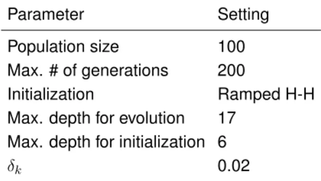
For each model, 30 runs were performed, each on a different randomly selected split of the data-set into training set (70%) and test set (30%). The parameters used are summarized in Table 1. Besides those parameters, the primitive operators were addition, subtraction, multipli-cation and division protected as in Koza (1992). The terminal symbols included one variable for each feature in the data-set, plus the following numerical constants: -1.0, -0.75, -0.5, -0.25, 0.25, 0.5, 0.75, 1.0. Parent selection was done using tournaments of size 5, with the exception of the models which use nested selection (i.e. Nested Align and, in the first 50 generations, Nested Align 50), which used a tournament of size 10 for each layer of the nested selection.
Parameter Setting
Population size 100
Max. # of generations 200
Initialization Ramped H-H
Max. depth for evolution 17 Max. depth for initialization 6
δk 0.02
Table 1: GP parameters used in the present experiments.
5.2 TEST PROBLEMS
The test problems that used in the present experimental study are five symbolic regression real-life applications. The first three (Bioavailability, PPB, Toxicity) are problems from drug discovery. Their objective is to predict a pharmacokinetic parameter (human oral bioavailability, plasma protein binding level and toxicity, respectively) as a function of a set of molecular descriptors of a potential new drug.
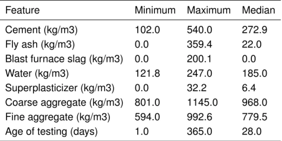
The fourth problem (called Concrete) has the objective of predicting the value of the concrete strength, as a function of some features of the material, particularly the supplementary materi-als in the makeup of the concrete mix (cement plus fly ash, blast furnace slag, and superplasti-cizer). The data-set is a representative selection of concrete with a variety of makeups of these ingredients. The variables of the data-set and their ranges are described in table 3.
Finally, the Energy problem has the objective of forecasting the value of the energy consump-tion, specifically, heating load (HL) in buildings simulated in Ecotect. HL is the amount of energy used for heating of the building. In particular, the data-set consists of eight independent vari-ables (or features) and 768 instances. Each instance is related to a particular feature building. The eight variables and the number of possible values for each are listed table 4 The
simu-data-set # Features # Instances Bio-availability Archetti et al. (2007) 241 206
PPB Archetti et al. (2007) 626 131
Toxicity Archetti et al. (2007) 626 234 Concrete Castelli et al. (2013) 8 1029 Energy Castelli et al. (2015b) 8 768
Table 2: Description of the test problems. For each data-set, the number of features (indepen-dent variables) and the number of instances (observations) are reported.
Feature Minimum Maximum Median
Cement (kg/m3) 102.0 540.0 272.9
Fly ash (kg/m3) 0.0 359.4 22.0
Blast furnace slag (kg/m3) 0.0 200.1 0.0
Water (kg/m3) 121.8 247.0 185.0
Superplasticizer (kg/m3) 0.0 32.2 6.4 Coarse aggregate (kg/m3) 801.0 1145.0 968.0 Fine aggregate (kg/m3) 594.0 992.6 779.5
Age of testing (days) 1.0 365.0 28.0
Table 3: Description of the concrete data-set
lated buildings were generated using Ecotect. All the buildings have the same volume, which is 771.75 m3, but different surface areas and dimensions. The materials used for each of the 18 elements are the same for all building forms. Other relevant features were also held constant with in the simulation, such as location, outside temperature, number of inhabitants. Original data-set has two target variables, cooling load and heating load. Original study (cite) shows that that the more successful at predicting the cooling load, so this was selected.
All these problems have already been used in previous GP studies Castelli et al. (2014b); Vanneschi et al. (2013); Castelli et al. (2014a, 2015b). Table 2 reports, for each data-set, the number of features (variables) and the number of instances (observations).
Features Description # of possible values
Relative compactness 12 Surface area 12 Wall area 7 Roof area 4 Overall height 2 Orientation 4 Glazing area 4
Glazing area distribution 6 Target variable (heating load (HL)) 586
5.3 EXPERIMENTAL RESULTS
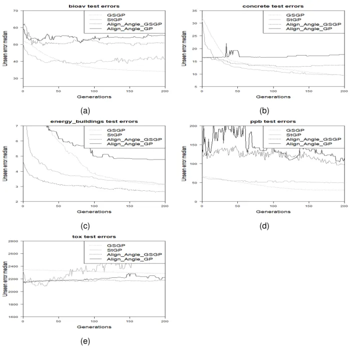
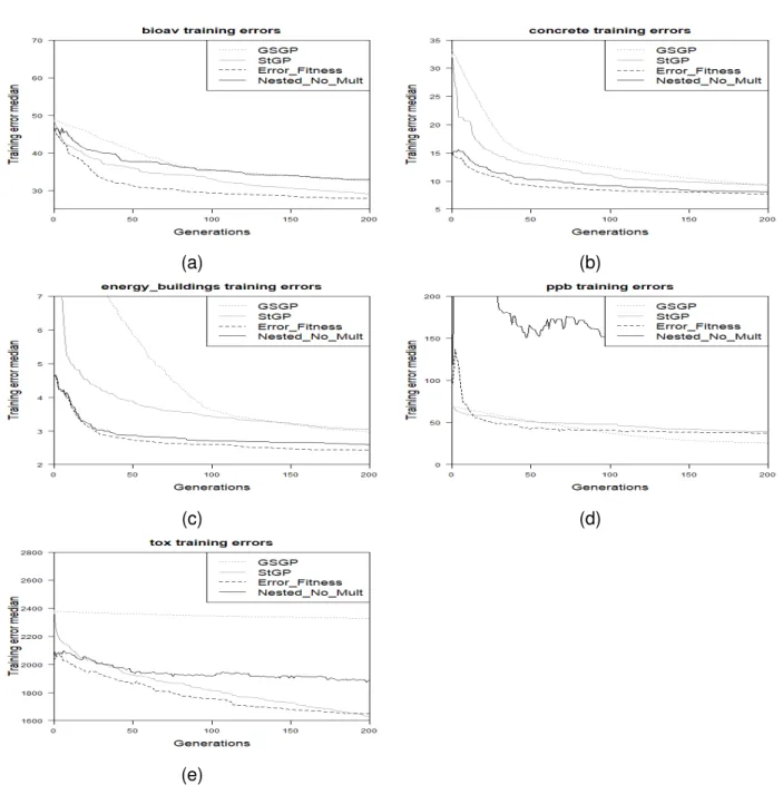
The results are separated by research phase. The training and test results for the proposed models for each stage are presented on separate graphs, along with the results obtained for GSGP and StGP on the relevant problem. In this way, the results for phase one, which compares Align GP and Angle GSGP to GSGP and StGP are reported in Figures 3 and 4. The results for phase two, which compares Align Error Fitness and Nested Align No Mult to GSGP and StGP are reported in Figures 5 and 6. The results for Align, Nested Align, and Nested Align 50 compared to GSGP and StGP, are reported in Figures 7 and 9, while the re-sults of Align, Nested Align, and Nested Align 50 compared to the rere-sults of ESAGP-1 and ESAGP-2 on the Bioavailability problem are presented in 8, and 10 (training and test errors, respectively).
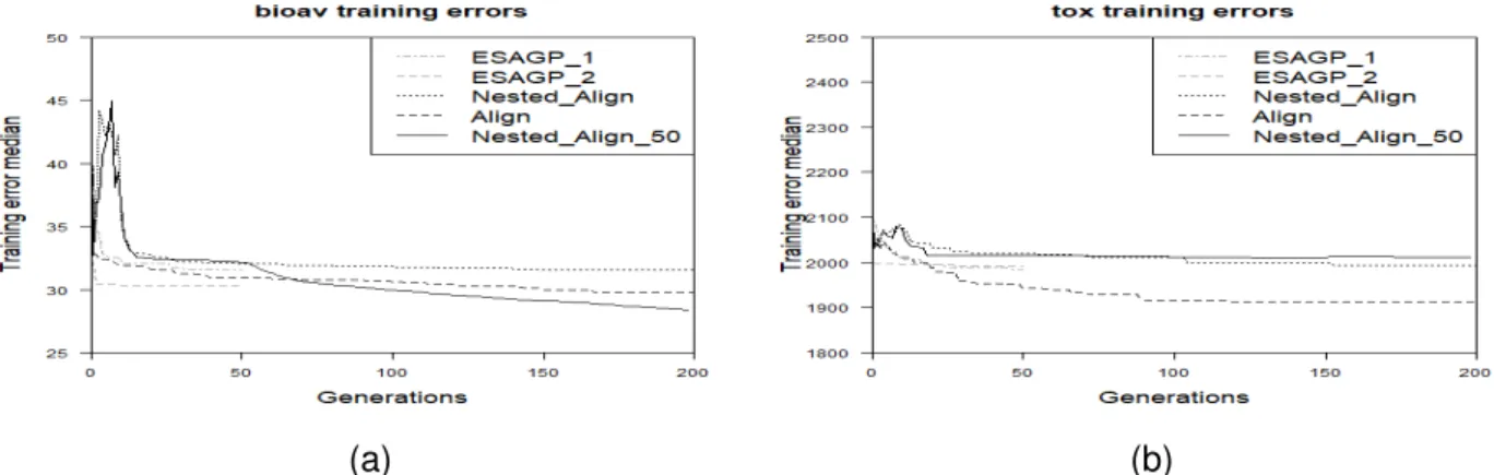
Concerning the ESAGP methods, the results have been taken directly from Ruberto et al. (2014), for comparison. In that paper, only results relative to training and unseen error on the Bioavailability and Toxicity data-sets were made available. For this reason, in Figures 8 and 10, plot (a) reports the results obtained on the Bioavailability problem and plot (b) reports the ones obtained on the Toxicity problem, and those figures do not contain any other plot in Figure 12, the results relative to the size of the programs (calculated as the number tree nodes).
In Figures 3 to 7, 9 and 10 (i.e. the ones where the proposed methods are compared to standard GP and GSGP), plot (a) reports the results obtained on the Bioavailability problem, plot (b) reports the ones obtained on the Concrete problem, plot (c) on the Energy problem, plot (d) on PPB, and plot (e) on the Toxicity problem.
Finally, Table 5 reports the results of the statistical tests performed on the obtained unseen errors.
(a) (b)
(c) (d)
(e)
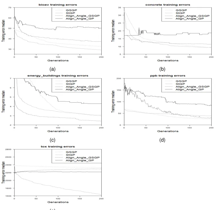
Figure 3: Results on the training set. Comparison between the proposed methods (Align Angle GP, Align Angle GSGP), standard GP and GSGP. Plot (a): Bioavailability; plot (b): Concrete; plot (c): Energy; plot (d): PPB; plot (e): Toxicity.
(a) (b)
(c) (d)
(e)
Figure 4: Results on the test set. Comparison between the stage one methods (Align Angle GP, Align Angle GSGP), standard GP and GSGP. Plot (a): Bioavailability; plot (b): Concrete; plot (c): Energy; plot (d): PPB; plot (e): Toxicity.
Training results of Align Angle GP and Align Angle GSGP compared to StGP and GSGP are presented in Figure 3. The only problem for which either of the phase one proposed mod-els gave the lowest training error, namely Align Angle GSGP performed best on the energy buildings data-set. For PPB, Align Angle GSGP training results are similar to, but not better than GSGP and StGP. For the Toxicity data-set, Align Angle GP and Align Angle GSGP per-form better than GSGP, however, StGP shows much better perper-formance than the other three models. For Bioavailability and Concrete, both GSGP and StGP perform better than the two proposed models.
Test results for Align Angle GP and Align Angle GSGP compared to StGP and GSGP are pre-sented in Figure 4. Again, there is only one problem for which either of the phase one proposed models gave the lowest test error, namely Align Angle GSGP performed best on the Energy data-set; Align Angle GP performs the worst on this problem, with GSGP and StGP providing errors between the errors of the two proposed models. On the Toxicity data-set, StGP reaches the lowest error of all of the models; the lowest error of StGP is reached before 50 generations, after which the model begins to over fifth and the error rises to be worse than all other models by generation 200. The two proposed phase one models begin at a lower error than StGP and GSGP, the errors remain steady for all 200 generations and never reaches error lower than the lowest StGP error. For Bioavailability, Concrete and PPB, both GSGP and StGP clearly perform better than the two proposed models.
5.3.2 Stage Two Experiment
The training errors of Align Error Fitness Nested Align No Mult compared to StGP and GSGP are presented in 5. The two proposed models of phase 2, Align Error Fitness Nested Align No Mult performed better than GSGP and StGP on the Energy and the Concrete problem, though on the Concrete problem all models performed quite similarly. Align Error Fitness had the lowest training errors on the Bioavailability problem, though the results are quite similar to StGP by the 200thgeneration. For Bioavailability and Concrete, both GSGP and StGP perform better than the two proposed models. On the PPB problem, GSGP provides the lowest training error and on the Toxicity problem, StGP provides the lowest training error by the 200th generation, however, the final training error of the Error Fitness model were almost identical and reached sooner than StGP.
The test errors of Align Error Fitness and Nested No Mult compared to StGP and GSGP are presented in 6. Both Align Error Fitness Nested Align No Mult performed best on the Concrete problem and the Energy problem; by the 200th GSGP and stGP reach similarly low (but not as low) errors on these problems, however, Align Error Fitness and Nested Align No Mult reach these levels much quicker. Error Fitness performs best on the Bioavailibility and Toxicity prob-lems. On the Bioavailability problem, GSGP reaches a similarly low to Error Fitness, but at a slower rate. Nested No Mult performs poorly on the other three test problems (Bioavailibility, PPB and Toxicity).
(a) (b)
(c) (d)
(e)
Figure 5: Results on the training set. Comparison between the proposed methods (Align Error Fitness, Nested Align No Mult), standard GP and GSGP. Plot (a): Bioavailability; plot (b): Concrete; plot (c): Energy; plot (d): PPB; plot (e): Toxicity.
(a) (b)
(c) (d)
(e)
Figure 6: Results on the test set. Comparison between the proposed methods (Align Error Fitness, Nested Align No Mult), standard GP and GSGP. Plot (a): Bioavailability; plot (b): Concrete; plot (c): Energy; plot (d): PPB; plot (e): Toxicity.
5.3.3 Stage Three Experiment
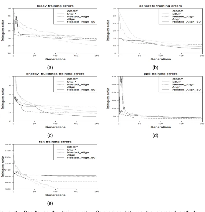
The results obtained are reported in Figures 7, 8, 9, 10 and 12.
(a) (b)
(c) (d)
(e)
Figure 7: Results on the training set. Comparison between the prososed methods (Nested Align, Align and Nested Align 50), standard GP and GSGP. Plot (a): Bioavailability; plot (b): Concrete; plot (c): Energy; plot (d): PPB; plot (e): Toxicity.
Figure 11 summarizes the the performance of all proposed models by reporting the test error at generation 200 for each model on each test problem. For each test problem, the three models with the lowest test error on that problem are highlighted in grey. The three proposed models of phase three performed in this top three on three out of five test problems. No other models performed in the top three on three or more test sets. In addition, all of the three models of phase three performed best on the Bioavailability and Tox test problems, which are the problems; these are the problems for which results for ESAGP-1 and ESAGP-2 are available
(a) (b)
Figure 8: Results on the training set. Comparison between the proposed methods (Nested Align, Align and Nested Align 50), ESAGP-1 and ESAGP-2. Plot (a): Bioavailability; plot (b): Toxicity;
as well.
Given that the three models of phase three, Align, Nested Align, and Nested Align 50, perform best on the largest number of test problems, these models have been identified as the ’win-ning’ models. These winning models were selected for were further analysis, specifically for comparison of tree sizes of the generated expressions as well as statistical significance testing between the results of these three models and GSGP and StGP.
Figure 7 shows, on the training set Nested Align 50 is the method that obtains the best re-sults on two problems over five (Concrete and Energy). On two of the other three problems (Bioavailability and Toxicity) the method that was able to find the best results was GSGP. Fi-nally, on the PPB data-set all the methods returned comparable results between each other, with a slight preference for Align. Remembering that, after 50 generations, Nested Align 50 “turns into” GSGP, an interpretation of these results is that, in general, GSGP is an appropriate method for optimizing training data, which is not surprising, given that GSOs induce a unimodal fitness landscape. In particular, the “switch” between the Nested Align algorithm and GSGP at generation 50 seems beneficial in much of the cases. This can be seen in the Bioavailability, Concrete and Energy problems, where a rapid improvement of the curve of Nested Align 50, looking like a sudden descending “step”, is clearly visible at generation 50. So, given that in the last part of the runs Nested Align 50 and GSGP are identical, Nested Align 50 prevails if the initial phase in which Nested Align was executed was beneficial. On the other hand, GSGP prevails if it was not. From the above discussed results, it can be concluded that it is benefi-cial on two problems, while it is not on two others (and it is irrelevant in the fifth of the studied problems, where Nested Align 50 and GSGP perform comparably). Concerning a comparison between the proposed methods and ESAGP-1 and ESAGP-2 (Figure 8), two considerations have to be made: first of all, in Ruberto et al. (2014) results were reported only until gen-eration 50, and those are the only ESAGP-1 and ESAGP-2 results available. Secondly, it is possible to ”speculate” that both ESAGP-1 and ESAGP-2 are outperformed by other methods both on the Bioavailability and on the Toxicity data-sets (more in particular, by Nested Align 50 and Align on Bioavailability and by Align on Toxicity). In fact, even though it cannot be known definitively, because data of the last 150 generations is not available, the curve of both the
(a) (b)
(c) (d)
(e)
Figure 9: Results on the test set. Comparison between the proposed methods (Nested Align, Align and Nested Align 50), standard GP and GSGP. Plot (a): Bioavailability; plot (b): Concrete; plot (c): Energy; plot (d): PPB; plot (e): Toxicity.
ESAGP methods, after a rapid decrease in the first 20 generations, seems to stabilize and to remain practically constant, approximately from generation 20 to generation 50.
Align, Nested Align, Nested Align 50: Now, let us discuss the results on the test set, start-ing from Figure 9. On the Bioavailability, PPB and Toxicity problems, the three proposed methods clearly outperform both GSGP and standard GP, with Nested Align 50 that is slightly preferable compared to the other two methods on Bioavailability and Align on Toxicity. On the Concrete and on the Energy problems, the method that performs better than all the others is Nested Align 50, and in both cases, also on the test set, a clear fitness improvement can be observed, looking like a sudden descending “step”, at generation 50, where the switch between Nested Align and GSGP takes place. In conclusion, on the test set all the three methods that
(a) (b)
Figure 10: Results on the test set. Comparison between the prososed methods (Nested Align, Align and Nested Align 50), ESAGP-1 and ESAGP-2. Plot (a): Bioavailability; plot (b): Toxicity;
Figure 11: Results at final generation (200) of all proposed models on the test set. The three models with the lowest error for each test problem are highlighted in grey.
have been introduced in this paper show reasonable results, improving the ones of GSGP and standard GP. Among those methods, Nested Align 50 seems the most preferable one, corrob-orating the intuition that Nested Align learns fast in the beginning, while the switch to GSGP allows us to continue the learning while limiting overfitting.
Concerning a comparison between the proposed methods and ESAGP-1 and ESAGP-2 (Fig-ure 10), what can be concluded using the data at available is that both ESAGP-1 and ESAGP-2 are outperformed by Nested Align 50 for the Bioavailability problem and by Nested Align 50 and Nested Align on the Toxicity problem. However, it is worth pointing out that, when dis-cussing the results on the test set, having data only until generation 50 strongly limits the possible conclusions. In fact, it is not known that, later in the run, the ESAGP methods will not begin to overfit, as it happens to, for instance, to Align on the Toxicity problem. Actually, on the Toxicity problem, Align outperforms both ESAGP-1 and ESAGP-2 in the first 50 generations, and only later in the run the test error of Align starts increasing. In synthesis, it is consid-ered that these conclusions (the ESAGP methods are outperformed by Nested Align 50 for the Bioavailability problem and by Nested Align 50 and Nested Align on the Toxicity problem) are the “best case” scenario for the ESAGP methods. If the until generation 200, were available, the picture for ESAGP could be even worse.
(a) (b)
(c) (d)
(e)
Figure 12: Results concerning the program size. Comparison between the proposed methods (Nested Align, Align and Nested Align 50), standard GP and GSGP. Plot (a): Bioavailability; plot (b): Concrete; plot (c): Energy; plot (d): PPB; plot (e): Toxicity.
generate much larger individuals compared to the other methods. This was expected, given that generating large individual is a known drawback of GSOs (Moraglio et al., 2012). The fact that in the first 50 generations Nested Align 50 does not use GSOs only partially limits the problem, simply delaying the code growth, that is, after generation 50, tree size is exactly as large as for GSGP. On the other hand, it is clearly visible that Align and Nested Align are able to generate individuals that are smaller than the ones of standard GP. Furthermore, after a first initial phase in which the size of the individuals grow, it can be seen that Align and Nested Align basically have no code growth (the curves of these two methods, after an initial phase of growth, are practically parallel to the horizontal axis). Last but not least, in all the studied problems the final model generated by Align and Nested Align has around only 50 tree nodes.