Cost-effective robot for steep slope
crops monitoring
Filipe Peixoto Mendes
Master in Electrical and Computers Engineering Supervisor: Prof. Pedro Luís Cerqueira Gomes da Costa Co-Supervisor: Prof. José Luis Sousa de Magalhães Lima Co-Supervisor: Dr. Eng. Filipe Baptista Neves dos Santos
A necessidade de eficiência no setor agrícola surge naturalmente de um progressivo aumento populacional e de crescente preocupação ambiental. Com este fim, existem esforços tanto da parte da investigação pública como da privada, focados no desenvolvimento de agricultura mais precisa e eficiente, onde recentes avanços tecnolóogicos permitem melhor gestão da atividade e uma utilização ótima de recursos. Apesar dos primeiros esforços no desenvolvimento de robôs para agricultura serem em tratores autónomos, com o preço reduzido dos veículos autónomos leves, especialmente drones, originou-se um aumento da atratividade deste tipo de veículos no novo paradigma de agricultura de precisão.
Os robôs terrestres agrícolas possuem a possiblidade de realizar uma multitude de tarefas no entanto, o seu desenvolvimento é particularmente desafiante devido a condições impostas pelo cenário agrícola, nomeadamente temperaturas elevadas, terrenos de forte inclinação, capacidade de comunicação limitada e estruturas não geométricas. Na região do Douro encontram-se vinhas instaladas ao longo das encostas, onde o grau de adoção de mecanização é baixo devido ao reduzido espaço para executar manobras e outras condições que tenham impacto na operação das máquinas.
O objetivo deste projecto é o desenvolvimento de uma plataforma robótica capaz de lidar com as dificuldades mencionadas. O robô utiliza um LIDAR 2D, um módulo GNSS, odometria e um IMU para realizar as tarefas de localização e mapeamento. Todos os sub-sistemas desenvolvidos, incluindo software, hardware e sistemas mecânicos são detalhados, juntamente com os procedimen-tos de teste e os resultados obtidos. De forma a reduzir o custo total, foi utilizada uma Raspberry Pi como computador principal. Também é conseguida a validação do algoritmo Cartographer SLAM em cenários diferentes e realizada uma análise de performance do algoritmo em componentes de baixo custo.
O resultado final é uma plataforma robótica open-source capaz de executar missões autono-mamente, onde é possível instalar componentes adicionais. Foi conseguido uma solução robusta de localização com componentes de baixo custo, uma solução de navegação e uma interface de utilizador com integração da aplicação QGroundControl.
An increasing population and the negative impact of agriculture on the environment drive the need for an agriculture more precise and efficient. Private and public research is emerging in the field of precision agriculture, where technological advancements enable better farm management and an optimal use of resources (e.g. Water, soil). Although first robotic developments focused on autonomous tractors, the cost reductions of light autonomous vehicles, especially drones, make these types of vehicles more attractive in the new paradigm of precision agriculture.
Whilst mobile agricultural ground robots bring many capabilities, their design is intrinsically challenging due to the harsh conditions imposed by the agricultural scenarios, such as high temperatures, terrain with slopes, difficult communications and non-geometrical location structure. In the Douro region, vineyards can be found installed in the steep-slope hills, where mechanization has a very low adoption rate due to lack of space for maneuvering and other conditions that impact machinery.
This work aims the development of a cost-effective open-source robotic platform, capable of handling the mentioned difficulties. The robot considers a 2D LIDAR, a Global Navigation Satellite System (GNSS) receiver module, odometry and an Inertial Measurement Unit (IMU) for self-localization and mapping. All the developed sub-systems, software, hardware and mechanical components are detailed, along with the testing procedures and obtained results. To reduce the overall cost, a Raspberry Pi computer is considered as the main processing unit. A validation of state-of-the-art algorithm Cartographer SLAM is done in different settings, along with an analysis of it’s performance on cost-effective hardware.
The final result was an open-source platform, capable of executing mission plans, which is to be fitted with additional hardware for the intended task. A robust localization solution with cost-effective hardware was achieved, along with a navigation stack and a user interface with integration of the application QGroundControl.
Gostaria de agradecer aos meus orientadores, Professor Pedro Costa, Professor José Lima e em especial ao Engenheiro Filipe Neves dos Santos, por me aceitarem no INESC TEC e orientarem a minha tese, foram imprescindíveis nesta jornada. Um agradecimento também à restante equipa do departamento de robótica, pelo feedback dado ao longo do semestre.
Aos meus amigos e amigas por todos os momentos de descontração, dificuldade, euforia e trabalho. Acompanharam-me neste último desafio de 5 anos, conhecem o meu melhor e o meu pior, e onde quer que a vida nos leve daqui para a frente, espero continuar a contar com o vosso apoio, da mesma forma que podem contar comigo.
Por fim, agradeço aos meus pais, Maria e Júlio, por todas oportunidades que, a muito sacrifício, me puderam providenciar. O mais profundo agradecimento por toda a compreensão, pelo conheci-mento, pela forma de encarar a vida que me transmitiram, a independência e a luta constante por um amanhã melhor, valores que moldam quem eu sou hoje e garantem o sucesso do meu futuro daqui para a frente.
Filipe Mendes.
Voltaire
1 Introduction 1
1.1 Motivation and Objectives . . . 2
1.2 Main contributions . . . 3
1.3 Thesis structure . . . 3
2 Background and Related Work 5 2.1 Sensors . . . 5
2.1.1 General Design Considerations . . . 6
2.1.2 Laser rangefinder . . . 7
2.1.3 Global Navigation Satellite System . . . 9
2.1.4 Dead Reckoning Sensors . . . 10
2.1.5 Cameras . . . 10
2.2 Localization and Motion Estimation . . . 11
2.2.1 Dead Reckoning . . . 12
2.2.2 Visual Odometry . . . 13
2.2.3 2D Laser Rangefinder Methods . . . 14
2.2.4 Beacon based localization . . . 14
2.3 Fusion and Estimation Algorithms . . . 15
2.3.1 State and Belief . . . 16
2.3.2 Markov and Kalman . . . 17
2.3.3 Kalman Filters . . . 17
2.3.4 Markov Filters . . . 18
2.3.5 Simultaneous Localization and Mapping . . . 19
2.4 Robot Motion . . . 19
2.4.1 Motion Planning . . . 19
2.4.2 Obstacle Avoidance . . . 20
2.5 Agricultural Robots . . . 20
2.5.1 Field Robot Event entries . . . 20
2.5.2 Conclusions . . . 21
2.5.3 Other solutions . . . 22
3 Approach and Developed Algorithms 23 3.1 Simultaneous Localization and Mapping . . . 23
3.1.1 SLAM methods analysis and comparison . . . 24
3.1.2 SLAM Configuration and Tuning . . . 28
3.1.3 Integration of GNSS data . . . 30
3.2 Motor Configuration and Control . . . 31
3.2.1 Controller Configuration . . . 32
3.2.2 Motor Driver ROS Node . . . 32
3.2.3 Odometry Model . . . 34
3.2.4 Odometry Calibration . . . 35
3.3 Sensor Acquisition . . . 35
3.4 Mission . . . 35
3.4.1 Mission Control Node . . . 36
3.4.2 Conversion between coordinates . . . 37
3.4.3 QGroundControl and the MAVLINK Protocol . . . 39
3.5 Navigation . . . 40
3.6 Final ROS Architecture . . . 41
3.7 Chapter Summary . . . 41
4 Hardware and Components 43 4.1 Processors . . . 44
4.2 Controllers . . . 44
4.3 Sensors . . . 44
4.3.1 2D LIDAR . . . 45
4.3.2 Inertial Measurement Unit . . . 45
4.3.3 GNSS Receiver . . . 46 4.4 Traction . . . 47 4.4.1 Motor Sizing . . . 48 4.4.2 Traction components . . . 50 4.5 Power . . . 51 4.6 Costs . . . 52 4.7 Final Assembly . . . 53 4.8 Chapter Summary . . . 53 5 Experimental methodology 57 5.1 Indoor Testing . . . 57 5.2 Outdoor Testing . . . 59 5.2.1 SLAM Testing . . . 60
5.2.2 IMU in the SLAM task . . . 61
5.2.3 Performance in the Raspberry Pi . . . 64
5.2.4 Comparison between Cartographer SLAM and Hector SLAM . . . 64
5.2.5 Mission Testing . . . 65
5.3 Final Testing . . . 67
5.3.1 Data collection and SLAM calibration . . . 67
5.3.2 Indoor Navigation . . . 70
5.3.3 UMBMARK Method . . . 70
5.4 Chapter Summary . . . 71
6 Conclusions and Future Work 73 6.1 Conclusions . . . 73
6.2 Limitations and Future Work . . . 74
2.1 Range estimation by measuring phase shift. Image from Siegwart’s book [7]. . . 8
2.2 One dimensional rangefinder measuring two objects and different distances and how it reflects and projects to the sensor. . . 8
2.3 Visual diagram of the pinhole camera model. The camera’s aperture is simplified to a point and no lens is assumed, so it becomes a first-order approximation for the two-dimensional mapping of a three-dimensional scene. Image from Wikipedia [10]. 11 2.4 Trilateration using 3 beacon (left) and Triangulation using 2 beacons (right) . . . 15
2.5 State representations of Kalman, Grid and Particle estimation, respectively. . . . 19
2.6 Floribot, The Great Cornholio and Beteigeuze respectively. . . 21
3.1 General Software Architecture. . . 24
3.2 Cartographer map with wheel odometry (Top) and Cartographer map without wheel odometry (Bottom) . . . 26
3.3 Hector SLAM map . . . 27
3.4 Trajectory estimation in Cartographer with wheel odometry (top left), without wheel odometry (top right) and Hector SLAM (bottom) . . . 27
3.5 On the top, the not tuned result. On the bottom is the tuned version. The blue line represents the estimated trajectory of the robot. . . 31
3.6 System overview of the Cartographer SLAM- . . . 32
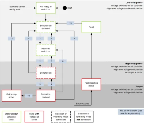
3.7 Motor power state machine according to the CAN in Automation standard. . . 33
3.8 Class Diagram of the twist_can_pkg node. . . 33
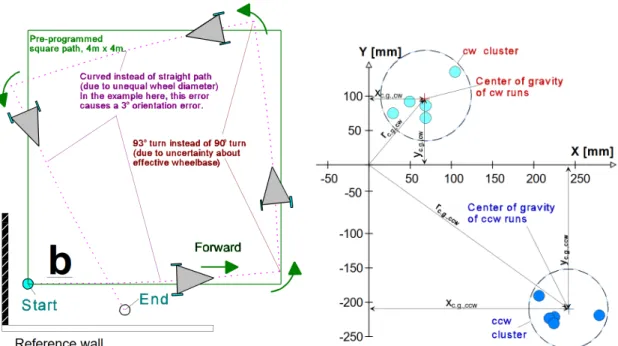
3.9 Illustration of the UMBMARK procedure and the resulting gravity centers of the errors. [14] . . . 36
3.10 Class diagram of the qgc_interface node. . . 37
3.11 State machine of the node that controls the mission. e represents the error to the next goal. . . 38
3.12 The longitude and latitude zones in the Universal Transverse Mercator system.. . 38
3.13 Upload and Download of the MAVLINK protocol [70]. . . 39
3.14 State machine of the navigation node. . . 40
3.15 Result of the ROS command rqt_graph which shows the nodes and topics they exchange. . . 42
4.1 Components and electrical interfaces. . . 43
4.2 Raspberry Pi 3 Model B. . . 44
4.3 Nanotec C5-E-2-09 Motor Controller. . . 45
4.4 Hokuyo URG-04LX-UG01 Scanning Laser Rangefinder. . . 46
4.5 Adafruit BNO055 Absolute Orientation Sensor . . . 46
4.6 IMU connected to the USB to serial adapter. . . 46
4.7 GNSS receiver with a soldered USB cable with an integrated converter chip. . . . 47
4.8 One wheel model with no friction force considered. Fg is the force exerted by gravity and Ft is the force that induces forward motion, . . . 48
4.9 Power scheme for a single wheel. . . 49
4.10 Nanotec DB59C024035-A BLDC Motor. . . 50
4.11 Neugart WPLE60-32 planetary gearbox. . . 51
4.12 Nanotec BWA-1.5-6.35. . . 52
4.13 On the top, the platform mid-way built. On the left, the built motor support. On the right, the motor electronics mounted under the platform. . . 54
4.14 Photograph of the final robot assembly. . . 54
4.15 3D CAD model of the platform. . . 55
5.1 Experimental setup mounted on a plywood, mounted on a pushcart . . . 58
5.2 Obtained maps from the first floor of the electrical engineering department, on the top is the output without IMU data and below with. . . 58
5.3 Capture of Linux htop command. Each number on the left represents a core in the processor, the percentage represents their current utilization. . . 59
5.4 Google maps capture of the parking lot and photograph of the area next to the INEGI building. . . 60
5.5 Map obtained from the parking lot. . . 60
5.6 Curve point where the scans are insufficient for proper SLAM. The matched points are represented by the white dots. . . 61
5.7 Car row passing and curve obtained from the parking lot, with an accurate SLAM output. . . 62
5.8 Map obtained from a path between natural vegetation and a dirt parking lot. . . . 62
5.9 Map obtained from row of cars in parking lot, without fusion of IMU data. Green boxes highlight "jumps" in the trajectory estimation. . . 63
5.10 Map obtained from a path between vegetation and a parking lot, without fusion of IMU data. . . 63
5.11 Map obtained from row of cars in parking lot, without fusion of IMU data. On the top is the Hector SLAM result and on the bottom Cartographer’s. Green boxes highlight "jumps" in the trajectory estimation. . . 65
5.12 Map obtained from a path between vegetation and a parking lot, without fusion of IMU data. On the top is the Hector SLAM result and on the bottom Cartographer’s. 65 5.13 Passed trajectory from ROS to QGC. . . 66
5.14 Goal points set in QGC. Distance errors (in meters) are, respectively: 19.26; 17.00; 18.09; and 14.3. Angle errors (in degrees) are: 46.75; 159.85; -120.03; and -48.10 66 5.15 Obtained maps, of the -1 floor of the Electrical Engineering department, after calibration of the algorithm in a simulated environment. . . 68
5.16 Map obtained from the robot in an online situation. . . 68
5.17 Outdoor map captured in the parking lot. . . 69
5.18 Capture of Linux htop command, with global part active along with the rest of the robot’s systems. . . 69
2.1 From Siegwart’s book [7, chap. Perception]. Classifies sensor by use, the
technol-ogy used, proprioceptive/exterocpetive (PC/EC) and active/passive (A/P) . . . 6
3.1 Average latency between laser scans and pose output running on a laptop. . . 28
3.2 Average latency between laser scans and pose output running on a Raspberry Pi 3B. 28 4.1 Specifications of the C5-E-2-09 Motor Controller. . . 44
4.2 Specifications of the Hokuyo URG-04LX-UG01 Scanning Laser Rangefinder. . . 45
4.3 Specifications of the GPS MOUSE - GP-808G. . . 47
4.4 Weight of the components and the vehicle’s total. . . 48
4.5 Specifications of the Nanotec DB59C024035-A motor. . . 50
4.6 Specifications of the Neugart WPLE60-32 planetary gearbox. . . 51
4.7 Specifications of the Nanotec BWA-1.5-6.35. . . 51
4.8 Power consumption of each component and estimated battery duration. . . 52
4.9 Price list of the components used in this project. . . 53
5.1 Weights used in the indoor testing. . . 59
5.2 Weights used in the outdoor testing. . . 64
5.3 Localization frequency, mapping frequency, average and maximum latency between scans and pose output. . . 64
5.4 Final (resumed) parameter list obtained from Cartographer’s calibration. . . 69
5.5 Parameters obtained from calibrating the navigation. . . 70
5.6 Values obtained from the UMBMARK method. . . 71
2D Two-dimensional 3D Three-dimensional
API Application Programming Interface BLDC Brushless DC
DGNSS Differential Global Navigation Satellite System EKF Extended Kalman Filter
FRE Field Robot Event
GNSS Global Navigation Satellite System GPS Global Positioning System
IMU Inertial Measurement Unit
INESC TEC Institute for Systems and Computer Engineering, Technology and Science IO Input/Output
IoT Internet of Things LED Light Emitting Diode
LIDAR Light Detection And Ranging RGB-D Red Green Blue - Depth ROS Robot Operating System RTK-GNSS Real-Time Kinetic GNSS
SLAM Simultaneous Localization and Mapping TOF Time-of-flight
UTM Universal Transverse Mercator
Introduction
An increase in population and growth rates, doubling since the 1960’s, combined with fast improve-ment of life expectancy in a world where approximately half of the global population’s calorie intake originates from agricultural products [1], strongly drives the need for an increased and more efficient agriculture activity. In an activity highly dependent on manual labor and amount of land, scalability becomes constrained, and trades between sustainable growth and environmental damage surge [2].
Technological advancements in robotic technologies, allied to a sensor price decrease, enable the development of cost effective robotic solutions, not only to overcome manual labor costs, but also to improve crop quality, resource efficiency, as well as environmental sustainability.
In the last years, multiple groups around the world have applied different automation solutions (e.g. sensor networks, manipulators, ground vehicles and aerial robots) to diverse agricultural tasks (e.g. planting and harvesting, environmental monitoring, supply of water and nutrients, and detection and treatment of plagues and diseases). [3, chap. Introduction]
Robots play an important role in the shift towards precision agriculture, especially in open-field farming (opposed to greenhouse farming). However, agricultural environments present a need for more robust and adaptable robots, capable of operating in varying conditions, harsh terrain with high unpredictability and other special requirements (e.g. careful harvesting of produce). Solutions often used in the industrial settings, where it’s possible even to design the plant to reduce the robot’s limitations, are often not appropriate for agriculture due to the reduced structured scenario and control. The lack of permanent natural features (wall, corners) challenges the localization algorithms, imposing the usage of complex localization algorithms to deal with dynamic changes. Some of the common challenges when designing open-field agricultural robots reside firstly in the careful design of locomotion systems and the corresponding mechanical project. Ground robots must be able to traverse terrain with a variety of perturbations and changes in ground texture (e.g. bumpy or soft terrain), unpredictable obstacles (e.g. branches or stones) and in some cases changes in terrain (e.g. from gravel to dirt).
Vision-based technologies are challenging in a setting naturally filled with noise, for example when detecting a fruit, it must be able to distinguish between it and leaves, branches, stems, stones and other naturally present elements in an environment with different lighting conditions and weather [4]. Recent improvements in vision-based control, algorithms and technology bring better performance in vision dependent applications, such as harvesting [5], or localization using natural feature detection in locations where the Global Navigation Satellite System (GNSS) signal isn’t always available or accurate [6].
1.1
Motivation and Objectives
One of the challenges in agricultural robotics is achieving a cost-effective ground robot, able to fulfill monitoring and other tasks autonomously, such as acquiring crop quality maps, apply pesticide, harvest or prune.
The steep-hill environment of river Douro’s mountain vineyards imposes bigger challenges than typical agricultural environments. Since Global Navigation Satellite System (GNSS) availability is low in steep-hills due to loss of line-of-sight in high elevation terrains (some moments with less than five satellites in view), the usual localization problem solution that involves Differential GNSS (DGNSS) is out of question. This brings the need of using other localization strategies and approaches.
To deal with these issues, in 2017, surges the project RoMoVi - Modular and Cooperative Robot for Vineyards. This project is being developed by Tekever (leader), INESC TEC and ADVID. The RoMoVi project aims to develop robotic components as well as a modular and extensible mobile platform, which will allow in the future to provide commercial solutions for hillside vineyards, capable of autonomously executing operations such as monitoring and logistics.
RoMoVi is aligned with the agricultural and forestry Robotics and IoT R&D line, called AgRob, being developed at INESC TEC (http://agrob.inesctec.pt). AgRob R&D focuses on developing robotic and IoT solutions for the agricultural and forestry sectors, considering the Portuguese reality. Based on both the RoMoVi and AgRob’s results and vision, a necessity for an open-source robot was identified, with the following features:
• Wheeled differential locomotion;
• Platform with basic sensors: LIDAR, IMU and GNSS receiver; • Assembling cost lower than 3000e;
• Capacity to carry a payload of 20kg; and,
• Small dimension so it can be used on Field Robot Event competition;
To accomplish this goal, it was required to develop robotic software sub-systems in the Robotic Operative System (ROS), select their interfaces and integrate with selected mechanical and electrical components. The project can be divided into three main tasks:
• Project and implementation of a robot platform for agriculture.
• Analysis and integration of existing ROS packages for localization and mapping. • Development of a user interface for mission planning and tracking the robot’s status.
1.2
Main contributions
The main contribution of this work is an open-source, low cost, simple and robust robot able to autonomously monitor crops using simple sensors, also usable on the Field Robot Event compe-tition. This work is publicly available athttps://gitlab.inesctec.pt/CRIIS/public/ agrobv19.
The second contribution of this work was the integration and validation of Cartographer -Simultaneous, Localization and mapping (SLAM) module - considering a cost-effective agricultural robot. Further, a comparison between Cartographer and Hector SLAM was performed.
The third contribution of this work is the development of a ROS package containing an API for sending commands via a CAN interface, for the Nanotec C5-E motor controller. This package is currently configured for translating ROS standard velocity commands and actuating on a two-wheel differential drive robot.
The fourth contribution is a ROS package which integrates the application QGroundControl, using the MAVLINK protocol over UDP, accepting mission plans and publishing the waypoints in the robot’s local coordinate frame.
The final contribution is the integration of GNSS data with Cartographer’s 2D SLAM problem. A pull request was submitted and is currently awaiting review.
1.3
Thesis structure
Besides the introduction, this thesis contains 5 more chapters. In chapter2, fundamentals of modern robotics are explored along with state-of-the-art technologies. In chapter3, the developed algorithms, solutions and software are presented. Chapter4details the hardware and components used, along with their interfaces and assembly. Chapter5describes the conducted experiments and their results. Finally, chapter6presents the conclusions, limitations, and suggestions for future work.
Background and Related Work
First and foremost, Autonomous Mobile Robots by Siegwart and Nourbakhsh [7] clearly provides the essentials of mobile robotics, and a launch point into more advanced topics. As such, it was used as a solid basis for comprehension of the topics described in the following chapter.
Autonomous navigation is one of the most challenging abilities required by mobile robots, since it depends on it’s four fundamental tasks: Perception, the robot must acquire and interpret the necessary data; Localization, the robot must determine it’s position; Cognition, the robot must take the decision on how to achieve it’s mission; and finally Motion Control, where the robot must correctly adjust it’s actuators in order execute the planned path.
This chapter was divided based on the aforementioned tasks and it’s content was tailored based on the systems that will be used in this project. First, an examination of the sensors is presented, followed by an analysis of localization techniques then, a view of the state-of-the-art estimation algorithms concluding then with motion planning strategies. Finally, existing solutions for the proposed problem are examined, both academic and commercial.
2.1
Sensors
Any autonomous mobile system must be able to acquire knowledge about itself and the surrounding environment. This challenge only worsens when considering outdoor operating environments due to various reasons, but mainly due to the necessary increase in range of the robot’s sensors and the introduced complications that naturally derive from an unstructured environment. In order to better understand how these technologies support mobile robotics, Everett’s book Sensors For Mobile Robots: Theory and Application[8] was essential as it presents an overview of both the theory of sensor operation as well as practical considerations when designing a system.
There are a variety of sensors for many different applications in robotics, as shown in table2.1. The sensors approached in this section were chosen for their relevance to the thesis, since these are the most popular sensors in low-cost agricultural ground mobile robotics, as will be later shown in this report, and also since these will be used in the development of the project. First, general considerations about the choice of sensors in mobile robots is presented, followed by an analysis
of operating principle, their main specifications, their limitations and their use in mobile robotics, both general and similar applications to this thesis.
Table 2.1: From Siegwart’s book [7, chap. Perception]. Classifies sensor by use, the technology used, proprioceptive/exterocpetive (PC/EC) and active/passive (A/P)
2.1.1 General Design Considerations
Each type of sensors possess their own unique specifications which should be balanced against the final system’s application, but there are still general traits that can be used to define and compare sensors. The following considerations were extracted from Everett’s [8] book:
• Field of View - Width and depth of sensing field.
• Range Capability - Minimum, maximum and maximum effective range. • Accuracy and resolution - Must fulfill the system’s requirements.
• Ability to detect all objects in environment - Some objects or surfaces may interfere with normal sensor operation. Environment conditions, noise and their interference should also be considered.
• Real-time operation - Update frequency, often related with the system’s speed. For example, an obstacle avoidance system much detect the object with a certain advance in order to execute security measures.
• Concise, easy to interpret data - The output of the data should be adapted to the application (too much data can also be meaningless). Problems here can be reduced by preprocessing the input data.
• Redundancy - Multi-sensor configurations should not be useless in case of loss of a sensing element. The extra sensors can also be used to improve the confidence level of the output. • Simplicity - Low-cost, modularity, easy maintenance and easy upgrades are all desirable
traits.
• Power Consumption - Must be in check with the intended system’s power limitations on a mobile vehicle (Both power and battery capacity wise).
• Size - It’s weight and size should be in check with the intended system.
However, theoretical characterization of the sensors is not enough since system’s frequently have restrictions in integration and field operation. Therefore expert information and field testing provided by the manufacturer should be consulted when designing such a mobile system.
2.1.2 Laser rangefinder
Laser rangefinders, also known as LIDARs, uses a laser beam to measure distances to objects using a time of flight (TOF) principle, either using a pulsed laser and measuring the elapsed time directly (not commonly used since it requires resolution in the picoseconds range) or by measuring the phase shift of the reflected light. Another manner is using a geometrical approach and a photo-sensitive device, or array of devices, in order to accomplish optical triangulation.
Phase-shift measurement One approach for measuring the TOF where the sensor transmits amplitude modulated light at a fixed frequency, is measuring the phase shift between the emitted beam and the received reflection. A diagram explaining phase shift measurements is presented in figure2.1, where distance to target is calculated as such:
D= λ
Figure 2.1: Range estimation by measuring phase shift. Image from Siegwart’s book [7].
Optical triangulation Uses a geometric approach by projecting a known light pattern (e.g single point, multi-point, stripe pattern, etc.) and capturing it’s reflection using a position-sensitive device. Then, with known geometric values, the system is able to use triangulation in order to measure the object’s distance to sensor (Fig.2.2). Optical triangulation is also used in 2D and 3D LIDARs, by projecting known light patterns and estimating the target’s shape and position by evaluating the distortion caused in the pattern.
Figure 2.2: One dimensional rangefinder measuring two objects and different distances and how it reflects and projects to the sensor.
Laser rangefinders are some of the most precise sensors used in robotics with precision in the millimeter range but, its precision comes at a high cost in comparison with other rangefinding technologies (e.g. ultrasound). Even though laser-based sensors have relatively high immunity
to noise, it’s use in outdoor, unstructured or somewhat structured environments is limited due to varying factors, from environmental conditions such as fog or systematic limitations when detecting, for example, an optically transparent object.
The main characteristics to be considered when considering laser rangefinders should be its minimum and maximum range, it’s scan angle, the angular (when applicable) and distance resolution.
2.1.3 Global Navigation Satellite System
GNSS or Global Navigation Satellite System is a satellite beacon navigation system that provides location and time information worldwide. One example is the NAVSTAR Global Positing System (GPS), owned by the United States government, launched in 1978 by the U.S. Department of Defense, and started exclusively for military applications. It was then progressively allowed for civilian use during the 1980s.
The GPS is usually composed by three segments:
• Space Segment: Composed by 24 to 32 satellites, in medium Earth orbit, with an orbital period of approximately 12 hours. Their orbits are arranged in a way that there is direct line-of-sight with at least 6 satellites at any time of the day.
• Control Segment: Provides support for GPS users and the space segments. Synchronizes space and user segment, so that transmissions are done with syncronized time stamps, guaranteeing that the system performs as intended.
• User Segment: GPS receiver with an antenna, processing and a precise clock.
This system uses trilateration with the time-of-flight of principle in order to determine it’s current position. In theory, in order to obtain the current location, 4 satellites are required (intersection of 4 spheres), although with 3 satellites (intersection of 3 spheres is two points) the location is deduced since one of the points will be far above or below the earth’s surface and can be excluded. In practice, a higher number of satellites within line-of-sight of the receiver will substantially increase it’s precision, although it’s still around a couple meters.
Since each satellite continuously sends it’s current location and time, a user only needs a passive GNSS receiver. The continuous transmission is low-power so one of it’s limitations is requiring direct line-of-sight to at least 4 satellites, making this system unusable in indoor systems without further adaptations. Theses factors make the use of GNSS popular for robots used in open-spaces and unmanned aerial vehicles.
GNSS cannot be used as a standalone localization technology, but developments around overcoming some of the precision limitations have used a fixed terrestrial station that is calibrated to know it’s position with high accuracy (e.g. 24 hour calibration by use of a constellation map) and providing the data to the mobile robot, which corrects it’s position [9]. This technique is known as Differential DGSS (DGSS).
2.1.4 Dead Reckoning Sensors
Dead Reckoning, in mobile robotics, is the process of estimating one’s current position by taking a previous known position and evaluating it’s evolution based on the robot’s dynamics (i.e. speed and acceleration). Dead reckoning in robotics is typically achieved using wheel odometry and an IMU (Inertial Measurement Unit). Most ground-based autonomous robots use Dead Reckoning as a baseline for navigation due to it’s high update frequency and then periodically correct it using other localization technologies (e.g. GNSS).
2.1.4.1 Optical Encoders
Optical incremental encoders are rotary encoders that use a light emitter (typically LED), a patterned mask, a disk and a sensor in order to determine the angular velocity and position of a motor, shaft or a wheel. Largely used in mobile robotics for motor control and Dead Reckoning. Since they are the most popular solution for measuring angular speed and shaft position and have avast range of applications, the development was pushed for high-quality and low-cost encoders, which greatly benefited mobile robotics.
The main specification when considering optical encoders is its resolution, which usually comes at a higher cost. Typical limitations are noise sensitivity at extremely low-speed, its finite resolution and errors introduced by discretziation as well as other approximations in odometry equations.
2.1.4.2 Inertial Measurement Unit
Inertial Measurement Units combine three sensors in order to acquire enough information to estimate the orientation, position, and velocity. Typical 9 degrees of freedom IMUs incorporate:
• Three-axis Magnetometer - Provides three dimensional orientation referenced to the earth’s magnetic field. Has limited performance in indoor and high EM noise environments. • Three-axis Gyroscope - Provides an angular speed referenced to the corresponding axis,
which can be then integrated to estimate the robot’s current pose and relative motion. • Three-axis Accelerometer - Measures it’s proper acceleration, with an output that gives the
direction and magnitude of the acceleration vector. Single and double integration provides us with complimentary speed and position information, respectively.
Although there are heavy limitations in the IMU’s performance, especially regarding sensitivity to noise and integration errors, their small size, low power consumption, and low cost make these sensors extremely popular in a number of robotics applications.
2.1.5 Cameras
Vision provides us, as well as robots, large amounts of information about our environment and allows for task realization in dynamic environments. It plays a role in many of a robot’s typical tasks
such as localization, mapping, object recognition, obstacle avoidance and navigation. Therefore significant efforts were made in the development of vision-based systems and it’s first stage, the camera.
Focusing on navigation, the pinhole model (fig:2.3) is essential in order to better understand how cameras can be used to obtain three-dimensional space information and how it’s projected into the image plane. Although the model doesn’t account for some of the sensor’s distortions (e.g. discretization and lens deformation), it is a sufficient approximation for a variety of applications in computer vision.
Figure 2.3: Visual diagram of the pinhole camera model. The camera’s aperture is simplified to a point and no lens is assumed, so it becomes a first-order approximation for the two-dimensional mapping of a three-dimensional scene. Image from Wikipedia [10].
There are three type of camera’s typically used in mobile robotics:
• Projective cameras - Most common cameras, approximated by the pinhole projective model, from which they get their name, with it’s focal point being the center of the lens.
• Omnidirectional camera - Has a field of view that either covers the entire sphere of view or a circle in it’s horizontal plane. Used for visual odometry and visual SLAM [11].
• Fisheye Camera - Composed of a projective camera and a fisheye lens, in order to increase the field of view or make it omnidirectional. The introduction of the lens requires appropriate models, such as the proposed by Courbon et al. [12], as the pinhole model cannot be used. Using cameras to extract three-dimensional space information (including depth) is also possible. Murray and Little propose a Stereo Vision based system [13] for autonomous grid occupancy mapping of an indoor environment, a setup where two cameras are used and the relative position of the detections is triangulated. Stereo and monocular setups will be discussed later in the Visual Odometry subsection.
2.2
Localization and Motion Estimation
Before exploring each technique, the general robot localization problem must be considered along with a solution strategy in context of the considered setting in this thesis. As a robot moves from
a well-defined starting point, the robot keeps track of it’s movement through odometry. But, due to accumulation of the odometry errors (e.g. wheel slippage, undefined point of contact with the ground), the robot’s uncertainty about it’s current position increases. So, the robot must periodically correct it’s position with other localization sensors (LIDAR, GNSS or visual sensors) and use them to estimate it’s location relative to to it’s environment. This two-step process allows the robot to determine it’s position relative to a map. Here, the distinction between proprioceptive and exteroceptive sensors is evident, as they play roles in the two distinct steps, prediction and update.
In this section, Dead Reckoning, the evolution of wheel odometry calibration and error esti-mation methods are studied, both On-line and Off-line. Following, comes an analysis of the more recent area Visual Odometry, a description of state-of-the-art of 2D laser rangefinder techniques (here the focus is on 2D, since it will be used in this project), and finally Beacon Based Localization. IMU and GNSS were not be addressed in this section since their operational principles are simple and well-defined.
2.2.1 Dead Reckoning
Odometry is the use of information from motion sensors for estimating a robot’s change in position over time. Dead Reckoning uses information from proprioceptive sensors, wheel encoders and IMU, while visual odometry uses visual techniques and the change in images in order to estimate motion.
One of the most popular techniques for estimating the internal state and dynamics of a mobile robot is the use of wheel sensors in order to measure rotation speed and integrate in order to obtain the robot’s current position. Two categories can be identified of error sources in odometry: Systematic errors, caused by the system’s internal problems, which usually presents as a bias. Non-systematic errors, on the other hand, are caused by external factors and are independent of the system’s characteristics, making it unbiased (random).
2.2.1.1 Wheel Odometry Calibration
Calibration is the process of comparing the outputs of a device under test to a reference value and correcting the parameters of the system in order to minimize errors (systematic or non-systematic). Wheel Odometry calibration can be divided into two groups.
Off-line methods These methods use a previously established test path that is followed by the robot without corrections and then, using the difference between the actual position and the estimated position, compensate it’s systematic errors. Off-line methods’ main advantage is that they can be done without requiring any additional sensors, although the final pose must be still measured manually which may introduce further errors. The most popular method is UMBmark presented by Borenstein [14], where a closed rectangular trajectory allowing for calibration of some systematic errors, but it was surpassed by more recent calibration procedures such as Antonelli’s [15] least-squares methods and the procedure PC-method developed by Doh et al. [16].
On-line methods Here, calibration is accomplished in real-time by using external sensors to periodically correct the odometry. The probabilistic approach also makes them more robust and less drift biased, but intimately ties their performance to sensor performance and the used models. One of the first proposed algorithms was by Roy and Thrun [17], an algorithm that automatically calibrates as it operates, with the concept of life-long calibration. Most recent trends rely on the assumption of the Gaussian distributions of error and the extremely popular Kalman filters. Martinelli et al. [18] developed an algorithm that uses laser and vision information to simultaneously calibrate the estimations and characterize the systematic error.
2.2.2 Visual Odometry
Visual Odometry in robotics is a process used to estimate a robot’s pose and movement gby comparing a sequence of camera images. Recent developments in processors and graphic processors along with general increases in computational power have increased the attractiveness of Computer Vision and, to the mobile robotics community specifically, the research into motion estimation. The term Visual Odometry was first introduced by Nister [19] which uses a stereo (multi-camera) setup and presents his algorithm based on the Harris detector. In monocular setups, Yamaguchi et al. implemented a monocular camera with feature detection in order to realize ego-motion estimation. Both these approaches are separated into two main categories, Stereo Vision which uses more than one camera in order to capture depth information and Monocular Setups which use only one camera. These methods can also then be divided into feature-based methods or dense methods.
Monocular Camera Setups In single camera visual odometry systems, three-dimensional infor-mation must be extracted from two-dimensional data, allowing us to retrieve relative inforinfor-mation but not in an absolute scale. Translating the data to a three-dimensional absolute scale is possible using extra input from other exteroceptive sensors (IMU, LIDAR, wheel odometry,...). Here, the computation of the new frames and the new camera pose estimation must be done for every new image. Forster et al. [20] provides a method for motion estimation with small number of features and extracted and without costly matching techniques. One of the most currently popular SLAM monocular algorithm based on visual odometry was proposed in 2015 by Mur-Artal [21].
Stereo Vision Uses multiple cameras and triangulation of the detected features for estimation of motion. Since the distance between the two cameras (stereo baseline) is fixed and known, the triangulation and estimation process is more accurate than it’s monocular counterparts. The most important developments for stereo vision were done in the Mars Rover context, where the final version was developed by Cheng et al. [22]. A second version of Mur-Artal’s work called ORB-SLAM2 provides an expansion of his own method to stereo and RGB-D cameras [21]. One of the main disadvantages of stereo setups is the need for very precise calibration and baseline definition, since variations in the baseline measure strongly effects motion estimation accuracy. Another important consideration is the relation between the baseline distance and the distance of
features in the target scene (application dependent), where if the stereo baseline is much shorter, these methods become inaccurate.
Feature-based methods In computer vision, a feature is a fragment of data which is relevant for solving a specific task. In the visual odometry pipeline, research has focused on Feature Extraction, with the groundbreaking AlexNet as developed by Krizhevsky [23] and furthered by Szegedy et al. [24], both based on convolutional neural networks. Novel Feature Matching methods that are robust or invariant to scale, rotations and lighting conditions were also developed, the most notable being SURF [25] and SIFT [26].
Dense methods Also known as Optical Flow methods, use information from the whole image or an image’s subregions in order to perceive motion from sequential variation in images. Theses methods are losing popularity against their feature-based counterpart since dense methods are only suitable when dealing with motion in a small scale environment.
2.2.3 2D Laser Rangefinder Methods
Since a robot cannot use data solely from odometry for precise navigation due to unbounded error, one of the possible solutions for correction is the use of a 2D laser rangefinder, which is also commonly used for localization [27],[28],[29], map building [30] and collision avoidance [31].
Thrun suggests a model and intrinsic parameter estimation algorithm for laser rangefinders that include four types of measurement errors: small measurement noise, errors due to unexpected objects, errors due to failures to detect objects, and random noise [32].
A popular application of laser rangefinders in localization is line extraction for map building. The classic method for line extraction is the Hough Transform [33], but better performing alter-natives came through such as the RANSAC [34], and the Split-and-Merge which came from the computer vision community [35]. Feature extraction for map building, motion estimation with im-age matching, and SLAM have been the focus of recent developments in 2D laser rangefinders [36].
2.2.4 Beacon based localization
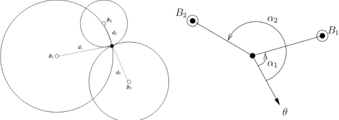
Another absolute localization strategy, useful in this case for the periodic correction of the odometry errors, is the use of beacons which act as absolute references in the map. Beacon based localization comes as an alternative to DGNSS (more expensive, GNSS signal dependent) or landmark based localization (detection of landmarks can be unreliable). This strategies’ biggest limitation is associated with indoor use, especially in narrow corridors and close-quarters complex maps. Also, a beacon alone is not enough to accurately ascertain the robot’s localization, where at least three are required. In order to deal with this situation beacon placement should also be carefully considered in order to maximize signal coverage on the operation area. Next, most common positioning methods are presented: Trilateration and Triangulation.
Trilateration Uses a method based on the distance to the beacons which is measured using the TOF principle. Theoretically, only 3 beacons are necessary to deduce the robot’s position, since the intersection of the three circles drawn from the distance will intersect in one point (fig.2.4). In practical applications the measurements are subject to noise and the returned location will be a region instead of a single point, so generally speaking an increase in the number of beacons will increase the accuracy of the localization prediction.
Triangulation This method uses the Angle of Arrival (AoA) principle to ascertain the robot’s position. Since it relies on the geometric properties of triangles, it theoretically only needs 2 beacons to function but in practice (Fig.2.4) more beacons are desirable. Although this technique requires less beacons and doesn’t require time synchronization between the beacons, the hardware necessary to precisely determine the angle of arrival of a transmitted wave is very expensive, which make these techniques undesirable for the robotics community.
Figure 2.4: Trilateration using 3 beacon (left) and Triangulation using 2 beacons (right)
Since both these techniques are subject to measurement errors, and typically return a point region instead of a definitive solution, another estimation algorithm must be used such as the EKF localization estimator which will described in the following section.
2.3
Fusion and Estimation Algorithms
When facing uncertainty in the study of the algorithms presented below, the book Probabilistic Robots [32], considered the standard reference for robotic navigation and mapping, provides a clear-cut analysis to the standard approaches used in robotics for estimation and fusion, SLAM, navigation and decision making.
First the fundamental concepts of modern localization methods are presented, followed by an analysis of the two popular categories of probabilistic localization methods, Kalman and Markov. Finally, the SLAM problem is defined along some of the most popular solutions.
2.3.1 State and Belief
As robots move away from the tightly controlled industrial setting into more dynamic and unstruc-tured environments, coping with uncertainty becomes a more important requirement in robotic systems. A probabilistic robot uses probability theory concepts to explicitly model the system and it’s uncertainty, posteriorly using the space of probabilistic possibilities to control the robot, instead of using one unique set of information that is assumed to be true. Since sensor outputs are only measurements of states and can be affected by errors, probabilistic methods prove themselves to be more robust and accurate.
The probability theory formulated by Bayes describes the robot’s Beliefs referenced to it’s States, Recursive Bayesian Estimation then estimates a system’s state based on it’s past state and beliefs.
2.3.1.1 State
State is a set of variables that describes a robot as well as the environment’s aspects that impact a known system. These variables may be static or dynamic and are used to describe both external or internal information. Examples of state variables used in robotics are:
• A robot’s pose given by six state variables, three Cartesian coordinates that indicate the robot’s position (length, width, height) and three Euler angles to describe the pose (roll, pitch and yaw). Also known as Kinematic state.
• The configuration of a robotic manipulator joints (linear, orthogonal, rotational,...) and their position at any point and time.
• Information regarding velocity and forces applied to a robot and it’s joints. Also known as Dynamic State.
• Location and features of objects, beacons, and landmarks in an environment. • Other information, such as the battery level of a battery-powered system.
2.3.1.2 Belief
As discussed before, a sensor doesn’t measure a state directly. Therefore, a probabilistic robot does not adjust it’s outputs directly based on the sensor data, but through the state information "guessed" from the sensor data. Thrun [32] defines beliefs as "A belief reflects the robot’s internal knowledge about the state environment.", and these beliefs are defined using probability theory as conditional probabilities. In this example state variables are represented as xt, all past measurements as z1:t and
all past controls as u1:t.
2.3.1.3 Bayes Filter
In order to better understand how more complex filters and algorithms work and how they bridge over to robotics, the analysis of the Bayes Filter Algorithm or Recursive Bayesian Estimator is essential since it provides the basis of the most popular estimation techniques such as the Kalman and Particle filter.
Algorithm 1 Bayes Filter
1: procedure BAYESFILTER(bel(xt−1), ut, zt)
2: for all xt do
3: bel(x¯ t) = ∑ p(xt|ut, xt−1)bel(xt−1)
4: bel(xt) = η p(zt|xt) ¯bel(xt)
return bel(xt)
In line 3, a belief of the current state is given based on the state’s transition model, it’s belief in the past state and the control inputs. It’s belief assigned to the state xt is based only on the past
belief of the state and the probability that the control ut induces a change from xt−1 to xt. This
step is usually called prediction as it only uses the state’s transition model and it’s inputs, with no regards to external measurements.
In line 4, the belief of the robot is updated taking into consideration the belief of the robot’s current state and the probability that the measurements zt were observed, which is then multiplied
by a normalization constant η. This adds an a correction to the predicted belief and is typically callled measurement update.
2.3.2 Markov and Kalman
Before diving deeper into each class, a brief introduction and comparison of both methods is necessary. First, Kalman filter localization models the system’s belief using a matrix containing Gaussian probability density functions, which can be defined by only its mean µ and it’s standard deviation σ . To update the Kalman Filter is to update the parameters of it’s Gaussian distribution. These algorithms are suited for continuous world representations, but are not stable in face of large displacements in position (e.g. collision, kidnapping). Second, Markov localization represents multiple points or regions and assigns probabilities for each of the robot’s possible poses. In the update step, the algorithm must update every considered point or region making Markov localization methods usually more computationally demanding.
2.3.3 Kalman Filters
The Kalman’s Filter [37] basic assumption is that the considered systems are linear, stochastic and ergodic, this means that although it’s output will be affected by random white noise, it’s statistical properties will be retained. Kalman Filter uses linear equations to deal with Gaussian distributions defined simply by their mean and variance. Kalman Filter’s proves effective in systems that can accurately be modeled by linear models and whose sensor error can be approximated to a Gaussian
distribution. But this restricts the algorithm to simple robotics problem in a controlled environment, so in order to empower the Kalman Filter, the Extented Kalman Filter was developed.
2.3.3.1 Extended Kalman Filter
In the Extended Kalman Filter, state transition and measurement models are first-order, differen-tiable functions. Instead of evaluating only linear equations, EKF evaluates the Jacobian (matrix of partial derivatives) of the models, where the state prediction and updates propagate through a non-linear system, while the errors propagate through a linearized Taylor’s series.
The EKF generally retains the benefits of the Kalman Filter regarding simplicity and compu-tational efficiency, but are still dependent on the accuracy of the approximation, since the filter’s performance and stability depend on keeping the uncertainty small.
It is also the most popular algorithm for state estimation and data fusion in robotics [38],[39], although EKF still faces performance issues when dealing with highly non-linear systems.
2.3.4 Markov Filters
Markov Filters Remove the assumptions used in Gaussian filters and use a finite set of points distributed throughout a specific region of space, each with an assigned probabilistic value. This makes Markov Filters more suitable when dealing with global uncertainty, feature matching and complex non-linear systems, trading off with computational demand tied to the number of parameters used in the model. Markov Filters can generally be divided into two classes.
Histogram Filters Which divide state-space regions and assign each one with a probability. A well-known implementation of this filter is the Grid Localization, where the regions are divided into squares each with an assigned probability. This filter has a particular trade-off: cell-size (and number) vs. computational cost. More modern solutions have proposed algorithms with variable grid sizes and shapes according to the robot’s current state [40].
Particle Filters Uses a distribution of samples, points called particles, spread around the robot’s localization (the denser, the more probable that the state falls into that region), each representing a possibility with assigned probability of the robot’s pose. The most popular particle filter technique, Monte Carlo Localization, was developed by Thrun et al. [41] in 2001, solving the global local-ization and the kidnapping problem in a robust and efficient way, while needing no feedback of it’s initial position if a map is provided. Although particle filters are generally a better solution than Kalman Filters, the required computational cost makes it unfit for low-cost systems.
Figure2.5shows a visual state representation of these the Kalman filter, the grid Markov filter and the particle filter.
Figure 2.5: State representations of Kalman, Grid and Particle estimation, respectively.
2.3.5 Simultaneous Localization and Mapping
The aforementioned algorithms are closely tied with mapping procedure, and are appropriate for problems either where a robot’s pose is known and the environment has to be mapped, or where the map of the environment is provided and the pose must be determined.
If a robot neither has been provided a map, neither it’s own pose, we arrive at a problem known as Simultaneous Localization and Mapping, which has been widely researched by the robotics community. One of the earliest and popular algorithms is based on the Extended Kalman Filter and is known as EKF-SLAM, but due to it’s high complexity and need for non-ambigous landmarks, it has been replaced as the de facto standard by FastSlam [42]. Great methods have also risen from the robotics vision community for solving the SLAM problem using visual odometry and mapping, such as the ORB-SLAM [21], PTAM [43] and RGBD-SLAM [44].
2.4
Robot Motion
Robot Motion is where the processed measurement data and the mission details are interpreted and used to make a decision, along with the following execution. Typical robot motion architectures are separated into three parts which will be addressed in this section: Motion Planning The robot’s path is planned; Obstacle Detection The robot must override the plan and take security measures in case of an obstacle; Task Execution The robot executed the planned path. In this work defined as Motor Control, since they are this system’s outputs.
2.4.1 Motion Planning
In the autonomous navigation process, path planning is one of the simpler challenges and was already heavily studied due to it’s applications in industrial robotics, where high speeds and big payloads require a precise control of the forces exerted on the manipulator’s joints. Since mobile robotics generally deals with low speeds, dynamics are not considered during path planning. Path planning should be adapted to the robot’s specific application which is also strictly tied with the
mapping process. A variety of strategies over the years emerged for solving this problem, and the most popular ones are described here.
Road map Theses techniques decompose the map into a graph network where the robot’s possible motions are simplified to a one-dimensional connection, simplifying the decision making to a shortest path graph problem. The complexity of Road map techniques lie on the obtained map decomposition, here the most popular techniques are the Visibility Graph [45], which returns the shortest possible path, and Voronoi diagrams [46] which calculates a path that maximizes the distance between the robot and obstacles.
Fuzzy navigation Approaches using Fuzzy logic are by far the most popular techniques used today, since their simplicity and versatility in defining heuristics and incorporating subjectivity allows the modification of conventional algorithms making them more robust [47], [48].
Cell decomposition Decomposes the space intro geometric areas and classifies them as either free or occupied by objects, then using a graph computes the trajectory by searching the graph. Recent successful methods use cells that change in shape and size over time, reflected on the uncertainty of the estimations [49]
2.4.2 Obstacle Avoidance
Obstacle avoidance focuses on a more local view of the trajectory, where paths are planned locally and giving particular importance to close rangefinding technologies. The most common approaches to obstacle avoidance are Bug algorithms [50], grid map occupancy avoidance [51] and potential fields [52].
2.5
Agricultural Robots
The analysis of existing solutions focused on the 15th and 16th editions of the Field Robot Event, an annual competition launched in 2003 by the University of Wageningen that puts robots to the test in a series of challenges (e.g. in-row navigation, mapping, weeding) that must be completed autonomously, with the caveat that GNSS is forbidden. Around 15 teams compete in the FRE every year and their solutions along with technical specifications of the robots are provided in the event’s proceedings [53]. From these proceedings standout examples were chosen and described below and then general conclusions about the competing robots are presented. Finally, three standout commercially available solutions are explored.
2.5.1 Field Robot Event entries
Floribotuses two front differential drive wheels with two swivel wheels behind, allowing for turns on it’s own axis. Highly scored (third place) using only a 2D laser rangefinder for navigation and
a camera for object recognition. It’s cost-effectiveness is surprising and is also merited to the implemented navigation algorithm based on potential field, where the plants create a repulsive field and the robot follows a preset list of a instructions introduced via mobile app.
The Great Cornholiouses a robot-platform "Volksbot" by the Fraunhofer Institute which is powered by two 150W DC motors using a skid-steer system which, while providing higher payload capacity, is still an inefficient method of locomotion. This solution uses encoders, an IMU and a 2D laser scanner for navigation as well as a camera for object recognition. Their navigation strategy uses a varying size grid occupancy method where the grid is considered occupied if the laser "hits" a plant more times than the threshold value.
Finally, Beteigeuze stands out as a heavy-weight (literally, the robot weights 40 kg) in the competition. It brings two 2D laser rangefinders, encoders, an IMU, 2 stereo cameras (camera + structured light) and a fisheye camera. Earning first place in the 2017 edition, it uses a single central motor to power it’s 4-Wheeldrive system. It also uses a central camera for the image processing and spatial information extraction for the "weeding" tasks.
Figure2.6shows the pictures of these three entries.
Figure 2.6: Floribot, The Great Cornholio and Beteigeuze respectively.
2.5.2 Conclusions
Here, the general conclusions of the agricultural robot’s market survey are presented:
Software Tools ROS is the most popular framework for developing the robot’s software. Another commonly used tool is MATLAB/Simulink and the robotics toolbox for developing algorithms then testing them inside MATLAB. Since MATLAB is based on C++, there is code portability directly to ROS which completes the development environment. Standout mentions in simulation software go to Gazebo and V-REP.
Localization Since in the competition the use of GNSS is banned, most entries use a 2D laser rangefinder for row detection fused with the odometry and IMU data for position estimation. But this is the setup which is used for the competition, since most agricultural robots cannot confidently rely on odometry and lasers only for navigation, most robots are also fitted with a DGNSS module that allows for precise localization within an open crop field.
Navigation Most of the implemented navigation algorithms were custom-made for this com-petition and examples are found based on potential fields, cell decomposition and mathematical methods such as using a least square estimator for regression fitting the line between the rows. Here, relevant solutions to the competition are found but real-world robust and reliable navigation is often more complex.
Motors and Traction The two most popular traction methods found were Ackermann Steering with it’s simple control, higher weight capacity and high efficiency (no wheel slip when turning); and the simple Differential Drive with passive casters, providing fast closed turns but also a lower weight capacity and more susceptibility to rough terrain (rough terrain makes the passive casters constantly bounce). Typical total motor power for both these systems are 200W to 300W.
Computers and Processors Most robot’s use a low-cost PC for high level control and algorithm processing (e.g. Raspberry Pi) combined with a micro-controller for low-level actuation and PID motor control. When the system requires visual algorithms, not only for object recognition but also odometry and extraction of 3D information, an Intel NUC, a desktop PC or other equivalent component is also installed.
2.5.3 Other solutions
Bosch offers a robot development platform that includes a robot designed for hard terrain, modular, with 4 independent wheel drive along with other software tools for simulation, logging,... This model uses a Differential GNSS technique with a base station and a receptor module called RTK-GNSS which is then fused with IMU data, enabling precision around 2cm. Bonirob is popular in both private and academic projects [54], [55].
Other important mentions which are focused on the vineyard context is the VinBot [56], combining a 3D LIDAR and an RTK-GNSS fused with IMU and wheel odometry data and VineRobot [57]. Both these robots allow for the user to monitor in real-time the vineyard’s quality parameters, improving both quality and optimizing management, and are closest to the proposed solution in this thesis.
Approach and Developed Algorithms
The main challenges of this thesis rely on the restrictions imposed by the project which can be divided into two: environmental and cost restrictions. The steep-hill environment of river Douro’s mountain vineyards pose three big challenges: Accuracy reduction from dead reckoning systems that naturally derive from the intended environment’s harsh terrain; Reduced GNSS availability and accuracy due to the steepness of the Douro’s wine-making regions; Difficult localization and navigation for safe route planning, avoiding damage to both the robot and the surrounding crops. Focusing on a low-cost system also brings many restrictions, but it’s main drawback is the reduction of computational power which strongly limits the choice of both localization and navigation algorithms.The proposed solution is here divided into two categories: Hardware, where the details of the components are exposed along with their electrical interfaces; And Software, where the focus is on the composition of the individual nodes and their responsibilities, then defining their inter-communication. This chapter will focus on the software development as well as the reasoning behind the chosen methods. Below (Fig.3.1, is the general software architecture composed by blocks that correspond to each of the robot’s main functions.
The localization and mapping system will use IMU, Odometry, GNSS and the LIDAR for solving the SLAM problem. The SLAM module will process the sensor data and feed it to the mission planning module. The mission planning module evaluates the tasks given and the current state of the robot in order to determine the robot’s next action, which is then fed to the navigation module along with position information from the SLAM module. The navigation module will then output to the motor driver in order to act on the robot.
3.1
Simultaneous Localization and Mapping
SLAM is the most challenging task in the mobile robotics field and each solution should be adapted to the intended environment. According to the specifications of the project, the SLAM algorithm should be reliable and robust as the solution for the absolute localization, able to process real-time measurements, while not being too computationally expensive as a solution, for the considered
Figure 3.1: General Software Architecture.
hardware. This section will present a comparison between two state-of-the-art algorithms, it’s choice, integration in the system, calibration, and developed modules along with obtained maps containing trajectory estimation.
3.1.1 SLAM methods analysis and comparison
SLAM methods for this project must fulfill two main criteria: Low computational cost and robustness when mapping and localizing in an unstructured environment. Two popular SLAM algorithms were identified that meet (or can be adapted) to fit this criteria. First, the massively popular Hector SLAM [58] developed in Dramstadt University in 2011 for the RoboCup Rescue competition, with the goal of providing sufficiently accurate mapping and self-localization while minimizing computational costs. It combines a 2D LIDAR and and IMU for full 2D motion estimation. Alternatively is Google’s Cartographer [59] introduced in 2016. Cartographer’s strong suits are the facilitation of integration of different sensors using only raw data (e.g. GNSS, IMU, 2D/3D LIDAR, Kinect, etc.) and its robustness for large-scale maps using loop-closure between pose and map. Cartographer’s SLAM can actually be divided into two, first the local SLAM, which frequently publishes sub-maps of the surrounding area, and global SLAM, whose job is to tie all its sub-maps consistently by periodically providing map constraints from the LIDAR scan matching and the odometry.
The logs used were provided by INESC TEC and extracted from the AGROBv16 in April 20 2018, in the vineyards of the University of Trás-os-Montes and Alto Douro, for comparisons in the intended environment. This data set is available athttp://vcriis01.inesctec.pt, named Data acquired by Agrob V16 @UTAD (20/04/2018), containing all the registered topics in the robot
at that time: Controller commands, video, pose and localization information, maps, and the data output of the sensors. The information used in these experiments was the IMU raw data, the laser scanner raw data and the filtered odometry.
3.1.1.1 Map comparison
All the maps extracted use the same thresholds for free and occupied cells in the published occupancy grid in order for a reasonable comparison to be established. In this case free cells (in white) have an occupancy probability lesser than 35% while occupied cells’ probability is larger than 65%.
Here three procedures are compared:
• Cartographer using a 2D LIDAR, IMU and wheel odometry; • Cartographer using a 2D LIDAR and IMU; and,
• Hector SLAM using a 2D LIDAR and provided odometry from wheel odometry and IMU. As can be seen in figures3.2and3.3, both of Cartographer’s maps are generally more immune to noise and low-height obstacles, attributing a lower probability to objects that are not repeatedly and consistently matched which as a consequence produces maps with finer detail of the environment’s strongest features (in this case the vineyards’ trunks). Considering scan matching depends on the pose estimation of the robot, the map produced by Cartographer when running with all sensors is more consistent with the environment due to the stability of the pose estimation when using wheel odometry. Second, although not observable in this map since it was only a short forward and back path in a larger vineyard, Cartographer’s periodic map loop closing allows for large and non-collinear robot paths while keeping the robustness of both the map and its pose estimation.
Hector map is more consistent when mapping features at a longer distance as can be seen in the map’s extremes, but since this project will be using a rangefinder with only a 5.6m range, it doesn’t present as an advantage.
3.1.1.2 Trajectory and pose estimation comparison
Since there is no ground truth provided, only a qualitative analysis is possible. Pose error compar-isons can be found in [60]. Both Cartographer and Hector provided a similar and consistent global pose estimation. In figure3.4, Cartographer’s pose estimation without wheel odometry becomes highly susceptible to IMU noise and vibrations originating from the rough terrain.
3.1.1.3 Computational cost
In tables3.1and3.2, the average latency between the laser scans and the output of the estimated pose is presented for the three methods considered, firstly in a modest machine, the laptop MSI CX-62 6QD with an Intel i5-6300, and secondly in the Raspberry Pi 3B which will be used for the


![Figure 3.13: Upload and Download of the MAVLINK protocol [70].](https://thumb-eu.123doks.com/thumbv2/123dok_br/15488767.1040865/57.892.243.698.703.1071/figure-upload-download-mavlink-protocol.webp)
