Francisco Miguel da Silva Vieira do Coito
Licenciado em Ciências da Engenharia Eletrotécnica e de Computadores
Study on the Development of an
Autonomous Mobile Robot
Dissertação para obtenção do Grau de Mestre em Engenharia Eletrotécnica e de Computadores
Orientador: Stanimir Stoyanov Valtchev, Prof. Doutor,
FCT-UNL
Co-orientador: Robert Babuska, Prof. Doutor, TU-Delft
Júri:
Presidente: Prof. Doutora Maria Helena Silva Fino Arguente(s): Prof. Doutor Luís Filipe Figueira de Brito Palma
Vogal(ais): Prof. Doutor Stanimir Stoyanov Valtchev
I
Copyright © 2014
Francisco Miguel da Silva Vieira do Coito,
A Faculdade de Ciências e Tecnologia e a Universidade Nova de Lisboa têm o direito, perpétuo e sem limites geográficos, de arquivar e publicar esta dissertação através de exemplares impressos reproduzidos em papel ou de forma digital, ou por qualquer outro meio conhecido ou que venha a ser inventado, e de a divulgar através de repositórios científicos e de admitir a sua cópia e distribuição com objetivos educacionais ou de investigação, não comerciais, desde que seja dado crédito ao autor e editor.
III
Acknowledgement
It is doubtful that anyone may arrive at the end of his dissertation without a good deal of help
along the way, I’m certainly no exception. High on the list of those to thank is my advisor,
Professor Stanimir Valtchev, for his patience and precious advice. Next on the list is my co-advisor Professor Robert Babuska, for welcoming me at Technishe Universiteit Delft (TU-Delft), to continue the development of my work, and Professor Gabriel Lopes, for his helpful counseling during my stay at TU-Delft.
It was a great pleasure to work with them. Their aid helped me to think carefully about my
work’s development. I also thank them for believing in me, for the scientific and technical
support, and for the motivation.
I would also like to thank all the members of the Departamento de Engenharia Electrotécnica (DEE) of Faculdade de Ciências e Tecnologia da Universidade Nova de Lisboa (FCT-UNL) and of the Department of Systems and Control (Delft Center SC) of Technishe Universiteit (TU) Delft.
All my thanks also to my teachers, colleagues, family and friends, who aren’t mentioned individually by name, for helping me to be who I am.
Abstract
V
Abstract
This dissertation addresses the subject of Autonomous Mobile Robotics (AMR). It is aimed to evaluate the problems associated with the orientation of the independent vehicles and their technical solutions. There are numerous topics related to the AMR subject. Due to the vast number of topics important for the development of an AMR, it was necessary to dedicate different degrees of attention to each of the topics.
The sensors applied in this research were several, e.g. Ultrasonic Sensor, Inertial Sensor, etc. All of them have been studied within the same environment.
Employing the information provided by the sensors, a map is constructed, and based on this map a trajectory is planned.
The Robot moves, considering the planned trajectory, commanded by a controller based on Linear Quadratic Regulator (LQR) and a specially made model of the robot, through a Kalman Filter (KF).
Resumo
VII
Resumo
O tema desta dissertação é Robótica Móvel Autónoma (AMR). Este trabalho tem como objetivo estudar problemas associados com a orientação dos veículos independentes e as suas soluções técnicas. Existem tópicos numerosos relacionados com o tema AMR. Devido ao vasto número de tópicos importantes para o desenvolvimento de um AMR, foi necessário dedicar diferentes graus de atenção a cada um dos tópicos.
Os sensores aplicados nesta pesquisa eram vários, por exemplo, Sensor Ultrassónico, Sensor Inercial, etc. Todos eles foram estudados no mesmo meio ambiente.
Usando a informação provenientes pelos sensores, um mapa é construído, e uma trajectória é planeada com base neste mapa.
Considerando a trajectória planeada, o Robot move-se seguindo os comandos por um controlador baseado no Regulador Linear Quadrático (LQR) e com um modelo do robot, baseado em Filtro de Kalman (KF).
Subject Index
IX
Subject Index
1 Introduction ... 1
1.1 Motivation ... 1
1.2 Problem Formulation... 2
1.3 Contributions ... 5
1.4 Dissertation Overview ... 5
2 Environment Perception – Ultrasonic Sensor ... 7
2.1 The Ultrasonic Sensor for distance measurements ... 7
2.2 Ultrasonic Sensor Features ... 9
2.2.1 Width of the Ultrasonic Sensor’s Acoustic Cone ... 9
2.2.2 Ultrasonic Sensor’s Measurement Readings ... 11
2.3 Target Detection ... 13
2.3.1 Use a Rotating Ultrasonic Sensor ... 13
2.3.2 Other ways to detect a Flat Surfaced Target ... 19
2.4 Summary ... 19
3 Mapping and Trajectory Planning ... 21
3.1 Environment Mapping... 21
3.1.1 Mapping and Localization of the Robot ... 22
Subject Index
X
3.1.3 EKF-SLAM Algorithm ... 25
3.1.4 An alternative Algorithm ... 27
3.2 Trajectory Planning ... 27
3.2.1 Reinforcement Learning ... 28
3.2.2 Implementation of the Trajectory Planner ... 34
3.2.3 Trajectory Smoother ... 35
3.3 Summary ... 38
4 Multi-rate Sensor Fusion Localization ... 41
4.1 Localization through Sensors ... 41
4.2 Multi-rate Sensor Fusion ... 42
4.2.1 Organizing the data ... 43
4.2.2 State Estimation ... 44
4.3 Off-Line Analysis ... 46
4.3.1 MR’s Dynamics ... 48
4.3.2 MR1’s main trajectory ... 49
4.3.3 MR2’s performed trajectories ... 56
4.4 Summary ... 60
5 Variance adaptive LQR Controller... 63
5.1 System Dynamics ... 63
Subject Index
XI
5.3 Adaptive Controller scheme ... 65
5.4 Kalman Filter ... 66
5.5 Reference tracking... 67
5.6 Simulation Example 1 ... 69
5.7 Simulation Example 2 ... 73
5.8 Simulation Example 3 – Inverted Pendulum ... 78
5.8.1 Plant model ... 78
5.8.2 Linearized state space model ... 79
5.8.3 Plant system... 80
5.8.4 Simulation Example 3 – Inverted Pendulum ... 80
5.9 Application – Control of a Mobile Robot’s position ... 90
5.9.1 MR’s Dynamics ... 91
5.9.2 MR’s Trajectories ... 92
5.10 Summary ... 106
6 Conclusion ... 109
Figure Index
XIII Figure Index
Figure 1.1 – Interdependency scheme of the subjects approached in this work. ... 2
Figure 1.2 –Scheme of an Autonomous Mobile Robot’s Systems hierarchical dependencies
between the various elements ... 4
Figure 2.1 –NI Robotics Starter Kit ... 8
Figure 2.2 – Example of the sound reflection produced by the sensor. It shows two examples of
obstacle detection (a and b), and an example of obstacle’s misdetection (c). ... 8
Figure 2.3 –Ultrasonic Sensor’s acoustic cone, with a angle of detection. ... 9
Figure 2.4 - Representation of the experiment performed to obtain the angles of the acoustic cone. ... 10
Figure 2.5 – Example of the occurrence of an Echo. ... 12
Figure 2.6 – Relationship of the measurement provided by the sensor and the actual value. The measurements are the distances between the detected obstacle and the sensor. ... 13
Figure 2.7 –Scheme of the Sensor’s Roratory axis. Its total rotating angle is . ... 15
Figure 2.8 – Detecting area of the sensor, when using a Rotating Axis. This is a result of a combination of Figure 2.3 and Figure 2.7. ... 15
Figure 2.9 – Results obtained from the Rotating US Sensor. The top graph presents the
measured value. The second graph shows the Sensor’s orientation over Time. ... 16
Figure 2.10 – Readings obtained by the sensor, highlighting the detected obstacle.
Measurements between the Obstacle and the Sensor over Time. This data is the same as in the Figure 2.9. ... 17
Figure Index
XIV
Figure 2.12 – Position of the detected obstacle on a plane, identifying with only
readings from Right to Left. Same information as the one used in Figure 2.11... 18
Figure 2.13 – Position of the detected obstacle on a plane, identifying with only readings from Left to Right. Same information as the one used in Figure 2.11... 18
Figure 3.1 –Example of the UGV’s SLAM process. 1 –UGV’s estimated performance; 2 – UGV’s Actual/Resulting Performance. ... 23
Figure 3.2 – Example of wrong Data Association Problem. ... 24
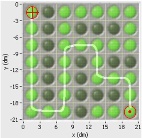
Figure 3.3 – Grid-Based Map representation. The cross marks the starting point while the dot marks the goal. ... 30
Figure 3.4 – Diagram representation of the map in Figure 3.3, containing the actions available at each cell. ... 34
Figure 3.5 – Diagram demonstrating how the Trajectory Smoother works. ... 36
Figure 3.6 – Result of the combination of the Path Planner and Trajectory Smoother, from the situation in Figure 3.3. ... 37
Figure 3.7 – Result of the combination of the Path Planner and Trajectory Smoother, using a more complex map. ... 38
Figure 4.1 – Raw measurements between and ... 43
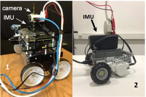
Figure 4.2 – Photos of the used MRs. 1 – MR1, Pitsco 4-wheeled robot; 2 – MR2, Lego NXT Mindstorm, 2-wheeled robot. ... 47
Figure 4.3 – MR1's Actual Trajectory. ... 49
Figure 4.4 – MR1's Position and Direction. ... 50
Figure 4.5 –Comparison between the “actual” position and the estimated position. ... 51
Figure Index
XV
Figure 4.7 –Comparison between the “actual” position and the estimated position. ... 53
Figure 4.8 –Comparison between the “actual” position and direction and the estimated position and direction. ... 53
Figure 4.9 –Comparison between the “actual” position and the estimated position. ... 54
Figure 4.10 – Comparison between the “actual” position and direction and the estimated position and direction. ... 55
Figure 4.11 – Comparison between the Data Fusion based on Velocity and on Estimation. ... 56
Figure 4.12 –MR2’s expected Trajectory 1, with the actual positions. ... 57
Figure 4.13 –MR2’s Expected Trajectory 2, with the actual positions. ... 57
Figure 4.14 –Comparison between the “actual” position and the estimated position. ... 58
Figure 4.15 –Comparison between the “actual” position and direction and the estimated position and direction. ... 58
Figure 4.16 –Comparison between the “actual” position and the estimated position. ... 59
Figure 4.17 –Comparison between the “actual” position and direction and the estimated position and direction. ... 60
Figure 5.1 – Controlled System. ... 65
Figure 5.2 – Controlled System with State variance adapter ... 66
Figure 5.3 – Controlled System with integral effect, capable of following the reference signal. 68 Figure 5.4 – Controlled System with a series gain, capable of following the reference signal. .. 69
Figure 5.5 – Controlled System, following the reference signal. ... 70
Figure 5.6 – Comparison between controlled systems, with and without variance adaptation. .. 71
Figure Index
XVI
Figure 5.8 – Variance of the estimated state, with and without variance adaptation. ... 72
Figure 5.9 – Comparison between controlled signals, with and without variance adaptation. ... 72
Figure 5.10 – Controlled System, following the reference signal. ... 74
Figure 5.11 – Controlled System used on Simulation Example 1 and 2, following the reference signal, on the interval 90s – 140s. ... 74
Figure 5.12 – Variance of the estimated state. ... 75
Figure 5.13 – Comparison between controlled systems, with and without variance adaptation. 75 Figure 5.14 – Comparison between controlled systems, with and without variance adaptation, and respective control signal, on the interval 90s – 140s. ... 76
Figure 5.15 – Comparison between controlled systems, with and without variance adaptation. 76 Figure 5.16 – Comparison between controlled systems, with and without variance adaptation, on the interval 90s – 140s. ... 77
Figure 5.17 – Variance of the estimated state, with and without variance adaptation. ... 77
Figure 5.18 – Inverted Pendulum, basic scheme used. ... 78
Figure 5.19 – Controlled System following the reference signal. ... 81
Figure 5.20 – Variance of the estimated state. ... 82
Figure 5.21 – Comparison between controlled systems, with and without variance adaptation. 82 Figure 5.22 – Comparison between controlled systems, with and without variance adaptation, on the interval 90s – 140s. ... 83
Figure 5.23 – Comparison between controlled systems, with and without variance adaptation. 83 Figure 5.24 – Comparison between controlled systems, with and without variance adaptation, on the interval 90s – 140s. ... 84
Figure Index
XVII
Figure 5.26 – Controlled System following the reference signal. ... 85
Figure 5.27 – Controlled System following the reference signal, on the interval 90s – 140s. .... 86
Figure 5.28 –Controlled systems (Cart’s position), with different variance factors. ... 86
Figure 5.29 –Controlled systems (Pendulum’s angle), with different variance factors. ... 87
Figure 5.30 – Comparison between controlled systems, with different variance factors. ... 88
Figure 5.31 – Comparison between controlled systems, with different variance factors, on the interval 90s – 140s. ... 88
Figure 5.32 –Comparison between the controlled system’s Variance and Control signals, with
different variance factors. ... 89
Figure 5.33 –Controlled System’s Control Signal, with different variance factors. ... 89
Figure 5.34 – Mobile Robot used Lego NXT Mindstorm, 2 wheeled robot, with an IMU sensor mounted. ... 90
Figure 5.35 – Sequence of Set point Trajectory. Each objective has a red or green circle limiting the objectives area. Once the MR reaches that area, the current objective is replaced by the next one. ... 92
Figure 5.36 – Time variant Trajectory. ... 93
Figure 5.37 – Comparing Position variant Trajectory and Time variant trajectory. ... 93
Figure 5.38 – Comparison between controlled MR, with and without variance adaptation, in response to a step. ... 95
Figure 5.39 – Comparison between controlled MR, with and without variance adaptation, in response to a step. ... 96
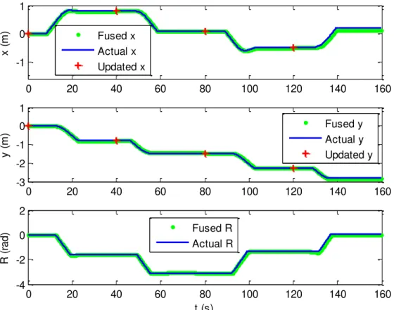
Figure 5.40 – Comparison between controlled MR, with and without variance adaptation, and Expected Trajectory. ... 97
Figure Index
XVIII
Figure 5.42 – Comparison between Control Signals applied on the MR, with and without variance adaptation. ... 98
Figure 5.43 – Comparison between controlled MR, with different variance factors. ... 99
Figure 5.44 – Comparison between controlled MR’s position , with different variance factors. ... 100
Figure 5.45 –Comparison between controlled MR’s position , with different variance factors. ... 100
Figure 5.46 –Comparison between controlled MR’s orientation , with different variance factors. ... 101
Figure 5.47 – Comparison between Control Signals applied on the MR, with different variance factors. ... 101
Figure 5.48 – Comparison between controlled MR, with and without variance adaptation. .... 103
Figure 5.49 – Comparison between controlled MR, with and without variance adaptation. .... 103
Figure 5.50 – Comparison between controlled MR, with different variance factors. ... 104
Figure 5.51 –Comparison between controlled MR’s position , with different variance factors. ... 104
Figure 5.52 –Comparison between controlled MR’s position , with different variance factors. ... 105
Figure 5.53 –Comparison between controlled MR’s orientation , with different variance factors. ... 105
Table Index
XIX
Table Index
Table 2.1 – Obstacle limit detection. ... 16
Table 2.2 – Distances from the obstacle and related angles. ... 19
List of Abbreviations and Symbols
XXI
List of Abbreviations and Symbols
Abbreviations
AMR Autonomous Mobile Robot
A* A Star algorithm
DP Dynamic Programming
EKF Extended Kalman Filter
IMU Inertial Measurement Unit
KF Kalman Filter
LQR Linear Quadratic Regulator
MC Monte Carlo
MR Mobile Robot
RL Reinforcement Learning
SLAM Simultaneous Localization And Mapping
TD Temporal Difference
UGV Unmanned Ground Vehicle
US Sensor Ultrasonic Sensor
Variables
Half of the Ultrasonic Sensor’s rotation angle [ ]
Step-size Parameter
Pendulum’s angle [ ]
State Variance at instant
List of Abbreviations and Symbols
XXII
Probabilistic Selection Parameter
Discount Parameter
Decay-rate Parameter
Observing Distance
Policy Function
Noise Correlation Matrix between instants and
Transition Matrix from to
Jacobian of function
Jacobian of function
Time increment between and
Available Action or Event taken at iteration
Model’s Dynamic Matrix
System Dynamics Matrix at instant
Model’s Expanded Dynamic Matrix
Plant’s Dynamic Matrix
Cart’s Friction Coefficient
Model Dynamic’s Input Matrix
Model Expanded Dynamic’s Input Matrix
Plant Dynamic’s Input Matrix
Speed of Sound [ ]
Model Dynamic’s Output Matrix
Plant Dynamic’s Output Matrix
Model Dynamic’s direct Throughput Matrix
List of Abbreviations and Symbols
XXIII
Plant Dynamic’s direct Throughput Matrix
Distance between the side limit of the acoustic cone and its center [ ]
Distance between the acoustic cone’s point of origin and Obstacle [ ]
Distance between the side limit of the acoustic cone and its center [ ]
Distance between the acoustic cone’s point of origin and the US Sensor [ ] Eligibility Trace at state
Function describing the vehicle’s Kinematics
Horizontal Force applied to the Cart [ ]
Gravity Constant [ ]
Function describing the expected Observations
Measurement Matrix correspondent to the th measurement at instant ( )
Measurement Matrix correspondent to the instant to th measurement ( ), estimated from
Measurement Matrices Collections between the instants and
Pendulum’s Mass Inertia [ ]
LQR’s Cost Function
Instant or Iteration
Moving Distance
LQR Controller Gain
Expanded LQR Controller Gain
Kalman Gain at instant
Set point Matrix
Pendulum’s Length [ ]
List of Abbreviations and Symbols
XXIV Landmarks Estimate States at instant
Pendulum’s mass [ ]
Cart’s Mass [ ]
Horizontal Forces applied by the Pendulum to the Cart [ ]
Covariance Matrix at instant
Covariance Matrix of the Landmarks at instant
Covariance Matrix between the Robot’s State and Landmarks at instant
Covariance Matrix of the Robot’s State at instant Vertical Forces applied by the Pendulum to the Cart [ ]
State Noise Covariance Matrix of the continuous system at instant
State Noise Covariance Matrix of the measurements between the instants and
Expanded LQR’s State weight Matrix
Covariance of the State disturbance
LQR’s State weight Matrix Output’s Set point
Robot’s Orientation [ ]
Output weight Matrix affected by State Variance
LQR’s Expanded weight Matrix
Measurement Noise Covariance Matrix of the measurements between the instants and
LQR’s Output weight Matrix Reward Function
Current Position State
Position State at iteration
List of Abbreviations and Symbols
XXV
Sampling instant at iteration
Room Temperature [
Control Vector at instant
Variance Factor
Zero mean Gaussian Measurement noise from measurement at instant
Robot’s Rotation Speed [ ]
Robot’s Forward Speed [
Value Function array
Value Function
Zero mean Gaussian Observation error at instant
Estimated zero mean Gaussian State noise from instant to
Zero mean Gaussian State disturbance at instant
Robot or Cart’s Horizontal Position [ ]
Continuous System’s State at instant
Robot or Plant State at instant
Robot or Plant Estimated State at instant
Robot’s Vertical Position [
Plant’s Output
Estimated Plant’s Output
measurement provided by the sensor at instant
Measurements Collection between the instants and
Measurement provided by the th sensor at instant
1 Introduction
1
1
Introduction
1.1
Motivation
Everyday life incorporates an increasing number of intelligent machines capable of performing complex and diversified tasks. Purchases and sales, bank transactions, doubt clarification, or driving support, are examples of activities executed by such machines.
In what regards autonomous mobile platforms, these are often found in industrial environments, performing transport functions of materials or components. However, there are areas where the use of automatic machines is still incipient. One example is the execution of tasks requiring mobility in humanized environments. The use of Mobile Robots (MR) to perform autonomous tasks in offices, commercial areas, or even in households, is still at an early stage.
A reason for this fact may be attributed to present technological limitations. Homes or offices are less structured than factories, and are subjected to frequent changes. In particular, the available area for movement and position of objects undergoes frequent alterations. On the other hand, the installed infrastructure is very different from the manufacturing environment:
Specific support elements for the mobile robot’s localization and movement (beacons,
sensors, etc.) are in small number or non-existent;
Also the way humans relate themselves with the Unmanned Ground Vehicles (UGVs) is distinct. On a manufacturing plant moving machines are provided priority, while in an office or commercial space, humans always have priority.
This reality creates specific requirements to UGV development.
This dissertation addresses the development of an autonomous mobile platform capable of moving between different points of an environment with a (map) structure which is just partially known and suffers changes along the time. It is assumed that the tasks associated to localization and displacement of the mobile unit should be performed almost exclusively based on the sensor capabilities installed onboard.
1 Introduction
2
Figure 1.1 – Interdependency scheme of the subjects approached in this work.
1.2
Problem Formulation
What does a mobile robot need to be autonomous?
For a person to be able to give the first step it requires seeing where he (she) wants to go or, more importantly, where that first step is to be placed. Following this idea, before a mobile structure should start to move it is required to analyze the surrounding environment. Sensors, can either be located on the mobile structure or external to it, are what gives the robot the perception of its environment.
To have a better grasp of the mobile robot’s surrounding environment, the information from the different sensors must be combined and integrated with the knowledge already available. The data provided by sensors may be used, for example, to update the environment information by adding new obstacles or removing obstacles no longer detected.
11.2 Problem Formulation
3
To implement a Task, like moving from one point to another, it is not enough just to order it. The robot movement is subjected to disturbances and uncertainties so its displacement must be done in a controlled way. This usually requires additional sensing information on the MR’s
location and movement.
This set of abilities has to be integrated by means of a supervising system capable of coordinating them harmoniously with the purpose of concluding its missions.
This dissertation addresses several of the elements afore mentioned. It is aimed to evaluate problems associated to the different subjects as well as the technical solutions. Due to this widespread nature the degree of attention dedicated to each subject is varied.
To gather relevant data from its environment the robot uses sensors. Both the sensors and the type of data provided are diversified: cameras provide images that need to be analyzed for extraction of features; long range obstacle detectors, like laser sensors and ultrasonic sensors, can give the distance to obstacle that are within line of sight; touch sensors detect obstacles when the robot gets in direct contact with them.
Whatever the type of sensor, the data provided must be analyzed to produce relevant information. The effort required to perform this analysis varies with the type of data, so the resources needed are different depending on the sensors installed on the robot.
One of the Mobile Platforms used for this work carries an Ultrasonic Sensor. One of the subjects addressed by the dissertation is the use of the Ultrasonic Sensor to detect obstacles, and to determine its location (distance and direction).
To plan a robot’s route towards a goal position requires the use of a map, identifying the
obstacles and the free paths. Humans create mental maps almost unwarily, that is not the case of an Autonomous Mobile Robot (AMR), where sensor measurements must be processed, giving
raise to a map of the working environment. Maps besides being used to plan the UGV’s path,
can also help to determine the location within the working area. This subject is usually named by Simultaneous Localization And Mapping (SLAM), that is also discussed in this dissertation. The dissertation also deals with the problem of using existing map information to plan the robot trajectory over the free space within the working area.
11.2 Problem Formulation
4
as, inertial information and odometry are some of the more frequently used methods to
determine the MR’s position. Each of these approaches relies on its own type of sensors. It is possible to combine the information from several sensors, giving different types of data, to provide a better knowledge of the surrounding environment and improve the precision of the robot location. This subject is covered within the sensor fusion framework.
An UGV also needs a trajectory controller to allow it to follow the predefined trajectory. While it is following the trajectory, the UGV may be subjected to disturbances of different nature that may lead it off track. The trajectory controller’s purpose is to compensate for disturbances and ensure an adequate tracking of the planned trajectory. The controller’s performance is strongly connected to the ability to determine the robot movement attributes (such as position, speed, and orientation).
An important controller feature is the ability to comply with different degrees of precision from the movement attributes data. The Mobile Platform’s controller needs to be able to tolerate
some degree of error and to adapt the speed accordingly. In this dissertation an approach for the development of such a Controller is studied.
Figure 1.2 ilustrates the hierarchical dependencies between each subject approached in this dissertation.
11.3 Contributions
5
1.3
Contributions
Development of an asynchronous sensor fusion algorithm and its integration with a
trajectory controller. This controller uses a modified version of the LQR’s algorithm. This
modification consists on the use of a cost function, that incorporates the uncertainty associated
to the robot’s movement.
A trajectory planning algorithm was developed, based on a Reinforcement Learning scheme. This algorithm was implemented as an interactive program.
An ultrasonic sensor was studied, and its use for measuring the distance to an obstacle was analyzed.
A small autonomous robot was implemented. The robot is able to able perform a predefined trajectory without the help from external sensors or beacons.
1.4
Dissertation Overview
The dissertation is organized with the following structure.
The first chapter introduces the Motivation for the Dissertation’s subject and presents the
Problems that will be covered. The dissertation structure is also presented.
Chapter 2 addresses the study of Obstacle perception sensors, focusing on the Ultrasonic Sensor (US). It presents the basic functions of US sensors. It studies the sensor’s sensing Area,
that is, the sensing cone width and the relation between the true and the computed distance. Attempts are made to obtain the position and profile of the obstacles within the sensor’s range.
Throughout this chapter the problems encountered are also depicted.
11.4 Dissertation Overview
6
Occupancy grid-based map is used to compute the robot’s trajectory, from the original position to its desired destination.
Chapter 4 deals with the problem of finding the mobile Platform’s Localization, using only its own on-board sensors. It is assumed that each sensor has its own independent sample rate, although the sensor’s sampling may be asynchronous. As an example, the delay associated with processing image information is usually random. Experiments are presented using two different Mobile Platforms, and the estimation of the platforms’ position is made in a number of different fusion situations.
Chapter 5 addresses the development of a controller for the AMR. The planned controller is a Linear Quadratic Regulator (LQR) based adaptive speed regulator depending on the uncertainty of the robot’s state. This controller is applied to one of the MR’s, mentioned on the second part of Chapter 3, to follow a pre-planned trajectory.
Chapter 6 summarizes the results drawn from the work developed for the dissertation. It also proposes a set of research topics to be developed within this line of work.
2 Environment Perception
–
Ultrasonic Sensor
7
2
Environment Perception
–
Ultrasonic Sensor
An AMR requires sensing capabilities in order to avoid collision with static or moving obstacle. A number of sensors using different technologies exist for this purpose, such as lasers, infrared detectors and contact switches.
This chapter addresses the study of an Ultrasonic Sensor, its features and the ability to detect and evaluate the obstacle position.
2.1
The Ultrasonic Sensor for distance measurements
Ultrasonic sensors may be categorized as active sonars with monostatic operation. In other words, it emits sound pulses and receives the echoed signal. The sonar calculates obstacle’s
distance using the time interval between the signal emission and reception, as the distance is proportional to the time, knowing the speed of the traveled sound. Ultrasonic (US) sensors generate high frequency sound waves that are above the human hearing range ( - ).
Sonar is one of the most frequently used type of sensors for obstacle detection, mostly because they are cheap, easy to operate and make no physical contact, resulting no wear due to friction, and it doesn’t alter the environment.
Ultrasonic sensors don’t only carry the functionality of obstacle detection and avoidance.
They are also used for localization and navigation. Figure 2.1 presents the mobile robot
platform and a it’s ultrasonic sensor mounted on a rotating servo.
2.1 The Ultrasonic Sensor
8
Figure 2.1 –NI Robotics Starter Kit
Figure 2.2 – Example of the sound reflection produced by the sensor. It shows two examples of obstacle detection (a and b), and an example of obstacle’s misdetection (c).
The main problems with US Sensors, commonly mentioned by various authors [Cardin07; Ayteki10; Borens88], are:
When the sound emitted by the sensor hits an obstacle’s surface, it works almost like a
light beam hitting a mirror surface. If the surface is perpendicular to the emitted signal, then it goes straight back to the sensor. However, the surfaces encountered aren’t always parallel to the sensor, meaning, the obstacles aren’t always detected, as the sound may be
reflected away from the sensor (Figure 2.2.(c)).
The signal emitted by the US sensor is in a form of an arch (acoustic cone), which gives the possibility that the obstacle detected might not be located right in front of the sensor. There might even be more than one obstacle at range and only the closest be detected (Figure 2.3).
a)
b)
2.1 The Ultrasonic Sensor
9
Figure 2.3 –Ultrasonic Sensor’s acoustic cone, with a angle of detection.
2.2
Ultrasonic Sensor Features
The ultrasonic sensor used in this work is a Parallax Ping)))™ Ultrasonic Distance Sensor.
According to the sensor’s datasheet [Ping13a; Ping13b], it can detect obstacles from up to
, as well as measure the distance at which the obstacle is located. The acoustic cone has an angle of 40 (20 for each side Figure 2.3).
Although these features are indicated by the manufacturers, it is still necessary to verify them with a few tests.
2.2.1
Width of the Ultrasonic Sensor’s Acoustic Cone
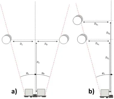
The ultrasonic sensor emits a sound, and during the journey from the sensor to the obstacle and back to the sensor, the sound disperses almost in a form of a cone (acoustic cone), as it loses energy (intensity). Any obstacle(s) located inside this cone may reflect the sound back to the sensor, allowing the sensor to compute the distance to the target, but not the position within the cone. To have a notion of the sensor’s sensing cone, it is required to know the Sensing Angle ( ), the angle of detection, and the distance between the sensor and the origin of the cone ( ).
2.2 Ultrasonic Sensor Features
10
placed over a parallel line to the sensor, located at a distance from the sensor. The obstacle
starting position is located outside of the sensor’s detection range.
The target is moved over the parallel line to the sensor, and the region where detection occurs is registered. The sensor detects the obstacle from a distance of ( ) to the left of the center until ( ) to the right.
Figure 2.4 - Representation of the experiment performed to obtain the angles of the acoustic cone.
The procedure was repeated at a different distance from the sensor. With the target placed at ( ) the range of the obstacle detection is between ( ) to the left and
( ) to the right.
(2.1)
(2.2)
(2.3)
From these measurements the angles of detection ( and ) were computed, resulting in
and , respectively. The total detection angle of the used sensor was about (
2.2 Ultrasonic Sensor Features
11
+ ), but knowing the acoustic cone’s angular width isn’t enough, it is required to know how far is actually the point of origin ( , distance between the obstacle and the sensor’s parallel
line), as it is not at the same distance as is the distance to the sensor, . The average distance
is from the sensor to the point of origin to the sensor. Knowing this angle can allow for a more precise location the obstacles, or to delimit the obstacles geometry.
2.2.2
Ultrasonic Sensor’s Measurement R
eadings
The second experiment aims to assess the accuracy of the distances to target, measured by the sensor. For this purpose it an obstacle with a flat surface (turned to the sensor) positioned around the central position is used. The test consists on placing the obstacle as far as possible from the sensor and recording the true distance and the measure provided by the sensor. The target is then moved closer to the sensor and new measures are obtained. This procedure is repeated several times until the obstacle gets as close as from the sensor. The collected data is used to compare the sensor measures with the true distances and to compute any necessary corrective actions (gain or off-set error correction) and to evaluate the consistency of results.
At the beginning of this experiment, it was noticed that the sensor was providing incorrect values, indicating that the target was far closer than it really was. As an example, with the obstacle at , the sensor presented measured values between and . This error occurs systematically. The explanation for this problem appears to be related with echoes occurring within a closed environment. The generated sound has enough intensity so that, after being reflected, it reaches another obstacle, from which it bounces back returning to the US sensor and confusing it. During the experiments, the echo was from the wall behind the robot or the robot itself (Figure 2.5).
Following equation (2.4), with the room temperature ( ) about , the speed of sound, during the experiment, was .
(2.4)
According to the data sheet [Ping13a; Ping13b], the burst of pulses can be detected from
2.2 Ultrasonic Sensor Features
12
burst of sound took longer than to reach back to the sensor, it could confuse the sensor by making it think the obstacle is at a few centimeters away, by associating the sound burst to the next cycle.
In the present situation, the echo from the wall, which was about , took about ,
longer than the maximum detection time, with the obstacle at (total distance traveled by the sound was ). When the echoed sound reaches the sensor, it assumes the obstacle is closer than it is.
As the sensor does not allow the intensity of the generated sound to be adjusted, it was not possible to reduce the intensity of the produced sound.
The same experiment was performed with the obstacle covered by a sound absorbing material, such as cloth. This has an effect similar to reducing the sound intensity and allows the sensor to provide adequate measures. Measures were recorded with the covered obstacle positioned at distances ranging from down to away from the sensor. The results are summarized on the graph from Figure 2.6. All the measurements provided by the sensor had an average value that is larger than the actual distance.
2.2 Ultrasonic Sensor Features
13
Figure 2.6 – Relationship of the measurement provided by the sensor and the actual value. The measurements are the distances between the detected obstacle and the sensor.
2.3
Target Detection
2.3.1
Use a Rotating Ultrasonic Sensor
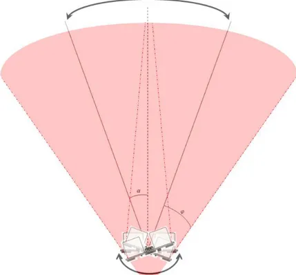
On another experiment the ultrasonic sensor was rotated (Figure 2.7 and Figure 2.8), to
evaluate the obstacle’s profile obtained from using a rotating sensor. As the rotation axis is not
placed at a symmetry axis of the sensor geometry, the rotation produces an asymmetry when comparing the readings. The readings obtained when scanning from left to right are not the same as the readings scanned from right to left. This variation can also be seen as another problem that isn’t mention by many authors.
The results of this test are presented on the Figure 2.9, which shows the temporal progress of the measured distance by the sensor, as with its angular position. The Target used has a flat surface, wide, positioned about away from the sensor, parallel and centered to
0 0.2 0.4 0.6 0.8 1 1.2 1.4 1.6 1.8
0 0.2 0.4 0.6 0.8 1 1.2 1.4 1.6 1.8
Real Measurement (m)
2.3 Target Detection
14
it.The sensor turns with a speed of , within a range . The target surface was covered with a sound absorbing cover to reduce the burst intensity emitted by the sensor.
The test results are summarized on the graphs from Figure 2.10 to Figure 2.13. The first graph (Figure 2.10) shows the measured distance as a function of the rotation angle. As expected it may be noticed a slight increase of the distance towards the edges of the surface. From the information used to produce Figure 2.9, the instant when the obstacle’s limit was detected and the corresponding sensor’s orientation, were extracted. This information was assembled on the
Table 2.1 is divided between the reading made from right to left and the readings made from left to right. As the table shows, there is a significant difference between the detected angles.
The second graph plots (Figure 2.11) the target surface on a plane. The average distance, provided by the sensor is . Without taking into account the limits of the
sensor’s acoustic cone, the obstacle is seen as having an average width of .
At this distance, according to the equations presented (2.1) to (2.3), the sonar cone, obtained
with the round tubular target, has a width of , wider than this new target estimated width. This shows that the obstacle surface geometry is very important as it affects the measures produced by the sensor. A round surface obstacle, such as a tube, has the capability to reflect the burst of sound back to the sensor, wherever it is located within the acoustic cone. Flat surface obstacles are different, because of their relative orientation to the sensor affects the detection. The obstacle angle may either allow it to be seen, by reflecting the signal back to the sensor, or not seen, by reflecting the signal away from the sensor. The echoes resulting from secondary reflections on other obstacles also contribute to confuse the sensor measurements. A more extensive research on this subject is required, which is beyond the scope of this document.
The results of this experiment are also shown in Figure 2.12, which separates the measurements read by the sensor from Right to Left from the ones made from Left to Right. The measurements read by the sensor from Left to Right are presented in Figure 2.13. There is a
difference of the detected obstacle’s position between the readings made from Left to Right and
2.3 Target Detection
15
Figure 2.7 –Scheme of the Sensor’s Roratory axis. Its total rotating angle is .
2.3 Target Detection
16
Figure 2.9 – Results obtained from the Rotating US Sensor. The top graph presents the measured value. The second graph shows the Sensor’s orientation over Time.
Table 2.1 – Obstacle limit detection.
Right to Left Left to Right
Right side of the
obstacle Left side of the obstacle Left side of the obstacle Right side of the obstacle Time ( ) Angle ( ) Time ( ) Angle ( ) Time ( ) Angle ( ) Time ( ) Angle ( )
Mean Mean Mean Mean
15.11
Obstacle’s detection
Angle width ( ) Obstacle’s detection Angle width ()
0 2 4 6 8 10 12 14 16 18 20
0 1 2 3 4 M e a s u re m e n ts ( m )
0 2 4 6 8 10 12 14 16 18 20
2.3 Target Detection
17
Figure 2.10 – Readings obtained by the sensor, highlighting the detected obstacle. Measurements between the Obstacle and the Sensor over Time. This data is the same as in the Figure 2.9.
Figure 2.11 – Position of the detected obstacle on a plane.Same information as the one used in Figure 2.10.
-250 -20 -15 -10 -5 0 5 10 15 20 25 0.5 1 1.5 2 2.5 3 3.5 M e a s u re m e n ts ( m ) Angle (Deg) No obstacle detected Obstacle detected
-1.50 -1 -0.5 0 0.5 1 1.5
0.5 1 1.5 2 2.5 3 3.5 y ( m ) x (m)
2.3 Target Detection
18
Figure 2.12 – Position of the detected obstacle on a plane, identifying with only readings from Right to Left. Same information as the one used in Figure 2.11.
Figure 2.13 – Position of the detected obstacle on a plane, identifying with only readings from Left to Right. Same information as the one used in Figure 2.11.
-1.50 -1 -0.5 0 0.5 1 1.5
0.5 1 1.5 2 2.5 3 3.5
y
(
m
)
x (m)
No obstacle detected Obstacle detected
-1.50 -1 -0.5 0 0.5 1 1.5
0.5 1 1.5 2 2.5 3 3.5
y
(
m
)
x (m)
2.3 Target Detection
19
2.3.2
Other ways to detect a Flat Surfaced Target
On the previous experiments, for the sensor to provide correct measurements, the obstacle had to have a sound absorbing surface, to avoid echoes. The next results are obtained with an uncovered flat obstacle (no sound absorbing surface). However, to avoid the echo the obstacle cannot be perfectly parallel to the US sensor. Echo effect is avoided by rotating the obstacle by a few degrees. This way, secondary sound reflections are avoided.
It is verified that the closer the obstacle is to the sensor, the larger the angle of the obstacles needs to be. This can be verified from the data from Table 2.2, which presents the distances the
obstacle was positioned and the angle it was adjusted in relation with the sensor. The angle indicated was the minimal angle found so the sensor could detect the obstacle.
Table 2.2 – Distances from the obstacle and related angles. Obstacle’s Distance ( ) Obstacle’s Angle ( )
2.4
Summary
This chapter addressed the study of the Ultrasonic Sensor installed on the National Instruments mobile robot, its characterization and the evaluation of the problems on detection of
different obstacles.
A comparison between the sensor’s reading and the actual distance was made, showing that
it possessed an average offset of .
An experiment was made to verify the sensor’s sensing width, which demonstrated the sensor had a sensing angle of about , close to what the datasheet indicated ( ).
2.4 Summary
20 decrease of the sensor’s detection range. With a different sensor it would be interesting to study the development of an adaptive scheme to avoid echo, but still keep the detection range.
Under controlled conditions it is possible to cover all the obstacles with sound absorbing material, as it was done for the experiments. The use of an autonomous MR within an unknown environment where unpredictable obstacles may be encountered, such as in an office, makes this solution unfeasible.
3 Mapping and Trajectory Planning
21
3
Mapping and Trajectory Planning
This chapter addresses the problem of map construction and its use for trajectory planning. It describes the use of the algorithm EKF-SLAM to associate the robot with the various detected landmarks on the environment. An algorithm, based on reinforcement decision making, is developed for the planning of the mobile robot’s trajectory.
3.1
Environment Mapping
Maps are an important element for planning and control of AMR Movement. They allow to plan the sequence of actions to be performed by the robot, to verify the robot’s actual position
and to make necessary corrections to the robot’s performance.
The construction of a map requires the environment’s geometry and the obstacle positions within the environment to be perfectly known [Thrun05]. However, this is not the kind of environment in which humans live:
Generally speaking, there is no complete or exact information about the surrounding environment;
The surrounding environment is subject to changes.
These motives make the robot mapping an important subject in association with AMR, as well as a pointer for research. The basic goal is to build a map (mostly 2D/3D) of the surrounding environment, detecting walls, furniture and other obstacles, and it may also be used
to determine the observer’s (robot) position and orientation to plan trajectories to take [Thrun05; Durant06; Valenc13].
An UGV may locate its position through one of two types of mechanisms:
Idiothetic – uses a combination of models and sensors, like IMUs, to estimate the
Mobile Unit’s position by dead reckoning. This means it tends to accumulate error. Allothetic – uses external information to locate itself, such as landmarks, by
triangulating its position. This approach tends to present constant error, depending on
3.1 Environment Mapping
22
To build a map of the environment through the robot’s sensorial information requires the knowledge of robot’s position and the estimation of the obstacles position. This means that the mapped obstacle positions depend on the robot’s own position, giving rise to a correlation between the obstacles’ and the robot’s position errors [Thrun05, Riisga05, Namins13].
On the other hand, to locate the robot’s position using the map, it is necessary to know which
obstacles and landmarks are within the robot’s range. The detected landmarks need to be already registered on the map, so that the mobile platform may be able to locate itself. In this case the robot’s position depends on the position of the obstacles around it [Thrun05].
The acronym SLAM stands for Simultaneous Localization And Mapping. It is a set of techniques for mapping within the autonomous mobile platforms framework. It combines localization techniques with mapping, both computations being performed simultaneously.
SLAM is a “chicken-or-egg” type of problem – a map is needed for localization, and localization is required for mapping.
3.1.1
Mapping and Localization of the Robot
When the robot moves, that is, it obtains a new position, and it updates its estimated position through odometry computation. On this new position, the robot extracts the landmarks and attempts to associate these to the landmarks that it has previously seen. The re-observed landmarks are used to update the robot’s position, while the new ones are added to the map.
The basic algorithm is composed by the following steps:
1. Update the current state estimate using the odometry data. 2. Update the estimated state from re-observing landmarks. 3. Add new landmarks to the current state.
These steps are considered on the Figure 3.1. The first step involves the odometry
information, and the robot’s state. This state usually contains the robot’s position, which
3.1 Environment Mapping
23
The second step uses the robot’s position estimation to identify the landmarks and their configuration relative to the robot. The actual position (or an approximation) is determined and updated from these landmark configurations.
This step also includes the landmark’s position uncertainty update, for every known landmark.
The third step adds the newly detected landmarks to the map using the robot’s corrected
position.
Figure 3.1 –Example of the UGV’s SLAM process.
1 –UGV’s estimated performance;
3.1 Environment Mapping
24
3.1.2
Some Considerations about Landmarks
Landmarks should be re-observable by allowing the detection from different positions and angles. They should also be unique enough so they can be easily identified or distinguished from each other, so there might not be a mix-up when re-observing them.
Figure 3.2 – Example of wrong Data Association Problem.
This problem is related with Data Association. Figure 3.2 represents an occurrence of wrong Data Association. The UGV has three landmarks in its Environment Model and it only detects two of them. The robot can either be found in the situation a) or in the situation b). This kind of
problem can cause the mapping system to diverge, with catastrophic consequences [Durant06].
Another important point about mapping is that landmarks should not be too far apart, because the MR will accumulate error from the odometry by itself, leading to larger error on the position of the new landmarks detected. In other words, the mapped environment needs to have, at least, a trail of landmarks so the robot will have a good performance, and also be capable to avoid getting lost.
The robot also needs to be able to distinguish stationary obstacles, such as walls and furniture, from moving obstacles, such as people or other mobile robots. When (almost) stationary obstacles are moved or altered, this must be detected and the map adjusted accordingly.
3.1 Environment Mapping
25
3.1.3
EKF-SLAM Algorithm
The EKF-SLAM is one of the most commonly used Mapping algorithms. As the name implies, it uses an Extended Kalman Filter (EKF) to associate the robot with the various detected landmarks on the environment. This algorithm tends to be used on the detection of
features of the environment, through the robot’s sensorial perception. These features are used to
identify landmarks, so they will also be used for localization purposes. The EKF-SLAM is divided into two parts: the motion update, where an estimate of the AMR’s position is
computed; and the correction update, where the robot’s position estimate, as well as the
landmarks’, are corrected [Durant06; Skrzyp09; Namins13; Riisga05].
On the EKF-SLAM method, the vehicle’s state transition (or motion) is described by the expression
(3.1)
where is the function describing the vehicle’s kinematics, is the control signals applied and is the state’s zero mean uncorrelated white noise. The description of the observation model is done in the form
(3.2)
where is the function that estimates the expected readings from the environment, is the detected landmarks states and is the observations’ zero mean uncorrelated white observation noise. This noise is also assumed to be uncorrelated with .
The estimation update is described in the following form
(3.3)
(3.4)
(3.5)
3.1 Environment Mapping
26
where is the Jacobian of evaluated at the estimate . and are, respectively, the covariance matrix on the vehicle’s state and on the map. is the covariance matrix between the vehicle’s state, , and all landmarks, . is the covariance of .
At this point, the main concern is the estimation of the robot’s position. Its “uncertainty”, , affects the cross term . The map’s covariance, , remains unchanged.
The correction-update step is performed according to
(3.7)
(3.8)
where
(3.9)
(3.10)
(3.11)
being the Jacobian of evaluated at the estimate and . is the innovation covariance, used to compute the Kalman gain matrix, , and , is the covariance of .
At this point the robot’s poses (position and orientation) are corrected through the use of the observations made and their expected values, . Also, the landmarks’
positions are corrected (3.7). All of the covariance terms are updated by the equation (3.8), including the covariance between all stored landmarks, , (3.11). At this step the landmark’s accuracy is improved through the use of observation data (3.9) and(3.10).
3.1 Environment Mapping
27 environment’s disturbances. Due to the uncorrelated nature of the noise, the respective noise covariance matrices have a diagonal structure.
3.1.4
An alternative Algorithm
Another commonly used mapping algorithm is FastSLAM [Durant06; Bailey06; Kurt12; Calond06]. It uses a Rao-Blackwellised particle filter to perform the landmark association. It has several advantages over the EKF-SLAM, such as its robustness against ambiguous data association. It deals with this problem by replacing the wrong association with a re-sampled one. It also provides a lower estimation error, compared with the EKF-SLAM, although it presents less consistency. This inconsistency can cause trouble by leading to the filter’s divergence.
3.2
Trajectory Planning
For an AMR to move around it requires a controller and a supervising system. It also needs to know its location within the surrounding environment, for which it requires a map. To know how to get from one location to another it is necessary to define a set of positions to be reached and actions to be performed. This leads to the question: How can a robot decide on the actions to perform to complete the mission? [Aranib04]
One of the required tools is Path Planning, or motion planning, which addresses the problem
of setting up the robot’s movement in a 2D or 3D world, which contains obstacles. The
objective of this kind of planning is to determine what actions are appropriate for the robot to perform, so it can reach the envisaged state, while avoiding collision with the obstacles, among other mechanical limitations.
The essence of making such decisions can have both immediate and long term effects. The best choice to make depends on future situations and how they will be faced.
3.2 Trajectory Planning
28
Various path decisions making algorithms exist, such as RRTs (Rapidly-Exploring Random
Trees) [Bruce02; LaValle98], A* (A Star) [Hart68], and Dijkstra’s algorithm [Dijkst59].
In this work, such decisions are made through a Reinforcement Learning based algorithm, similar to what the author of [Aranib04] proposes. The idea is to allow the MR to learn the path it should take to reach the desired goal.
Assuming the MR already knows its surrounding environment, by simulating the movement throughout the map, a number of alternative paths are tested. To determine which path is the best, it counts the number of actions taken. Once the simulated MR reaches the goal, it attributes
a “suggestive” value to each position which was walked through, related to the viability of the
path.
3.2.1
Reinforcement Learning
An important question is “What is the best set of decisions to take in order to reach the desired goal?” The RL’s solution for this problem is through a set of successive experiments. From the performed experiments, the best one is chosen. The choices made are measured through rewards. An example of such way of learning is applied to animal training. If the animal performs well then it is rewarded, if it performs badly it is punished. This is also done on Reinforcement Learning through rewards and costs.
The distinguishing factor of the Reinforcement Learning is not the learning methods used, but the learning problem in hand [Sutton98].
3.2.1.1
Main Structure of Reinforcement Learning
3.2 Trajectory Planning
29
State ( ), in RL, is a representation of a set of values or conditions which the process or its model encounters. In this case, it is the robot’s position inside the mapped environment. Using a grid-based map, this division is easily made.
For a transition between states to be performed, actions or events ( ) need to take place. These actions may have been decided by the system, like the MR’s decision of turning on the
present position, or by an external agent, like a foreign presence pushing the robot to a different position. At this initial stage, no external presence is added to the problem.
The Reward Function, , defines the goal of the reinforcement learning problem. Generally speaking, it attributes a value for each state or state/action pair. That value is named a reward. It defines if the state/action taken is good or bad, for the aim of the RL system is to collect the maximum reward possible.
The Reward Function indicates how good a decision is in the short run, while the Value Function, , indicates how good a decision is on the long run. In other words, the Reward
Function indicates how much reward the system will gain if it chooses that action. The Value Function indicates the total reward the system might gain in the end if it chooses the action. Returning to the animal training example, if the animal knows it will gain a large reward, even though it will make a few misbehaviors, it will take that set of actions.
The Policy Function defines the overall behavior of the system. In other words, depending
on the system’s state, it chooses which action it should take, as a response to the stimulus. This may be as simple as a function or lookup table or so complex that it requires extensive computations, like in a search process. This is the function that defines the system’s personality.
It can be stubborn, by following the currently known best path, or curious and open minded, by walking around, looking for a better solution.
These three elements, when combined, can lead to the selection of the best sequence of actions to reach the desired goal, that is, the one yielding the largest reward.
For the System to learn how to act, it doesn’t necessarily require for the actual action to be
3.2 Trajectory Planning
30
However, the model may differ from reality, like the existence of unexpected obstacle along a planned path or some unexpected robot behavior. On these occasions, the combined use of both learning methods (simulation and practice) is certainly an advantage.
One of the challenges, when using RL, is the trade-off between exploration (search through every state and action available so it can pick the best one) and exploitation (uses what it knows to collect the best reward). It is the difference between searching the whole environment after all the existing rewards in it, wasting a lot of time, or just selecting among the already experienced state-action pair. This challenge usually reflexes on Policy Function [Sutton98].
3.2.1.2
Path planner with RL
The intention is to plan the best trajectory for the MR to take to reach the desired location. This study uses a simplistic 2D Grid Based map (Figure 3.3). Each cell is identified as a State of the system. Associated to each state there is a boolean indicating if that space is free of obstacle
or not. The MR’s trajectory has a starting point and a finishing point.
Figure 3.3 – Grid-Based Map representation.
The cross marks the starting point while the dot marks the goal.
3.2 Trajectory Planning
31 Reward Function
There is no difference between all states on the map, except for the finishing state, as it is the desired goal. As so, the transition to this goal state, , carries the highest (positive) reward. In
the present situation the value is used. The remaining states are used to reach this position. If they carry a reward value, that means there is no loss by walking around. In reality, for an UGV, there is always loss of time, energy and physical wear, among others. So it requires the attribution of a negative reward. In this situation it is attributed the reward value to the transition to any of the remaining states. The resulting Reward Function is
Reward Function
( ) // is the State in question. if( == ) // Verifies if is the State Goal, .
return ; else
return ; end;
end;
Value Function
The Value Function’s array ( ) indicates the best states for the MR to move to. These suggestions are based on the values each state posses on the array. The values, calculated by the Value Function, , depend on the MR’s present state, where it is positioned and the next state, to where it will transition to.
This function has many variations, depending on the methods used for estimating the Value Function, such as Dynamic Programming (DP), Monte Carlo (MC) and Temporal-Difference (TD) [Sutton98].
In this case a variation of the Temporal Difference Method was used, the On-line Tabular (TD( )) [Sutton98]. The TD Method is chosen over the other two methods mainly due to two features:
Using values of the successive states to estimate the value of the current one. This is called bootstrapping.