Crackle and wheeze detection in lung sound signals using convolutional neural networks

(1)

wheeze detection

in lung sound

signals using

convolutional

neural networks

Pedro Sousa Faustino

Mestrado Integrado: Engenharia de Redes e Sistemas

Informáticos

Departamento de Ciência de Computadores 2019

Orientador

(2)

O Presidente do Júri,

(3)

I thank Miguel Coimbra, Jorge Oliveira and Francesco Renna for the guidance they gave me during the thesis, for their availability and willingness to help with their insights and opinions during the work, as well as their friendliness. I also thank José Reisinho for his discussions and insights which proved to be very useful in finishing this thesis.

And finally, I thank my mom, my sister, my grandma and Tiago for all of their support and motivation to finish this thesis.

(4)

MOTIVATION: Respiratory disease is among the leading causes of death in the world. Most of these deaths occur in poorer countries where pollution is more prominent and medical care is less accessible. Prevention and early detection are essential steps in managing respiratory disease. Auscultation is an essential part of clinical examination as it is an inexpensive, noninvasive, safe, easy-to-perform, and one of the oldest diagnostic techniques used by the physician to diagnose various pulmonary diseases. The drawbacks of this procedure is that doctors require experience and ear accuity to provide a more accurate diagnosis to the patient. It is especially hard since some sounds are harder to detect because of the limitations of the human ear.

OBJECTIVES: The objective of this work is to successfully detect and/or classify crackle and wheeze sounds in the lung sound digital signal, using advanced signal processing techniques combined with convolutional neural networks.

METHODOLOGY: We utilize the ICBHI 2017 challenge dataset to test our methods, which consists of 126 participants and 6898 annotated respiratory cycles. We experiment with raw audio, Power Spectral Density, Mel Spectrogram and MFCCs as input features for a convolutional neural network. We then perform five-fold cross validation to compare the final methods.

RESULTS: Utilizing a Mel Spectrogram as the input features for a convolutional neural network showed better results than the other methods, achieving a test accuracy of 43%, an AS of 0.43, a HS of 0.42, a SP of 0.36 and a SE of 0.51.

KEYWORDS: lung, sound, signal, auscultation, automation, classification, deep, learning, convolutional, neural, network, crackle, wheeze.

(5)

MOTIVAÇÃO: A doença respiratória está entre as principais causas de morte no mundo. A maioria destas mortes ocorre em países pobres onde a poluição é mais significativa e o acesso a tratamento medicinal é menor. A prevenção e a deteção são partes essenciais do controlo da doença respiratória. A auscultação é essencial no exame clínico pois é um método de baixo custo, não invasivo, seguro, fácil de executar e um das técnicas mais antigas e usadas para o diagnóstico de doenças pulmonares. A desvantagem deste método é que os doutores precisam de experiência e acuidade auditiva para conseguirem dar um diagnóstico de melhor qualidade. Isto torna-se ainda mais difícil devido às limitações do ouvido humano.

OBJETIVOS: O objetivo deste trabalho é a deteção e classificação de crackles e wheezes em sinais digitais de som de auscultação pulmonar, utilizando métodos de processamento de sinal digital combinado com o uso de redes neurais convolucionais.

METODOLOGIA: Nós utilizamos a base de dados de som de auscultação que foi utilizado para um desafio na ICBHI 2017, para testar os nossos métodos. A base de dados foi recolhida de 126 participantes e contém 6898 ciclos respiratórios anotados. Nós experimentados com o processamento de som direto, com o Power Spectral Density do sinal, com o espectrograma de Mel do sinal e com os MFCCs do sinal como input para a rede neural convolucional. Depois comparamos os resultados finais utilizando five-fold cross validation.

RESULTADOS: A utilização do espectrograma de Mel como input para a rede neural demonstrou os melhores resultados, conseguindo uma accuracy de 43%, um AS de 0.43, um HS de 0.42, um SP de 0.36 e um SE de 0.51.

PALAVRAS-CHAVE: pulmão, som, sinal, auscultação, automação, classificação, deep, learning, rede, neural, convolucional, crackle, wheeze.

(6)

List of tables

Table 1 - Test metrics for each method in the challenge. The best results for each of the metrics

are highlighted in bold. With the mean and standard deviation for each metric. 35

Table 2 - Statistics for each of the cycle classes. 36

Table 3 - Duration statistics for all recordings and cycles. 36

Table 4 - The patient sample count, the recording sample count and the cycle sample count for

each of the equipment types. 36

Table 5 - The patient sample count, recording sample count and cycle sample count for each of

the auscultation points. 37

Table 6 - The patient sample count, recording sample count and cycle sample count for each

acquisition method. 37

Table 7 - Which equipment produces each of the sampling rates, as well as the patient sample

count, recording sample count and cycle sample count for each of the sampling frequencies. 37

Table 8 - Data distribution of the five folds. 42

Table 9 - Test results for each of the input feature types of the CNN model, using the challenge’s

data split. The best results for each of the metrics are highlighted in bold. 47

Table 10 - Five-fold cross validation mean test metrics for each method. The best results for each

(9)

List of figures

Fig. 1 - Schematic of the respiratory system displayed by the upper and lower respiratory tract

region [50]. 12

Fig. 2 - Schematic of the respiratory system showing the anatomy of the lung [51]. 13

Fig. 3 - Time-domain characteristics and spectrogram of (a) normal, (b) wheeze, and (c) crackle

lung sound cycle [7]. 17

Fig. 4 - Structure of a feed-forward ANN with two hidden layers. 20

Fig. 5 - Structure of a convolutional neural network [55]. 22

Fig. 6 - Plot of the log loss of the categorical cross entropy loss function. 26

Fig. 7 - Recording duration distribution histogram with a log scaled y axis. 38

Fig. 8 - Cycle duration distribution histogram with a log scaled y axis. 38

Fig. 9 - Loss history for each method, using the challenge’s data split. 48

Fig. 10 - Accuracy history for each method, using the challenge’s data split. 49

Fig. 11 - Classification test and train confusion matrix for each method, using the challenge’s data

(10)

Abbreviations

Al Anterior Left

Ar Anterior Right

AS Average Score

AUTH Aristotle University of Thessaloniki

CNN Convolutional neural network

COPD Chronic obstructive pulmonary disease

CRD Chronic respiratory disease

DCT Discrete Cosine Transform

DFT Discrete Fourier Transform

FFT Fast Fourier Transform

FNN Feedforward neural network

HS Harmonic Score

ICBHI International Conference on Biomedical and Health Informatics

IoT Internet of Things

Lab3R Respiratory Research and Rehabilitation Laboratory of the School of Health Sciences, University of Aveiro

Ll Lateral Left

Lr Lateral Right

LReLU Leaky ReLU

MFC Mel-frequency Cepstrum

MFCC Mel-frequency Cepstral Coefficients

MLP Multilayer perceptron

MS Mel Spectrogram

NMRNN Noise Masking Recurrent Neural Network

Pl Posterior Left

Pr Posterior Right

PSD Power Spectral Density

ReLU Rectified linear unit

RNN Recurrent Neural Network

SE Sensitivity

(11)

Tc Trachea

(12)

Chapter 1: Introduction

1.1. Motivation

According to the World Health Organization (WHO) [1], Chronic respiratory diseases (CRDs) are among the leading causes of death in the world. More than 3 million people die each year from chronic obstructive pulmonary diseases (COPDs), which is approximately 6% of all deaths worldwide. In 2016, 251 million cases of COPD were reported globally.

COPD is a non-curable progressive life threatening lung disease that restricts lung airflow and predisposes to exacerbations and serious illness, but treatment can relieve symptoms and reduce the risk of death. COPD is not a single disease, but a term used to describe chronic lung diseases that restrict lung airflow. Some of these include: asthma, chronic obstructive pulmonary disease, occupational lung diseases and pulmonary hypertension.

Around 90% of COPD deaths occur in low-income and middle-income countries [1]. The main avoidable causes of COPD are smoking and indoor and outdoor air pollution, while other non-avoidable causes include age and heredity. It is predicted to increase in the following years due to higher smoking rates and aging populations in numerous countries.

The most effective method for managing this disease is prevention, early detection and easy access to great medical treatment.

Pulmonary auscultation has been a hallmark in medical examination since the 19th century [2]. It is a non-invasive, fast, cheap and easy procedure to assess the state of the patient's lungs, which can easily be taught to untrained physicians or individuals.

However, the diagnosis process is highly dependent on the physician's experience and ear acuity. There are multiple lung auscultation points in the chest, sides and back, with different sound characteristics corresponding to the different lung areas and chest morphology. The sound also needs to be obtained in a controlled sound environment with careful and precise placement of the contact surface of the stethoscope to isolate the lung sounds from environmental noise.

(13)

With the recent development and improvement of digital stethoscopes [3], we now have the capability to capture the lung sound signal into computers. This has allowed us to combine digital signal processing methods with lung sound analysis to create enhanced visualization and diagnosis tools.

Ideally, digital signal processing has many benefits for lung sound analysis. It is an automated process, which can be supervised by a human if necessary, it is deterministic, consistent and is generally faster and more accurate than human perception. Additionally, with the development of wireless services and the Internet of Things (IoT), the benefits of a fully automated diagnosis could be spread worldwide, become faster and be more accessible, especially when combined with cloud service technology.

The problem with applying signal processing to lung sound analysis is that the physiology of the lungs is very complex and the sound dynamics can vary immensely depending on various factors, like location, patient position, airflow intensity, age, weight, gender, etc [4]. This is one of the reasons why experts can have dissimilar subjective descriptions of the same sounds [5]. Because of this, it is hard to define a set of universal rules or features to characterize some sounds that can be indicative of certain illnesses. This is a setback to the application of automated diagnosis.

1.2. Objectives of the Study

The main objective of this work is to successfully detect and classify the adventitious sounds in the lung sound digital signal, using a combination of signal processing techniques and deep artificial neural networks. More specifically, we will be focusing on utilizing a convolutional neural network architecture for the classification of lung sounds.

The result is meant to be used by the physician to assess any possible lung pathologies that are indicative of those types of sounds.

Ideally, the method should improve adventitious sound detection and classification accuracy and robustness when faced with various types of noise and other factors when capturing the lung sound signal.

(14)

1.3. State of the art

The current state of the art [6-48] in pulmonary sound classification consists of obtaining a database of pulmonary sounds, applying audio filtering techniques, extracting relevant audio features and feeding them as input to a classification method.

Most databases in these studies are private and consist of less than a hundred participants, with the average participant count being much lower than that. Most known pulmonary sound databases that are publicly available also have very few examples to work with.

A majority of these studies have objectives that are related to the study of crackles and wheezes, while the remaining studies focus on pulmonary diseases, other adventitious sounds and sound denoising.

The most commonly used classification methods are machine learning algorithms such as artificial neural networks, support vector machines, k-nearest neighbors and Gaussian mixture models. The artificial neural networks architecture types used in these studies are almost entirely the standard multi-layer perceptron, with the exception of [6] and [7] which utilize a recurrent neural network architecture and a convolutional neural network architecture, respectively. Where the study in [7], that implements a CNN architecture, has the objective of classifying lung sounds as healthy or not healthy.

The most used signal processing techniques to produce features for classification are based on spectral analysis, cepstral analysis, wavelet transforms and statistics. The most popular signal feature extraction method is the MFCC method.

From these studies, it can be observed that the use of neural networks combined with audio features produce results that are among the best methods in the current state of the art.

1.4. Contributions

The contributions of this work are as follows:

(15)

● Exploration of lung sound features for the detection of adventitious lung sounds: we experiment with raw signal processing, spectral features and cepstral features. We convert the lung signal to a usable 2D image, which is more appropriate for CNNs; ● Solving some of the challenges of applying CNNs to lung sound classification: we face the

problem of CNN classification with a dynamic input size, how to detect patterns in large inputs and how to train the model reliably;

1.5. Thesis structure

This thesis is structured as follows:

● Chapter 2: We describe the human respiratory system’s basic anatomy and physiology, we present the guidelines for the auscultation procedure, we describe the equipment properties and capabilities of the stethoscope, and we present the established nomenclature for lung sound analysis as well as their characteristics and meaning. We also briefly discuss some of the relevant points that were important for this work.

● Chapter 3: We present the machine learning methods used for this work, artificial neural networks, their components and optimization methods, the methods for audio signal processing and feature extraction, and a brief conclusion of the chapter where we again discuss the relevant points for this work.

● Chapter 4: We describe the dataset that was used in this work to develop the classification methods, we describe the signal processing methodology, the libraries and tools used to implement the methods, and the experimental methodology for comparing results of different methods. We also discuss the challenges and our proposed solutions concerning the application of our method and the search for the best classification method.

● Chapter 5: We present the results of our proposed methods. We compare using two comparison methods: challenge split comparison and five-fold comparison. We then interpret the results, comparing each method and showing the weaknesses and strengths of the methods.

● Chapter 6: We finish by summarizing the work, the challenges we faced, our solutions, the results we obtained and their limitations, then we present a brief proposal for the future work.

(16)

Chapter 2: Pulmonary Auscultation

This chapter provides a fundamental understanding of the background relating to the human respiratory system, its basic anatomy and function, the pulmonary auscultation procedure guidelines and methods, the naming convention involved with pulmonary sound analysis and the principal characteristics of abnormal sounds and their general clinical significance. Pertaining to the adventitious sounds section, this chapter only focuses on the types of sounds that are relevant for this work, which are crackles and wheezes. And finally, this chapter contains a brief discussion of the important aspects which had an effect on the work’s process and decisions. This chapter was largely adopted from [49].

2.1. The Human Respiratory System

The purpose of the human respiratory system is to exchange carbon dioxide in our bloodstream with the oxygen present in our environment’s atmosphere. Oxygen is a vital requirement for our cells to function continuously, with carbon dioxide being the resulting waste product of cellular function.

The lungs act as the exchange border between the atmosphere and our bloodstream, by circulating the air inside the lungs with every breath, filling them with the surrounding environment’s available oxygen and expelling carbon dioxide waste.

2.1.1. Anatomy

The human respiratory system is divided into two respiratory tracts, the upper respiratory tract and the lower respiratory tract. The upper respiratory tract consists of the organs which are outside the chest cavity area, which includes the nose, pharynx and larynx. The lower respiratory tract consists of the organs which are almost entirely inside the chest cavity area, which includes the trachea, bronchi, bronchioles, alveolar ducts and alveoli.

In terms of function, there is the conducting zone and the respiratory zone. The conducting zone is made up of the respiratory organs that form a path that conducts the inhaled air into the deep lung region. And the respiratory zone is made up of the alveoli and the tiny passageways that open into them where gas exchange takes place.

(17)

Fig. 1 - Schematic of the respiratory system displayed by the upper and lower respiratory tract region [50].

The respiratory system mainly consists of two lungs, the right and the left lung. Both lungs are similar but they are not symmetrical. The right lung is constituted by three lobes: the right upper lobe, the right middle lobe and the right lower lobe. The left lung is constituted by two lobes: the right upper lobe and the right lower lobe.

The lobes are divided into segments, and those segments are related to the segmental bronchi, which are the third degree branches that branch off of the second degree branches, which in turn branch off from the lung’s bronchus.

(18)

Fig. 2 - Schematic of the respiratory system showing the anatomy of the lung [51].

The right lung is made up of ten segments and the left lung is made up of eight to ten segments.

2.1.2. Physiology

Most of the respiratory tract exists merely as a piping system for air to travel in the lungs, and alveoli are the only part of the lung that exchanges oxygen and carbon dioxide with the blood.

The alveoli are a single cell membrane that allows for gas exchange to pulmonary vasculature. The diaphragm and intercostal muscles help with inspiration by creating a negative pressure inside the chest cavity, where the lung pressure becomes less than the atmospheric pressure, filling the lungs with air. The muscles then help with expiration by creating a positive pressure inside the chest cavity, where the lung pressure becomes greater than the atmospheric pressure, emptying the lungs of air in the process.

The air goes through the larynx and trachea, splitting itself into the two bronchi paths. Each bronchus divides into two smaller branches forming bronchial tubes. These tubes create a tree of pathways inside the lung, ending with the alveoli.

(19)

The oxygen is exchanged for carbon dioxide in the alveoli, where it diffuses into the lung’s capillaries. Then exhalation starts and the CO2 concentrated air is expelled through the same bronchial pathways to the external environment through the nose or mouth.

The secondary functions of the respiratory system include: filtering, warming, and humidifying the inhaled air.

2.2. Auscultation Procedure

To auscultate the lungs effectively [2], the physician must follow the following set of steps and methods:

1. Lead the patient to assume a sitting or resting position in a quiet environment.

2. Remove or displace any clothing that might interfere with the auscultation, and warm up the stethoscope’s chest piece before placing it on the body.

3. Ask the patient to take deep breaths with an open mouth.

4. With the stethoscope’s diaphragm, begin the auscultation anteriorly at the apices, and move downward till no breath sound is heard. Next, listen to the back, starting at the apices and moving downward. At least one complete respiratory cycle should be heard at each point.

5. Always compare symmetrical points on each side.

6. Listen for the quality of the breath sounds, the intensity of breath sounds, and the presence of adventitious sounds.

2.2.1. Stethoscope

The stethoscope [3] is an acoustic device that transmits the sounds from the chest piece through an air-filled hollow tube to the listener’s ears.

The acoustic version of the binaural stethoscope consists of a hollow tube attached to a chest piece made of a wider-based diaphragm and a smaller hollow bell. The diaphragm transmits sounds with higher frequencies, while the bell transmits sounds with lower frequencies. Due to the varying sensitivity of the human ear, some sounds might not be heard because of their low frequencies. This limitation has led to the creation of an electronic version which is much more advanced than the original acoustic version.

(20)

A digital stethoscope can convert an acoustic sound into an electronic signal, which can be modified and amplified to improve the listening experience. The signal can also be stored in a computer where it can be further processed and analyzed. The acquisition of the electronic signal of the acoustic sound involves the use of a microphone and a piezoelectric sensor, as well as the filtering of any noise artifacts and amplification of the sound. Most digital stethoscopes allow the selection of different frequency response modes, allowing the user to better hear specific sounds from the heart and lungs. Some digital stethoscopes also have the capability to be connected via Bluetooth to wirelessly transmit sound signals to a dedicated processing unit or personal computer.

2.2.2. Auscultation Sound

In this section, we give a basic definition of the terms used for pulmonary sound analysis [5][52], some of their mechanical causes and clinical significance [2].

Lung sounds: These are all the respiratory sounds that are heard or detected over the chest wall

or inside the chest, including breath sounds and adventitious sounds.

Breath sounds: These include normal and adventitious sounds detected at the mouth level,

trachea or over the chest wall. They originate from the airflow in the respiratory tract.

Normal respiratory sounds

Vesicular sounds: Vesicular murmurs can be heard during auscultation in most of the lung areas.

They are easy to hear during inspiration, but they can only be heard in the beginning of expiration. They have a low intensity if the chest wall becomes thickened and can become entirely absent in cases where: the lung has collapsed due to the fluid or air pressure of the pleural cavity, no ventilation in the affected lung area, or after a pneumonectomy.

Bronchovesicular sounds: Normal bronchovesicular sounds can be heard between the scapula

(21)

Bronchial sounds: Bronchial sounds are audible over the chest near the second and third

intercostal spaces. They are similar to tracheal sounds, high in pitch and can be heard during both inspiration and expiration. They are more clearly heard than vesicular sounds during expiration. The sounds are high-pitched (higher than vesicular sounds), loud and tubular.

Tracheal sounds: These can be heard over the trachea, above the sternum, in the suprasternal

notch and fall in the frequency range of 100-4,000 Hz. They are generated by turbulent airflow passing through the pharynx and glottis. These sounds are not filtered by the chest wall and thus provide more information.

Mouth sounds: Mouth sounds are described as falling in a frequency range of 200-2,000 Hz.

They represent turbulent airflow below the glottis. In the case of a healthy person, there should be no sound coming from the mouth during respiration.

Abnormal respiratory sounds

Abnormal breath sounds include the absence or reduced intensity of sounds where they should be heard or, by contrast, the presence of sounds where there should be none, as well as the presence of adventitious sounds. As opposed to those classified as “normal”, abnormal sounds are those which may indicate a lung problem, such as inflammation or an obstruction.

Adventitious sounds: Adventitious sounds are additional respiratory sounds superimposed on

normal breath sounds. These are defined as additional respiratory sounds overlying normal breath sounds. They can be continuous (like wheezes) or discontinuous (such as crackles), and some can be both (like squawks). The presence of such sounds usually indicates a pulmonary disorder. Adventitious sounds are additional respiratory sounds superimposed on normal breath sounds. There is a number of adventitious lung sounds, but we will focus on describing crackles and wheezes.

Crackles: These explosive and discontinuous adventitious sounds generally appear during

inspiration. They are characterized by their specific waveform, duration and location in the respiratory cycle. A crackle can be characterized as fine (short duration) or coarse (long duration). Crackles usually indicate that there is a pathological process in the pulmonary tissue or airways. “Coarse” crackles occurring during the beginning of inhalation indicate a chronic bronchial

(22)

disease. When occurring in the middle of inhalation they indicate bronchiectasis and when at the end of inhalation, they are generated by the peripheral bronchi and could be a sign of pneumonia. “Fine” crackles are generated by the peripheral bronchi. They are symptoms of infection or pulmonary edema. “Coarse” crackles sound like salt poured into a hot pan, while “fine” crackles sound more like Velcro strips being slowly pulled apart or a bottle of sparkling water being opened. It is generally accepted that the duration of a crackle is lower than 20 ms and the frequency range is between 100 and 200 Hz.

Wheeze: This is a continuous adventitious musical sound. Acoustically, it is characterized by

periodic waveforms with a dominant frequency usually over 100 Hz and lasting over 100ms, thus always including at least 10 successive vibrations. Wheezes are usually associated with an airway obstruction resulted from various causes. If the wheeze essentially contains a single frequency, it is classed as monophonic; polyphonic wheezes contain several frequencies. A wheeze can be located at the site of an anatomic obstruction or can be diffused in cases of asthma. The frequency of wheezes lies within 100 and 2500 Hz.

(23)

2.3. Discussion

It is important to note that the detection range for crackles and wheezes lies within 100 to 2500 Hz, therefore any other sounds that are outside this range, such as noise, can be safely discarded or filtered without significant loss of quality of the adventitious sounds.

(24)

Chapter 3: Machine Learning for Pulmonary

Auscultation

This chapter provides a detailed description of the machine learning tools and sound processing techniques that were used in this work for the classification of lung sounds. Specifically, we dive deeper into artificial neural networks for classification and sound signal processing techniques for feature extraction. We begin by describing the feedforward neural network and the convolutional neural network architectures. Then, we present some of the building blocks and optimization techniques of deep learning. Finally, we then present the spectral and cepstral analysis techniques used to convert audio signals into 2D images.

3.1. Deep artificial neural networks

In this section, we explain in more detail the background of deep artificial neural networks by mentioning the types of architectures, activation functions, loss functions, optimization methods and regularization methods.

3.1.1. Feedforward Neural Networks

Feedforward neural networks (FNNs), or multilayer perceptrons (MLPs) [53], are the archetypes of deep learning models. These networks were inspired by neuroscience and how we believe neurons work in the brain.

(25)

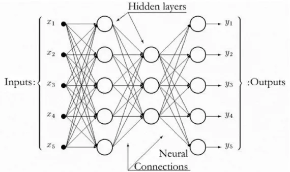
Fig. 4 - Structure of a feed-forward ANN with two hidden layers1_.

The purpose of these networks is to approximate some function 𝑓 by mapping an input domain to an output domain, which can be applied to solving complex problems such as prediction or classification from high dimensional data to a set of labels.

These networks consist of multiple layers, where the first layer is the input layer and the last is the output layer. The intermediate layers in the network are called the hidden layers and their number can vary. The use of multiple layers is what originated the term “Deep Learning”, with each additional layer creating an additional level of abstraction or representation.

Each layer is comprised of a number of neurons that represent activation values and it determines the width of that layer. Each neuron has a number of input weights that connect to each of the neurons of the previous layer, with the exception of the neurons in the input layer.

The activation values of the input layer are propagated forward in the direction of the output layer with no feedback connections where the outputs of the neurons are fed to previously activated neurons, hence the designation of “feedforward”.

(26)

The network is associated with a directed acyclic weighted graph describing how the functions are composed together. The network’s parameters consists of the weights and biases between layers.

The output activation values of a layer is represented as a vector, with each entry of the vector representing the activation value of a single neuron. The size of the vector corresponds to the number of neurons in that layer.

The weights between layers are represented as a 2D matrix, with each entry of the matrix at coordinates 𝑖, 𝑗 representing the weight connecting the neuron 𝑖 from layer 𝑙 − 1 to the neuron 𝑗 in the layer 𝑙.

The biases between layers is represented as a vector with the same size as the number of neurons in the next layer.

The mathematical notation of an FNN is defined as:

● 𝐿 , the number of layers in the network

● 𝑙 ∈ {1, . . . , 𝐿 − 1} , the index of the layer, starting at 1 as the first hidden layer and 𝐿 − 1 as the output layer

● 𝑁𝑙 _{, the number of neurons in layer 𝑙}

● 𝑛 ∈ {1, . . . , 𝑁𝑙_{− 1}} _{, the neuron index in layer 𝑙}

● ℎ𝑙 _{, the output vector of the activation values of the layer 𝑙}

● ℎ𝑛𝑙 , the activation value of the neuron 𝑛 in ℎ𝑙

● 𝑊𝑙 _{, the weight matrix of layer 𝑙}

● 𝑊_𝑖,𝑗𝑙 _{, the weight connecting the neuron 𝑖 from layer 𝑙 − 1 to the neuron 𝑗 in the layer 𝑙}

● 𝑏𝑙 _{, the bias vector of layer 𝑙}

● 𝑔𝑙_{(. ) , non linear activation function of layer 𝑙, it is assumed that the activation function}

of the input layer is a linear function. The activation function of the output layer is usually a different one from the hidden layers.

● 𝑦 , the output vector of the network ● 𝑦𝑛 , the output neuron 𝑛 of the network

(27)

The mathematical equation for the calculation of the output of each layer of the feedforward model is defined as:

● ℎ𝑙_{= 𝑔}𝑙_(𝑊𝑙_ℎ𝑙−1_{+ 𝑏}𝑙_{) , the activation values of a layer. With 𝑊}𝑙_ℎ𝑙−1_{being the dot product}

operation between the weight matrix of the current layer and the output values of the previous layer.

● 𝑦 = ℎ𝐿−1 _{, the activation values of the final output layer of the network}

3.1.2. Convolutional Neural Networks

Convolutional neural networks (CNNs) [54] are very similar to feedforward neural networks, in the sense that they still use the concept of neurons and that each neuron receives an input and performs an operation. The main distinction between the two architectures is that CNNs are a specialized kind of network for processing data that has a grid-like topology, such as time series and images.

A CNN is comprised of three types of layers: convolutional layers, pooling layers and fully connected layers.

(28)

Unlike a FNN, a CNN uses parameter sharing to decrease the number of parameters needed for high-dimensional input grids. A CNN always has the same number of parameters, even with bigger or smaller sized input grids. The parameters that a CNN uses are called kernels and they can be thought of as detectors for local patterns in data.

In a convolutional layer, the kernels are a set of small matrices or tensors that are applied to the input grid, by sliding the kernel across the grid with a defined stride length. Like in a neuron, the input values in each window are convolved with the weights of the same kernel, summed with a bias and then fed into a nonlinear function, giving a single output value for each input window. The result of applying one kernel to the input grid is another grid which is now designated as a channel or feature map. By applying multiple kernels to the same grid we get the same number of feature maps as the number of kernels in the convolutional layer. The resulting output grid now has a new depth of n feature maps and the remaining spatial dimension size depend on the previously defined window size, stride and input spatial dimension size.

The pooling layer is used to downsample along the spatial dimension of the input grid. A pooling layer, like a convolutional layer, defines a window size and a stride, on which a pooling operation is performed on the window’s input values. The most common pooling types are the max pooling and average pooling operations where the max or the average value of the window is returned. The result of a pooling operation is one value per window and it is combined with the other resulting values to create another smaller grid.

There is another type of pooling operation such as global pooling. Instead of applying a pooling operation on a window, global pooling applies the operation to each feature map individually without using a window, i.e. a global pooling operation transforms an input grid with a depth of n feature maps to a vector of size n. These pooling operations can be useful for transforming a dynamic sized input into a fixed sized output, like time series data.

When global pooling is not used and the input grid size is constant, the output grid of the convolution and pooling layers are flattened into a vector, which is then fed into a fully connected layer.

(29)

The fully connected layer serves to close the gap between feature detection and classification or prediction by using the flattened feature vector as input. A fully connected layer uses the exact same architecture as a FNN.

The mathematical notation for convolutional neural networks, while also referencing some of the previously defined notations for feedforward neural networks is defined as:

● 𝐾𝑙 _{, number of kernels in convolutional layer 𝑙 or the number of output feature maps}

● 𝑘 ∈ {1, . . . , 𝐾𝑙_{}, the index of feature map in layer 𝑙}

● 𝑏_𝑘𝑙 _{, bias parameter for kernel 𝑘 in convolutional layer 𝑙}

● 𝑋_𝑖,𝑗𝑙 _{, window of the input grid of convolutional layer 𝑙 at position 𝑖, 𝑗}

● 𝑊𝑘,𝑙 _{, weight matrix of kernel 𝑘 in convolutional layer 𝑙}

The equation to obtain a feature map 𝑘 in layer 𝑙 is defined as: ● ℎ_𝑖,𝑗𝑘,𝑙_{= 𝑔}𝑙_(𝑊𝑘,𝑙_{∗ 𝑋}

𝑖,𝑗𝑙 + 𝑏𝑘𝑙) , where 𝑊𝑘,𝑙 ∗ 𝑋𝑖,𝑗𝑙 denotes the convolution operation

between the kernel and input window, which have the same number of dimensions and size.

3.1.3. Gradient Descent

Gradient descent is a first order optimization algorithm [56][57] that utilizes the partial derivatives of the parameters to effectively decrease the value of a function.

To apply gradient descent to a neural network, the output must be a scalar value, which is often not the purpose of using neural networks. To circumvent this problem, a neural network is assigned a loss function that outputs a scalar value relating to the total classification or prediction loss of the network.

The main condition to make this method work is that both the functions used in the network and the loss function must be differentiable.

Most results inside a neural network can be expressed as a product of applying functions to the results of other functions:

(30)

● 𝐹(𝑥) = 𝑓(𝑔(𝑥))

To calculate the partial derivatives of a neural network, the chain rule is applied: ● 𝐹′(𝑥) = 𝑓′(𝑔(𝑥))𝑔′(𝑥)

And in the case of a neural network, we seek to calculate:

● 𝛿

𝐸

𝛿𝑤

_𝑖,𝑗 , the partial derivative of each weight with respect to the loss

The implementation of this optimization method for neural networks is called backpropagation [58], which propagates the derivatives backwards starting from the output loss in the direction of the input layer using the chain rule, thereby making the calculation of the partial derivatives computationally efficient. The gradients are multiplied by a constant scalar called the learning rate and it can be thought of as the step size of the model. A smaller learning rate leads to a slow but accurate traversal of the loss landscape, while a larger learning rate can lead to faster but inaccurate traversal of the loss landscape.

Using a stochastic gradient descent method, the dataset is split into mini-batches. These batches are used to calculate an estimate of the true loss of the neural network model, which then give an approximate gradient. This method leads to faster convergence and robustness with less computational efforts.

3.1.4. Loss Functions

There are several types of loss functions [56] which correspond to different purposes of machine learning such as regression, semantic segmentation and classification. The one we will present is a loss function used for the classification of data samples.

Categorical cross entropy

The categorical cross entropy loss is used for single label classification, meaning that each data sample belongs to only one class. It compares the predicted class distribution with the true class distribution, where the true class is represented as a one-hot encoded vector.

(31)

The categorical cross entropy loss is defined as:

● − ∑ (𝑡𝐶𝑖 𝑖 𝑙𝑜𝑔(𝑝𝑖)) , where 𝐶 is the number of classes, 𝑡𝑖 is the true probability of class

𝑖 and 𝑝𝑖 is the predicted probability of class 𝑖.

Since only one class is set to the value of 1 and the remaining values in 𝑡 are 0, it is equivalent to:

● −𝑙𝑜𝑔(𝑝𝑐) , where 𝑐 is the class index where 𝑡𝑐= 1.

Fig. 6 - Plot of the log loss of the categorical cross entropy loss function.

And this loss function can be viewed in figure 6, which can be interpreted as the heavy penalization of confident predictions that are wrong, i.e. predictions that approach the value of 0, although the true value is 1.

3.1.5. Activation Functions

Activation functions [56] are one of the essential components in deep learning that allow the generalization of neural networks in solving various tasks. Activation functions are required to be nonlinear so that neural networks can solve nonlinear problems, as is the case of the majority of real world problems. The careful design and choice of activation functions can improve training speed and convergence. Some of these are also loosely inspired by neuroscientific observations about how biological neurons compute.

(32)

Rectified Linear Unit

The rectified linear unit (ReLU) [59] activation function is the most popular in the deep learning community [60]. It has allowed deeper models to converge faster during training and achieve state of the art results.

It is defined as:

● 𝑓(𝑥) = 𝑚𝑎𝑥(0, 𝑥)

It is faster to compute than previously used activation functions, allows simpler initialization of network parameters, it induces sparse activation of the network’s hidden units, which is only about 50% that are activated with a non-zero output and it has less vanishing gradient problems when compared to the logistic sigmoid and hyperbolic tangent activation functions.

It is not without issues though. It is non-differentiable at zero, due to it being a piecewise function, but can be arbitrarily chosen to be either a 0 or 1. Some hidden units can become stuck in inactive states regardless of the input, which means that the gradient of the unit will always be 0 and the unit will stop training entirely. This will eventually decrease the model’s capacity to learn if the hyperparameters are not chosen carefully.

Leaky ReLU

The Leaky ReLU (LReLU) activation function [61] can be seen as an answer to the problem of inactive neurons which are a result of using the ReLU activation function.

It is defined as:

● 𝑓(𝑥) = 𝑥 , if 𝑥 > 0 ● 𝑓(𝑥) = 𝛼𝑥 , otherwise

The 𝛼 value is a static value that is defined during the creation of the neural network. It represents the slope of the negative section of the function and it allows the gradient to be different from 0, if 𝛼 ≠ 0, allowing the gradient to propagate through the neuron and to train the weights.

(33)

Softmax

The softmax function [56] converts a vector of arbitrary real values into another vector of the same shape such that the values are positive real numbers and their combined sum is equal to 1. This is useful for converting the raw non normalized outputs of a neural network into the probability of the input belonging to each one of the classes.

It is defined as: ● 𝑓(𝑦𝑖) =

𝑒𝑦𝑖 ∑𝑗_𝑗=1𝑒𝑦𝑗

Where 𝑦𝑖 is the raw output value of the neural network at index 𝑖 and 𝑓(𝑦𝑖) is the probability of

the data sample belonging to class 𝑖.

3.1.6. Regularization

Regularization is an important process in machine learning for the improvement of the generalization power of a model [56]. Dropout is a popular example of a regularization method for neural networks. Other regularization methods include the constraining of weights values of a neural network to be within a certain range.

Unit Norm Constraint

The unit norm constraint is a rule imposed on the model’s parameters such that their norm must be equal to 1. During training, the model updates its weights normally through gradient descent methods. After that, the weights are then normalized accordingly to have a vector norm of 1. This method can be effective as it allows the network to focus on training in terms of weight direction instead of scale, therefore increasing convergence speed and generalization. The unit norm constraint can also be specified to be for each individual neuron or for the entire weight matrix of the neural network’s layer.

(34)

3.2. State of the art pulmonary auscultation signal processing

3.2.1. Fourier Transform

The Fourier transform [62] is an integral transformation of a signal from the time domain to the frequency domain, allowing us to examine the signal in terms of the presence and strength of the various frequencies. The frequency domain has many advantages compared to the time domain of a signal. It is used to implement the most important methods of signal processing such as filtering, modulation and sampling of a signal. Therefore, it is the basis for most signal processing techniques and learning it is an important step towards understanding signal processing in general.

The calculation of the Fourier transform of a finite sequence of values is done with the Discrete Fourier Transform (DFT) method. The Fast Fourier Transform (FFT) is an efficient algorithm to calculate the DFT of a signal [62]. A spectrogram is the result of applying the DFT to multiple equally spaced overlapping small windows of the signal and stacking each window’s spectral result to create a new time-frequency representation, that shows the evolution of the signal’s frequency spectrum over time.

3.2.2. Power Spectral Density

The Power Spectral Density (PSD) [63] represents which frequency variations are strong and which are weak. The unit of the PSD is energy per frequency. PSD is an analysis method used when a measured signal in the time domain is transformed into the frequency domain through a Fourier transform. It is a useful tool to detect the frequencies and amplitudes of oscillatory signals and any periodicities in data.

3.2.3. Mel Spectrogram

A Mel Spectrogram (MS) represents an acoustic time-frequency representation of a sound. It is the result of transforming a spectrogram’s values into the mel scale [64]. The mel scale is a perceptual scale of pitches judged by humans to be equal in distance from one another. It is a way to mimic how the human ear responds to varying frequencies.

(35)

The mel frequency scale is defined as:

● 𝑚𝑒𝑙 = 2595 ∗ 𝑙𝑜𝑔 10(1 + ℎ𝑒𝑟𝑡𝑧/700)

and its inverse is:

● ℎ𝑒𝑟𝑡𝑧 = 700 ∗ (10 𝑚𝑒𝑙/2595_{− 1)}

The general method to obtain the mel spectrogram is through the following steps:

1. Separate signal to windows: Sample the input with windows of size n_fft, making hops of size hop_length each time to sample the next window.

2. Compute FFT for each window to transform from time domain to frequency domain. 3. Generate a mel scale: Take the entire frequency spectrum, and separate it into n_mels

evenly spaced frequencies according to the mel distance.

4. Generate Spectrogram: For each window, decompose the magnitude of the signal into its components, corresponding to the frequencies in the mel scale.

3.2.4. Mel-frequency Cepstral Coefficients

Mel-frequency cepstral coefficients (MFCCs) [65] are coefficients that collectively make up an mel-frequency cepstrum (MFC). MFCCs also take into account human perception for sensitivity at appropriate frequencies by converting the conventional frequency to mel scale. It is the most widely adopted and tested method for audio signal processing and speech recognition.

To calculate the MFCCs of a signal:

1. Separate signal to windows 2. Compute FFT for each window

3. Map the powers of the spectrum onto the mel scale

4. Compute the logs of the powers at each of the mel frequencies 5. Compute the Discrete Cosine Transform (DCT) of the mel log powers 6. Keep N amount of MFCCs

(36)

3.3. Discussion

We will not be utilizing the Dropout technique, since CNNs already have a form of parameter regularization because of its shared parameters.

(37)

Chapter 4: Materials and Methods

In this chapter, we describe the dataset that was used in this work to develop the classification methods, we describe the signal processing methodology, the libraries and tools used to implement the methods and the experimental methodology for comparing results of different methods. We also describe the implementation challenges, the proposed solutions, the advantages and limitations, our choices and our reasoning.

4.1. Dataset

Introduction

The International Conference on Biomedical and Health Informatics (ICBHI) 2017 respiratory sound database [66] was part of an organized scientific challenge to test and compare the robustness of state of the art techniques for lung sound processing and classification.

The creation of this dataset was motivated by the lack of large publicly available datasets that could be used to develop and compare different lung sound processing methods. Additionally, most of the sounds of small private datasets are clear and do not include environmental noise, which is unrealistic in clinical practice.

The dataset consists of a set of respiratory sound recordings and their respective annotation files. The audio samples were collected independently by two research teams: “Respiratory Research and Rehabilitation Laboratory of the School of Health Sciences, University of Aveiro” (Lab3R) and “Aristotle University of Thessaloniki” (AUTH) in two different countries, over several years. The dataset contains 920 annotated audio recordings which were collected from 126 participants.

Data collection

Each audio recording was obtained using multi-channel or single-channel acquisition method, with each channel representing an auscultation point of the participant and each channel is stored in a separate file. The auscultation points are: Anterior left (Al), Anterior right (Ar), Lateral left (Ll), Lateral right (Lr), Posterior left (Pl), Posterior right (Pr) and Trachea (Tc).

(38)

The types of equipment used by Lab3R to collect the lung sounds were:

● “Welch Allyn Meditron Master Elite Plus Stethoscope Model 5079-400” digital stethoscope ● Seven “3M Littmann Classic II SE” stethoscopes with a microphone in the main tube ● Seven air coupled electret microphones (C 417 PP, AKG Acoustics) located in capsules

made of teflon.

And the types of equipment used by AUTH were:

● “WelchAllyn Meditron Master Elite Plus Stethoscope Model 5079-400” digital stethoscope ● “3M Littmann 3200” digital stethoscope.

For the sake of simplicity, we will refer to these types of equipment with the following abbreviations:

● AKGC417L for “air coupled electret microphones” ● Litt3200 for “3M Littmann 3200”

● LittC2SE for “3M Littmann Classic II SE”

● Meditron for “Welch Allyn Meditron Master Elite Plus Stethoscope Model 5079-400”

Due to different equipment types used for the capture of the lung sounds, the sampling rate of each audio recording differs based on which was used.

Annotation

Each audio recording was annotated manually into individual respiratory cycles, where each cycle is given a starting timestamp, an ending timestamp, a binary number to indicate if the cycle contains a crackle and a binary number to indicate if the cycle contains a wheeze. The annotation process was done by respiratory health professionals.

In the case of the sound files originating from the Lab3R database, they were annotated by only one expert. And in the case of the AUTH database, they were annotated by three experienced physicians, two specialized pulmonologists, and one cardiologist.

(39)

Challenge

The official scientific challenge that was created for this dataset in the ICBHI 2017 is the classification of each individual respiratory cycle into one of four classes: Normal, Crackle, Wheeze, Both.

The dataset was split into training (60%) and testing (40%) sets, 2063 respiratory cycles from 539 recordings derived from 79 participants were included in the training set, while 1579 respiration cycles from 381 recordings derived from 49 patients were included in the testing set.

The challenge defines a set of metrics to evaluate the classification methods: Specificity (SP), Sensitivity (SE), Average score (AS) and Harmonic score (HS). These metrics are calculated as:

● SE = (Cc + Ww + Bb)/(C + W + B) ● SP = Nn/N

● AS = (SE + SP)/2

● HS = (2 ∗ SE ∗ SP)/(SE + SP)

Where N is the total number of normal sounds, Nn is the number of correctly classified normal sounds, C is the total number of crackle sounds, Cc is the number of correctly classified crackle sounds, W is the total number of wheeze sounds, Ww is the number of correctly classified wheezes, B is the total number of sounds that contain both crackle and wheeze sounds and Bb is the number of correctly classified sounds that contain both adventitious sounds.

SP can be interpreted as the method’s capability to correctly identify normal healthy sounds and SE is the method’s capability to correctly identify abnormal sounds.

Five international research teams submitted 18 systems in the first phase, then three of those teams uploaded 11 entries, then in the final phase of the challenge the two best teams presented their algorithms at ICBHI 2017.

(40)

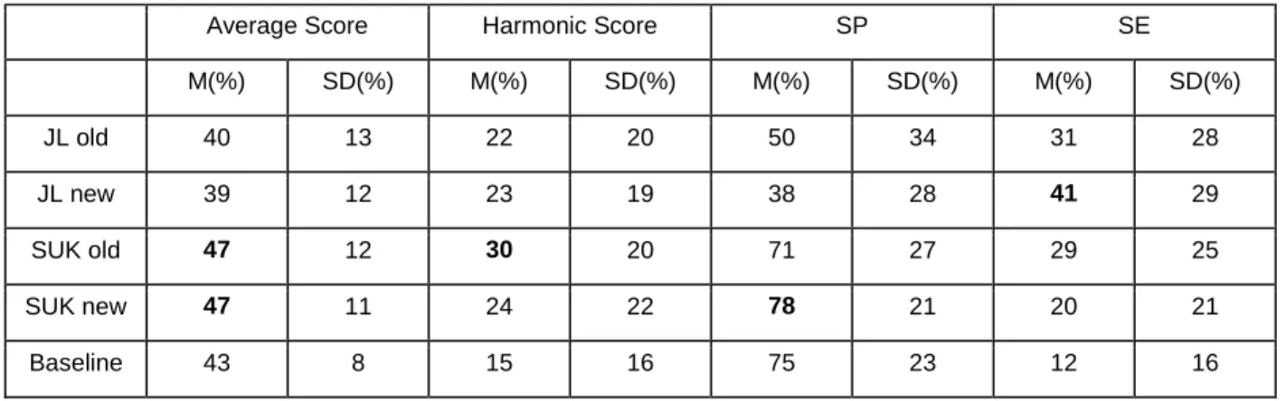
Table 1 - Test metrics for each method in the challenge. The best results for each of the metrics are highlighted in bold. With the mean and standard deviation for each metric.

Average Score Harmonic Score SP SE

M(%) SD(%) M(%) SD(%) M(%) SD(%) M(%) SD(%) JL old 40 13 22 20 50 34 31 28 JL new 39 12 23 19 38 28 41 29 SUK old 47 12 30 20 71 27 29 25 SUK new 47 11 24 22 78 21 20 21 Baseline 43 8 15 16 75 23 12 16

For more detailed information on the challenge dataset, like participant demographics or data distributions, please refer to the source paper [66].

New papers

Since the public release of the challenge dataset, there have been five studies [6-10], that we are aware of, that utilize this dataset.

So far, the best results that were obtained were from [6], by achieving SE = 0.56, SP = 0.736 and AS = 0.648 with a Noise Masking Recurrent Neural Network (NMRNN).

(41)

Dataset statistics

We did some preliminary statistics on the dataset before we started with the implementation of the methods, to get a better perspective and perform some early observations.

Table 2 - Statistics for each of the cycle classes.

Cycle Classes Cycle Count Patient Count Maximum Dur. (s) Minimum Dur. (s) Average Dur. (s)

Normal 3,642 124 16.163 0.2 2.6

Crackle 1,864 74 8.736 0.367 2.785

Wheeze 886 63 9.217 0.228 2.703

Crackle and Wheeze 506 35 8.592 0.571 3.06

Table 3 - Duration statistics for all recordings and cycles.

Duration Stats Recordings (s) Cycles (s) Maximum Duration 86.2 16.163 Minimum Duration 7.9 0.2

Mean Duration 21.5 2.7

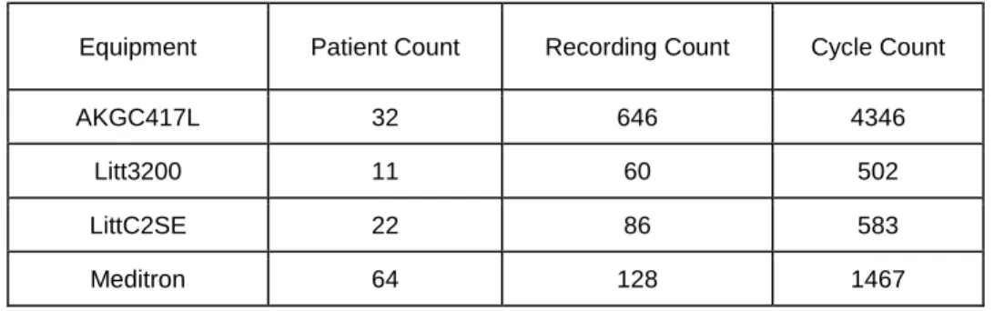
Table 4 - The patient sample count, the recording sample count and the cycle sample count for each of the equipment types.

Equipment Patient Count Recording Count Cycle Count

AKGC417L 32 646 4346

Litt3200 11 60 502

LittC2SE 22 86 583

(42)

Table 5 - The patient sample count, recording sample count and cycle sample count for each of the auscultation points.

Location Patient Count Recording Count Cycle Count

Al 80 162 1237 Ar 74 168 1277 Ll 42 77 604 Lr 54 112 819 Pl 61 139 1039 Pr 59 132 1003 Tc 53 130 919

Table 6 - The patient sample count, recording sample count and cycle sample count for each acquisition method.

Acquisition Mode Patient Count Recording Count Cycle Count

Multi-Channel 53 732 4929

Single-Channel 73 188 1969

Table 7 - Which equipment produces each of the sampling rates, as well as the patient sample count, recording sample count and cycle sample count for each of the sampling frequencies.

Sampling Rates Equipment Patient Count Recording Count

Cycle Count 44,100 Hz AKGC417L, LittC2SE, Meditron 109 824 5,821

4,000 Hz Litt3200, Meditron 16 90 1,016

(43)

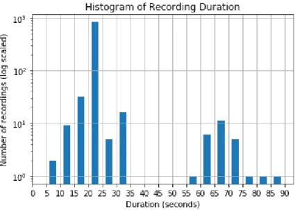
Fig. 7 - Recording duration distribution histogram with a log scaled y axis.

(44)

Discussion

Overall the dataset is unbalanced. The number of class samples in this dataset is very unbalanced, the duration of each recording session and individual respiratory cycle has a high variability, some participants lack a recording sample for at least one of their auscultation points or they have too many samples for some auscultation points.

Some recordings have extremely large respiratory cycles, which is actually due to an area of contact placement noise. The smaller duration respiratory cycles are most commonly the ending or starting cycles of a recording, which are most likely cut off.

And finally, the different sampling rates of the recordings, the equipment properties, noise artifacts and patient demographics also make it difficult to apply a simple method for classification.

4.2. Libraries

The project was implemented using the Python programming language [67] and Google

Colaboratory’s notebook environment [68]. The module that was used to load and downsample

the audio files was the Librosa module [69]. The Scipy module [70] was used to filter the audio files with a butterworth bandpass filter. The Tensorflow [71] library was used as the calculation method for MFCCs of an audio signal, while the kapre module [72] was used to calculate the PSD and MS of the signal. Finally, the Keras library [73] was used to implement the various neural network models, train the models and test them.

4.3. Signal processing methodology

To solve the problem of having different sampling rates, the audio recordings were downsampled to 4000 Hz, therefore the frequency range of the signal goes from 0 to 2000 Hz. The fundamental frequency range needed to detect crackles and wheezes is still within 0 to 2000 Hz.

To remove signal noise artifacts, we applied a 12th order butterworth bandpass filter [74] with cutoff frequencies of 120 Hz to 1800 Hz. This filter and cutoff frequencies were chosen from the method that obtained the best results in the official ICBHI 2017 challenge dataset paper [66].

(45)

Because of the varying amplitudes of the signals, which is caused by the different auscultation points and participant demographics, we chose to normalize the signal with respect to the mean and standard deviation of the signal. We normalized the respiratory cycles individually, so that other cycles with differing durations could not influence the resulting distribution.

We then calculate the PSD, MS and MFCCs of the signal at runtime, during cycle classification. The PSD and MS of the signal are converted to the decibel scale from 0 to -80, then the values are normalized to be within the range from 0 to 1 by adding 80 and then dividing by 80. The MFCCs are normalized with respect to the mean standard deviation of the coefficient values of the whole respiratory cycle signal.

4.4. Experimental methodology

In this section we present and discuss the methods used to solve various challenges that occurred during the project as well as the reasoning behind the choices that were made. We also present the methods for model evaluation and hyperparameter search.

Batch size issues

A critical aspect of Keras [73] is that, during the training process, the mini-batch used to train the model must be a static tensor, in other words, it cannot be a list of input tensors with differing sizes. Since a respiratory cycle can vary in duration length, in order to fit multiple audio signals in the same mini-batch, some form of padding or masking would be necessary. Other similar machine learning libraries have the same problem.

Masking a convolutional operation is a complex process and is time consuming. Padding the signals to fit the same size is easier to implement, although there was some concern that the model might learn to memorize the amount of padding in the signal or the border region between the actual signal and the padding values, resulting in overfitting and decreasing generalization capabilities.

A more reasonable way to get around these issues would be to calculate the gradients of the model for each input signal individually then averaging the gradients, which would be equivalent to the mini-batch gradient descent method. Unfortunately, the Keras library does not currently

(46)

allow for this type of method of mini-batch gradient calculation. This would then lead us to the manual implementation of such a method, but it would require us an extensive amount of time to accomplish, since there are many more underlying functions that happen during training.

In light of this, we decided to keep it much simpler by just using a mini-batch size of 1. There are other issues that arise from training a model using one sample at a time, such as training and optimizer stability. But we have found that utilizing the stochastic gradient descent optimization method [56] works better than other optimizers and can lead to less overfitting by using learning rate annealing.

This phenomenon can be explained roughly in the following way:

● Sharp local minima in the loss landscape are associated with poorer generalization and they produce larger gradients;

● By applying quick gradient updates to the model, it can end up on local sharp minima which would, in a way, propel the model to escape the region. By repeatedly applying this, the model will eventually reach a region that has flatter local minima that correlate with better generalization properties;

● By decreasing the learning rate gradually, the model becomes less sensitive to local minima, allowing it to decrease model loss;

Class imbalance

Due to the class imbalance in the dataset, all methods are trained with class undersampling. Undersampling is a technique with the purpose of balancing the number of samples per class during the training of machine learning models. It gives a more balanced estimate on the loss and statistics during model training, preventing the model from memorizing the minority classes first, which would technically increase the total accuracy, but the resulting model would be useless in practice.

The way this was implemented in this work is as follows: ● Repeat for N number of training epochs:

○ Sample random X amount of samples from each class ○ Shuffle samples

(47)

The maximum amount of samples to sample from each class is defined as the number of samples in the minority class. Undersampling is applied to both train and test sets during model training.

Dataset train/test split

During the splitting of the dataset into training and testing sets, we had the consideration of including all sounds belonging to a single patient in the same set to get a more accurate estimation of the model’s predictive power.

The methods were compared using the train/test split defined by the challenge [66]. Some of the audio samples that belong to the same patient are in different sets, therefore they were moved to the test set.

Lastly, the dataset was split into five folds to perform five-fold cross validation [75] and test the robustness of methods. The split was done in a random process so that the number of ‘Both’ class samples of each fold would be approximately the same.

Table 8 - Data distribution of the five folds.

Folds Normal Crackles Wheezes Both Total

1 1,168 415 265 100 1,948

2 847 521 217 107 1,692

3 590 280 150 99 1,119

4 533 476 143 101 1,253

5 504 172 111 99 886

(48)

Method evaluation and comparison

To evaluate and compare different methods, we use the metrics defined by the challenge [66], classification accuracy and the classification confusion matrix to assess and troubleshoot potential pitfalls in the training process. We evaluate and compare the final methods utilizing the five-fold cross validation method [75].

Model hyperparameter search method

The hyperparameter search process can be the most time consuming task relating to machine learning algorithms. To search for the best value combinations of the hyperparameters, we would have to perform an extensive search of all possible combinations. However, we have decided to experiment with only the most promising combinations based on facts and simple observations. We perform the hyperparameter search using the challenge train/test split. We don’t apply five-fold cross validation during the hyperparameter search due to the five five-fold increase in computation time of model training.

We test different signal features as input for the networks: ● Raw filtered audio signal (1D)

● PSD of the signal (2D) ● MS of the signal (2D) ● MFCCs of the signal (2D)

The hyperparameters for the networks and signal features are as follows:

● PSD parameters: PSD_N_DFT (DFT window size), PSD_N_HOP (DFT window stride), PSD_FMIN and PSD_FMAX (Resulting spectrum’s Y axis cutoff range, where only the frequencies inside FMIN to FMAX range are kept);

● MS parameters: MS_N_DFT (DFT window size), MS_N_HOP (DFT window stride), MS_FMIN, MS_FMAX (Resulting spectrum’s Y axis cutoff range, where only the frequencies inside FMIN to FMAX range are kept) and MS_N_MELS (How many mel conversion kernels to generate to then convert the spectrum to the mel scale);

● MFCC parameters: MFCC_N_DFT (DFT window size), MFCC_N_HOP (DFT window stride), MFCC_FMIN, MFCC_FMAX (Resulting spectrum’s Y axis cutoff range, where only the frequencies inside FMIN to FMAX range are kept), MFCC_N_MELS (How many mel