Introduction to Quantum Monte Carlo Simulations
for Fermionic Systems
Raimundo R. dos Santos
[email protected]Instituto de F´ısica, Universidade Federal do Rio de Janeiro,
Caixa Postal 68528, 21945-970, Rio de Janeiro, RJ, Brazil
Received on 27 August, 2002
We tutorially review the determinantal Quantum Monte Carlo method for fermionic systems, using the Hubbard model as a case study. Starting with the basic ingredients of Monte Carlo simulations for classical systems, we introduce aspects such as importance sampling, sources of errors, and finite-size scaling analyses. We then set up the preliminary steps to prepare for the simulations, showing that they are actually carried out by sampling discrete Hubbard-Stratonovich auxiliary fields. In this process the Green’s function emerges as a fundamental tool, since it is used in the updating process, and, at the same time, it is directly related to the quantities probing magnetic, charge, metallic, and superconducting behaviours. We also discuss the as yet unresolved ‘minus-sign problem’, and two ways to stabilize the algorithm at low temperatures.
1
Introduction
In dealing with systems of many interacting fermions, one is generally interested in their collective properties, which are suitably described within the framework of Statistical Mechanics. Unlike insulating magnets, in which the spin degrees of freedom are singled out, the interplay between charge and spin is responsible for a wealth of interesting phenomena (orbital degrees of freedom may also be in-cluded, but they add enormously to complexity, and shall not be considered here). Typical questions one asks about a system are related to its magnetic state (Is it magnetic? If so, what is the arrangement?), to its charge distribution, and to whether it is insulating, metallic, or superconductor.
A deeper understanding of the interplay between spin and charge degrees of freedom can be achieved through models, which, while capturing the basic physical mech-anisms responsible for the observed behaviour, should be simple enough to allow calculations of quantities compara-ble with experiments. The simplest model describing in-teracting fermions on a lattice is the single band Hubbard model [1], defined by the grand-canonical Hamiltonian
H= t
X
hi;ji;
y i
j
+H::
+U X
i n
i" n
i#
X
i
n i"
+n i#
; (1)
wheretis the hopping integral (which sets the energy scale, so we take t = 1 throughout this paper), U is the on-site Coulomb repulsion, is the chemical potential con-trolling the fermion density, andi runs over the sites of a
d-dimensional lattice; for the time being, we consider hop-ping between nearest neighbours only, as denoted byh:::i. The operators
y i
and i
respectively create and annihilate a fermion with spin on the (single) orbital centred at i, whilen
i
y i
i. The Hubbard model describes the com-petition between opposing tendencies of itinerancy (driven by the hopping term), and localization (driven by the on-site repulsion). For a half-filled band (one fermion per site), it can be shown [2] that in the limit of strong repulsion the Hubbard Hamiltonian reduces to that of an isotropic antifer-romagnetic Heisenberg model with an exchange coupling J =4t
2 =U.
If we let the couplingUassume negative values, one has theattractiveHubbard model. Physically, thislocal attrac-tion can have its origin in the coupling of fermions to ex-tended (through polaron formation) or local phonons (such as vibrational modes of chemical complexes) [3]. Given that its weak coupling limit describes the usual BCS the-ory, and that the real-space pairing is more amenable to nu-merical calculations, this model has also been useful in elu-cidating several properties of both conventional and high-temperature superconductors [3].
The Hubbard model [even in its simplest form, Eq. (1)] is only exactly soluble in one dimension, through the Bethe ansatz; correlation functions, however, are not directly avail-able. In higher dimensions one has to resort to approxi-mation schemes, and numerical techniques such as Quan-tum Monte Carlo (QMC) simulations have proven to be crucial in extracting information about strongly correlated fermions.
al-gorithms have been proposed. Their classification is var-ied, and depends on which aspect one wishes to single out. For instance, they can be classified according to whether the degrees of freedom lie in the continuum or on a lat-tice; or whether it is a ground-state or a finite-temperature framework; or whether it is variational or projective; or even according to some detailed aspect of their implementation, such as if an auxiliary field is introduced, or if a Green’s function is constructed by the power method. Excellent broad overviews of these algorithms are available in the lit-erature, such as Refs. [7,8], so here we concentrate on the actual details of the grand-canonical formulation with aux-iliary fields leading to fermionic determinants [9]. We will pay special attention to the implementations and improve-ments achieved over the years [10-14]. We will also have in mind primarily the Hubbard model, but will not discuss at length the results obtained; instead, illustrative references will be given to guide the reader to more detailed analyses, and we apologize for the omitions of many relevant papers, which was dictated by the need to keep the discussion fo-cused on this particular QMC implementation, and not on the Hubbard (or any other) model.
In line with the tutorial purpose of this review, we intro-duce in Sec. 2 the basic ingredients of Monte Carlo simula-tions, illustrated for ‘classical’ spins. In this way, we have the opportunity to draw the attention of the inexperienced reader to the importance of thorough data analyses, com-mon to both classical and quantum systems, before embark-ing into the more ellaborate quantum formalism. Prelimi-nary manipulations, approximations involved, and the nat-ural appearance of Green’s functions in the framework are then discussed in Sec. 3. In Sec. 4, we describe the updat-ing process, as well as the wide range of average quantities available to probe different physical properties of the sys-tems. We then address two of the main difficulties present in the simpler algorithm presented so far: the still unresolved ‘minus-sign problem’ (Sec. 5), and the instabilities at low-temperatures, (Sec. 6) for which two successful solutions are discussed. Conclusions and some perspectives are then presented in Sec. 7.
2
Monte Carlo simulations for
‘clas-sical’ spins
Our aim is to calculate quantities such as the partition func-tion (or the grand-partifunc-tion funcfunc-tion) and various averages, including correlation functions; these quantities are obtained by summing over all configurations of the system. For defi-niteness, let us consider the case of the Ising model,
H= J X
hi;ji
z i
z j
; (2)
whereJis the exchange coupling and z i
=1. For a lattice withN
s sites there are 2
N s
possible con-figurations in phase space. Clearly all these concon-figurations
are not equally important: recall that the probability of oc-currence of a given configuration,C, with energy E(C), is / exp[ E(C)=k
B
T℄. Therefore, from the numerical point of view, it is not efficient to waste time generatingall configurations. Accordingly, the basic Monte Carlo strat-egy consists of animportance sampling of configurations [5,6]. This, in turn, can be implemented with the aid of theMetropolis algorithm [4], which generates, in succes-sion, a chain of the most likely configurations (plus fluctua-tions; see below). Starting from a random spin configuration
C j
1 ;
2 ;:::;
Ns
i, one can imagine a walker visiting every lattice site and attempting to flip the spin on that site. To see how this is done, let us suppose the walker is cur-rently on sitei, and callC
0
the configuration obtained from Cby flipping
i. These configurations differ in energy by
E =E(C
0
) E(C) =2J i
P 0 j
j, where the prime in the sum restrictsjto nearest neighbour sites ofi. The ratio between the corresponding Boltzmann factors is then
r 0
p(C
0 )
p(C)
=exp( E=k B
T): (3)
Thus, ifE < 0,C 0
should be accepted as a new config-uration in the chain. On the other hand, ifE > 0the new configuration is less likely, but can still be accepted with probabilityr
0
; this possibility simulates the effect of fluctuations. Alternatively [6], one may adopt theheat-bath algorithm,in which the configurationC
0
is accepted with probability
r r
0
1+r 0
(4) In both cases, the local character of the updating of the con-figuration should be noted; that is, the acceptance of the flip does not influence the state of all other spins. As we will see, this is not true for quantum systems.
The walker then moves on, and attempts to flip the spin on the next site through one of the processes just described. After sweeping through the whole lattice, the walker goes back to the first site, and starts attempting to flip spins on all sites again. One should make sure that the walker sweeps through the lattice many times so that the system thermal-izes at the given temperature; thiswarming-upstage takes typically between a few hundred and a few thousand sweeps, but it can be very slow in some cases.
Once the system has warmed-up, we can start ‘measur-ing’ average values. Suppose that at the end of the -th sweep we have stored a valueA
for the quantity A. It would therefore seem natural that afterN
a such sweeps, an estimate for the thermodynamic averagehAishould be given by
A=
1
N a
Na X
=1 A
: (5)
However, theA
A 1
; A 2
;:::; A
G, leading to a final average
hAi= 1
G G X
g=1 A g
: (6)
Ideally, one should alternate N
n sweeps without taking measurements withN
a sweeps in which measurements are taken.
Once theA
g’s can be considered as independent random variables, the central limit theorem [15] applies, and the sta-tistical errorsin the average ofAare estimated as
ÆA=
hA 2
i hAi 2
G
1=2
: (7)
In addition,systematic errors must be taken into con-sideration, the most notable of which are finite-size effects. Indeed, one should have in mind that usually there are two important length scales in these calculations: the linear size, L, and the correlation length of the otherwise infinite
sys-tem, jT T
j
. A generic thermodynamic quantity, X
L
(T), then scales as [16] X
L
(T)=L x=
f(L=); (8)
wherexis a critical exponent to be defined below, andf(z) is a scaling function with very specific behaviours in the lim-itsz 1andz 1. In the former limit it should reflect the fact that the range of correlations is limited by the finite system size, and one must have
X L
(T)'onst:L x=
; forL; (9)
so that an explicitL-dependence appears. On the other hand, when correlations do not detect the finiteness of the system, the scaling function must restore the usual size-independent form,
X L
(T)'jT T
j x
; forL; (10) this defines the critical exponentx. This finite-size scaling (FSS) theory can be used in the analysis of data, thus setting the extrapolation towards the thermodynamic limit on firmer grounds.
As a final remark, we should mention for completeness that the actual implementation of the Monte Carlo method for classical spins can be optimized in several aspects, such as using bit-strings to represent states [17], and broad his-tograms to collect data [18].
3
Determinantal
Quantum
Monte
Carlo: Preliminaries
The above discussion on the Ising model was tremendously simplified due to the fact that the eigenstates of the Hamilto-nian are given as products over single particle states. Quan-tum effects manifest themselves in the fact that different terms in the Hamiltonian do not commute. In the case of
the Hubbard model, the interaction and hopping terms do not commute with each other, and, in addition, hopping terms involving the same site also do not commute with each other. Consequently, the particles lose their individ-uality since they are correlated in a fundamental way.
One way to overcome these non-commuting aspects [9] is to notice that the Hamiltonian contains terms which are bi-linear in fermion operators (namely, the hopping and chemi-cal potential terms) and a term with four operators (the inter-action term). Terms in the former category can be trivially diagonalized, but not those in the latter. Therefore, when calculating the grand partition function,
Z=Tre H
; (11)
where, as usual,Trstands for a sum over all numbers of par-ticles and over all site occupations, one must cast the quartic term into a bilinear form.
To this end, we first separate the exponentials with the aid of the Suzuki-Trotter decomposition scheme [19], which is based on the fact that
e
(A+B) =e
A e
B +O
()
2
[A;B℄; (12) for A and B generic non-commuting operators. Calling K andV, respectively the bilinear and quartic terms in the Hubbard Hamiltonian, we introduce a small parameter through =M, and apply the Suzuki-Trotter formula as
e
(K+V) = e
K+V
M
=
= e K
e V
M
+O
() 2
U
:(13) The analogy with the path integral formulation of Quantum Mechanics suggests that the above procedure amounts to theimaginary-timeinterval(0;)being discretized intoM slices separated by the interval.
In actual calculations at a fixed inverse temperature, we typically set =
p
0:125=Uand chooseM==. As evident from Eq. (13), the finiteness of is also a source ofsystematic errors;these errors can be downsized by obtaining estimates for successively smaller values of (thus increasing the number,M, of time slices) and extrap-olating the results to ! 0. Given that this complete procedure can be very time consuming, one should at least check that the results are not too sensitive to by per-forming calculations for two values of and comparing the outcomes.
Having separated the exponentials, we can now workout the quartic terms inV. We first recall a well known trick to change the exponential of the square of an operator into an exponential of the operator itself, known as the Hubbard-Stratonovich (HS) transformation,
e 1 2 A
2
p 2
Z 1
1 dxe
1 2 x
2 xA
; (14)
A; this result is immediately obtained by completing the squares in the integrand. However, before a transformation of this kind can be applied to the quartic term of the Hub-bard Hamiltonian, squares of operators must appear in the argument of the exponentials. Since for fermions one has n
2
n
= 0;1(here we omit lattice indices to simplify the notation), the following identities – in terms of the lo-cal magnetization,m n
" n
#, and of the local charge, nn
" +n
#– will suit our purposes:
n "
n #
= 1
2 m
2 +
1
2
n; (15a)
n "
n #
= 1
2 n
2 1
2
n; (15b)
n "
n #
= 1
4 n
2 1
4 m
2
; (15)
The following points are worth making about Eqs. (15), in relation to the HS transformation: (i) an auxiliary field will be introduced for each squared operator appearing on the RHS’s above; (ii) the auxiliary field will couple to the local magnetization and to the local charge when, respectively, Eqs. (15a) and (15b) are used; (iii) Eqs. (15a) and (15b) are respectively used for the repulsive and for the attractive models.
Instead of the continuous auxiliary field of Eq. (14), in simulations it is more convenient to work withdiscreteIsing variables, s = 1 [10]. Inspired by Eq. (14), using Eq. (15a), and taking into account thats
2
1, it is straightfor-ward to see that
e
Un
" n
# =
1
2 e
U 2
n X
s=1 e
sm =
= 1
2 X
s=1 Y
=";# e
(s+ U
2 )n
; U >0;
(16) where the grouping in the last equality factorizes the con-tributions from the two fermion spin channels, = +; (respectively corresponding to =";#), and
osh=e jUj=2
: (17)
In the attractive case, the coupling to the charge [Eq. (15b)] is used in order to avoid a complex HS transforma-tion; we then get
e jUjn
" n
# =
1
2 X
s=1 Y
=";# e
(s+ jUj
2 )(n
1 2 )
; U <0;
(18) withstill being given by Eq. (17).
The HS transformations then replace the on-site inter-action by a fluctuating fieldscoupled to the magnetization or to the charge, in the repulsive or attractive cases, respec-tively. As a consequence, the argument of the exponential depends explicitly onin the former case, but not in the lat-ter. As we will see below, this very important difference is responsible for the absence of the ‘minus-sign problem’ in the attractive case.
We now replace the on-site interaction on every site of the space-time lattice by Eqs. (16) or (18), leading to the sought form in which only bilinear terms appear in the ex-ponential. For the repulsive case we get
Z=
1
2
L d
M
Tr fsg
Tr 1 Y
`=M Y
=";# e
P
i;j
y i
Kij j
e
P i
y i
V i
(`) i
; (19)
d
where the traces are over Ising fields and over fermion oc-cupancies on every site, and the product from` = M to 1 simply reflects the fact that earlier ‘times’ appear to the right. The time-slice index`appears through the HS field s
i (`)in
V i
(`)= 1
s
i (`)+
U
2
; (20)
which are the elements of the N s
N
s diagonal matrix V
(`). One also needs theN s
N
shopping matrix K, with elements
K ij
= (
t ifiandjare nearest neighbours, 0 otherwise
(21)
For instance, in one-dimension, and with periodic boundary conditions, one has anLLmatrix,
K= 0
B B B B B
0 t 0 0 t
t 0 t 0 0
0 t 0 0 0
..
. ... ... ... ... ...
t 0 0 t 0
1
C C C C C A
: (22)
With bilinear forms in the exponential, the fermions can be traced out of Eq. (19) according to the development of Appendices A and B. From Eq. (124), with the spin in-dices reintroduced, and with the identificatione
h
e K
e V
(`)
, we have
Z=
1
2
L d
M
Tr
fsg Y
det
1+B
M
B M 1
:::B 1
; (23) where we have defined
B `
e K
e V
(`)
; (24)
in which the dependence with the auxiliary Ising spins has not been explicitly written, but should be understood, since they come in through the matrixV
(`). Introducing O
(fsg)1+B M
B M 1
:::B 1
; (25)
we arrive, finally, at
Z =
1
2
L d
M
Tr
fsg detO
"
(fsg)detO #
(fsg)=
=
Tr
fsg(fsg); (26)
where the last equality defines an effective ‘density matrix’, (fsg).
We have then expressed the grand partition function as a sum over Ising spins of a product of determinants. If the quantity under the Tr were positive definite, it could be used as a Boltzmann weight to perform importance sampling over the Ising configurations. However, the product of determi-nants can indeed be negative for some configurations, giving rise to the ‘minus-sign problem’; see Sec. 5.
In order to implement the above framework, the need for another approximation is evident from Eq. (24): one needs to evaluate the exponential of the hopping matrix, which, in the general case, is neither an analytically simple oper-ation, nor efficiently implemented numerically. By consid-ering again a one-dimensional system, we see that different powers ofK; as given by Eq. (22), generate many differ-ent matrices. However, we can introduce a ‘checkerboard break-up’ by writing
K=K (a) x
+K (b) x
; (27)
such thatK (a)
involves hoppings between sites 1 and 2, 3 and 4,:::, whileK
(b)
involves hoppings between sites 2 and 3, 4 and 5,:::. We now invoke the Suzuki-Trotter decompo-sition scheme to write
e K
=e K
(a) x
e K
(b) x
+O
() 2
; (28) which leads to systematic errors of the same order as before. With this choice of break-up, even powers ofK
() x
; =
a;b;become multiples of the identity matrix, and we end up with a simple expression,
e K
() x
=K () x
sinh( t)+1osh(t); (29) which is very convenient for numerical calculations. The breakup of Eq. (28) can be generalized to three dimensions as follows
e K
=e K
(a) z
e K
(a) y
e K
(a) x
e K
(b) z
e K
(b) y
e K
(b) x
+O
() 2
; (30)
d
where the separation along each cartesian direction is simi-lar to that for the one-dimensional case.
And, finally, we must discuss the calculation of average values. For two operatorsAandB, their equal-‘time’ cor-relation function is
hABi= 1
Z
Tr
fsg Tr
"
AB Y
` e
K e
V
(`) #
: (31) If we now define the fermion average – or Green’s function – for a given configuration of the HS fields as
hABi fsg
1
(fsg) Tr
"
AB Y
` e
K e
V
(`) #
;
(32) the correlation function becomes
hABi= 1
Z
Tr
fsg hABi
fsg
(fsg): (33)
At this point it should be stressed the important role played by the Green’s functions in the simulations. Firstly,
according to Eq. (33), the average value of an operator is straighforwardly obtained by sampling the corresponding Green’s function over the HS configurations weighted by (fsg). Secondly, as it will become apparent in Sec. 4, the single particle Green’s function,h
i
y j
i
fsg, plays a central role in the updating process itself. In Appendix C we obtain this quantity as the elementijof anN
s
N
smatrix [11,8]: h
i
y j
i fsg
= h
1+B M
B M 1
:::B 1
1 i
ij
; (34) which is, again, in a form suitable for numerical calcula-tions. And, thirdly, within the present approach the fermions only interact with the auxiliary fields, so that Wick’s the-orem [20] holds for a fixed HS configuration [11,8,14]; the two-particle Green’s functions are then readily given in terms of the single-particle ones as
h y i1
i2
y i3
i4
i fsg
=h y i1
i2
i fsg
h y i3
i4
i fsg
+
+h y i1
i4
i fsg
h i2
y i3
i fsg
where the indices include spin, but since the"and#spin channels are factorized [c.f. Eq. (32)], these fermion aver-ages are zero if the spins are different. All average values of interest are therefore calculated in terms of single-particle Green’s functions.
As will be seen, unequal-time correlation functions are also important. We define the operatorain the ‘Heisenberg picture’ as
a(`)a()=e H
ae H
; `; (36)
so that the initial time is set to = with this discretiza-tion, anda
y
(`)6=[a(`)℄ y
. In Appendix D, we show that the unequal-time Green’s function, for`
1 >`
2, is given by [11] G
ij
(` 1
;` 2
) h
i (`
1 )
y j
(` 2
)i fsg
=
=
B `1
B `1 1
:::B `2+1
g
(` 2
+1)
ij ; (37) in which the Green’s function matrix at the`-th time slice is defined as
g
(`)[1+A
(`)℄ 1
; (38)
with A
(`)B
` 1
B ` 2
:::B 1 B
M
:::B `
: (39)
The reader should notice the order in which the products ofB’s are taken in Eqs. (34), (37), and (39); in Eq. (37), in particular, the product runs from`
2
+1to`
1, and not cycli-cally as in Eq. (39). Also, for a given configurationfsgof the HS spins, the equal-time Green’s functions do display a time-slice dependence, as expressed by Eq. (38); they only become (approximately) equal after averaging over a large number of configurations.
For future purposes, we also define
~ g ij
[1 g ℄ ij
; and ~ G ij
[1 G℄ ij
: (40)
4
Determinantal
Quantum
Monte
Carlo: The Simulations
The simulations follow the lines of those for classical sys-tems, except for both the unusual Boltzmann weight, and the fact that one sweeps through a space-time lattice. With the parameters of the Hamiltonian,U and, as well as the temperature, fixed from the outset, we begin by generating, say a random configuration,fsg, for the HS fields. Since the walker starts on the first time-slice, we use the defini-tion, Eq. (34), to calculate the Green’s function at`=1. As the walker sweeps the spatial lattice, it attempts to flip the HS spin at every one of theN
spoints.
At this point, it is convenient to picture the walker at-tempting to flip the HS (Ising) spin on a generic site,iof a generic time slice,`. If the spin is flipped, the matricesB
" ` andB
#
` change due to the element
iiof the matricesV "
(`) andV
#
(`), respectively, being affected; see Eqs. (20) and (24). The expression for the change in the matrix element, ass
i
(`)! s i
(`), is
ÆV ij
(`)V ij
(`; s) V ij
(`;s)= 2s i
(`)Æ ij
; (41) which allows us to write the change inB
`
as a matrix prod-uct,
B `
![B ` ℄
0 =B
`
`
(i); (42)
where the elements of the matrix `
(i)are
[ `
(i)℄ jk
= 8 <
:
0 if j6=k ; 1 if j=k6=i; e
2si(`)
if j=k=i:
(43)
Let us now callfsg 0
andfsg, the HS configurations in which all Ising spins are the same, except for those on site (i;`), which are opposite. We can then write the ratio of ‘Boltzmann weights’ as
r 0
= (fsg
0 )
(fsg) =
detO "
(fsg 0
)detO #
(fsg 0
)
detO "
( fsg)detO #
(fsg) =R
" R
# ; (44) where we have defined the ratio of fermion determinants as
R
detO
(fsg
0 )
detO
(fsg)
: (45)
It is important to notice that one actually does not need to calculate determinants, sinceR
is given in terms of the Green’s function:
R
=
det[1+A
(`) `
(i)℄
det[1+A
(`)℄ =
=det
1+A
(`) `
(i)
g
(`)
=
=det
1+ 1 g
(`)
`
(i) 1
=
=1+ 1 g ii
(`)
e
2s i
(`) 1
: (46) The last equality follows from the fact that
`
(i) `
(i) 1 (47)
is a matrix such that all elements are zero, except for thei-th position in the diagonal, which is
`
(i) e 2s
i (`)
1. With this simple form forR
, the heat-bath algorithm is then easily implemented, with the probability of acceptance of the new configuration being given by Eq. (4), with Eqs. (44) and (46).
If the new configuration is accepted, thewholeGreen’s function for the current time slice must be updated, not just its elementii; this is the non-local aspect of QMC simula-tions we referred to earlier. There are two ways of updating the Green’s function. One can either compute the ‘new’ one from scratch,through Eq. (38), oriteratethe ‘old’ Green’s function, by following along the lines that led to Eq. (46), which yields
g
(`)=
1+ 1 g
(`)
(i)
1
g
An explicit form for g
(`)is obtained, e.g., by first using an ansatz to calculate the inverse of the matrix in square brack-ets above,
1+ 1 g
(`)
`
(i)
1
=1+x 1 g
(`)
`
(i) (49) wherexis to be determined from the condition that the prod-uct of both matrices in Eq. (49) is1. Using the fact that
`
(i) is very sparse, one arrives at
x= 1
R
; (50)
withR
being given by Eq. (46). The element
jk of the Green’s function is then updated according to
g jk
(`)=g jk
(`) h
Æ ji
g ji
(`) i
`
(i)g ik
(`)
1+[1 g ii
(`)℄ `
(i)
: (51) Alternatively, one could arrive at the same result by solving a Dyson’s equation forg
jk
(`)[8].
After the walker tries to flip the spin on the last site of the`-th time slice, it moves on to the first site of the (`+1 )-th time slice. We )-therefore need )-the Green’s function for the (`+1)-th time slice, which, as before, can be calculated either from scratch, or iteratively from the Green’s function for the`-th time slice. Indeed, by comparing[ g
(`+1)℄
1
with[g
(`)℄ 1
, as given by Eq. (38), it is easy to see that
g
(`+1)=B ` g
(`)
B
`
1
; (52)
which can be used to compute the Green’s function in the subsequent time slice.
While the computation from scratch of the new Green’s function takesN
3
s operations, the iterations [Eq. (51) and (52)] only take N
2
s operations. Hence, at first sight the latter form of updating should be used. However, rounding errors will be amplified after many iterations, thus deterio-rating the Green’s function calculated in this way; see Sec. 6. A solution of compromise is to iterate the Green’s func-tion while the walker sweeps all spatial sites of ~
` ( 10) time slices, and then to compute a new one from scratch when the (~
`+1)-th time slice is reached. This ‘refreshed’ Green’s function will then be used to start the iterations again. Clearly, one should checkgfor accuracy, by com-paring the updated and refreshed ones at the (~
`+1)-th time slice; if the accuracy is poor,~
`must be decreased.
For completeness, we now return to the situation de-scribed in the beginning of this Section, in which the walker attempts to flip the HS spins on every spatial site of the`=1 time slice. Whenever the flip is accepted, the Green’s func-tion is updated according to Eq. (51). After sweeping all spatial sites, and before the walker moves on to the first site of the ` = 2time slice, we use Eq. (52) to calculate g
(2). The walker then sweeps the spatial sites of this time-slice, attempting to flip every spin; if the flip is accepted, the Green’s function is updated according to Eq. (51). As men-tioned above, this procedure is repeated for the next ~
`time
slices. After sweeping the last one of these, a new Green’s function is calculated from the definition, Eq. (38). For the subsequent ~
` time slices the iterative computation of gis used, and so forth.
Similarly to the classical case, one sweeps the space-time lattice several space-times (warm-up sweeps) before calculat-ing average values. After warmcalculat-ing up, one starts the ‘mea-suring’ stage, in which another advantage of the present ap-proach manifests itself in the fact, already noted, that all av-erage quantities are expressed in terms of the Green’s func-tions. This brings us to the discussion of the main quantities used to probe the physical properties of the system, and how they relate to the Green’s functions.
We start with the calculation of the occupation,n. It is given by
n =
1
MN s
X
i;` X
h
y i
(`) i
(`)i=
= 1
MN s
X
i;` X
hh1 g ii
(`)ii; (53) where the first equality illustrates that the ensemble average (i.e.,over both fermionicandHS fields)hn
i" (`)+n
i# (`)iis itself averaged over allMN
ssites of the space-time lattice. In the second equality the fermion degrees of freedom have been integrated out (hence the Green’s functions), and the average over HS fields, represented by double brackets, is to be performed by importance sampling overN
aHS configu-rations [c.f.Eq. (33)]. We then have
hhg ij
(`)ii' 1
N a
Na X
=1 g
ij
(`): (54)
It should be reminded that since these are grand-canonical simulations, the chemical potential must be cho-sena prioriin order to yield the desired occupation. The chemical potential leading to half filling in the Hubbard model (with nearest-neighbour hopping only) is obtained by imposing particle-hole symmetry [2,21]: one getsn=1for =U=2for allT andN
s. Away from half-filling, one has to determineby trial and error, which must be done repeat-edly, since the dependence ofnwith(for givenN
sand U) itself varies with temperature. Overall, the dependence ofn withindicates that the Hubbard model is an insulator at half filling in any dimension: indeed, the compressibility
1
V
V
P
T; =
1
n 2
n
T
; (55)
whereV andP are the volume and pressure, respectively, vanishes at = U=2, so that no particles can be added to the system; see, e.g., Ref. [22] for explicit data forn()in two dimensions.
The magnetic properties are probed in several ways. Since the components of the magnetization operator are
m x i
y
+
y
m y i i y i" i# y i# i" ; (56b) m z i n i" n i# ; (56)
Wick’s theorem [Eq. (35)] allows one to obtain the equal-time spin-density correlation functions as
hm z i m z j
i=hhg~ " ii ~ g " jj
+~g " ij g " ij ~ g " ii ~ g # jj ~ g # ii ~ g " jj
+~g # ii ~ g # jj
+g~ # ij g # ij ii; (57a) hm x i m x j
i=hhg~ " ij g
# ij
+~g # ij g " ij ii; (57b)
and a similar expression for theyycorrelations. It is under-stood that theg’s are to be evaluated at the same time slice as them’s on the LHS.
If spin rotational symmetry is preserved, as in the case of a singlet ground state, Eqs. (57a) and (57b) should yield the same result. This is indeed the case for average values, but, in practice, transverse (i.e.,xxandyy) correlations are much less noisy than the longitudinal ones [23]; this can be traced back to the discrete HS transformation, which singles out thez component by coupling the auxiliary fields to the m
z
’s. It should also be pointed out that a possible ferromag-netic state (either saturated or just a non-singlet one) would break this symmetry.
Settingi=jin Eqs. (57) leads to the local moment,
hm 2 i
i=h( m x i
) 2
+( m y i )
2 +( m
z i )
2
i (58)
which measures the degree of itinerancy of the fermions. For instance, considering again the Hubbard model at half fill-ing,h( m
i )
2
i, =x;y;z;decreases from 1, in the frozen-charge state (i.e.,whenU !1), to 1/2, in the metallic state (U =0).
One can collect the contributions to the spin-spin corre-lation functions from different sites, and calculate the equal-time magnetic structure factor as
S(q)= 1 N s X ij e iq(i j) hS i S j i; (59) whereS i =m i
=2, since~=1.S(q)shows peaks at val-ues ofqcorresponding to the dominant magnetic arrange-ments. For the Hubbard model in one dimension, S(q) has peaks at q = 2k
F
= n, corresponding to quasi-long range order (i.e.,algebraic spatial decay of correlations) in the ground state; one refers to this as a state with a spin-density wave[24]. In two dimensions, and at half filling, the peak located at q = (;) [25] signals N´eel order in the ground state; away from half-filling, the system is a param-agnet [11,25] with strong AFM correlations at incommen-surateq’s [22].
The non-commutation aspects imply that the suscepti-bility is given by [20]
(q)= 1 N s X ij e iq(i j) Z 0 d hS i ()S
j
i: (60)
In the discrete-time formulation, the integral becomes a sum over different time intervals, which is carried out with the aid of the unequal-time Green’s functions. Focusing on one of the components of the scalar product above, sayz, we have hm i (` 1 )m j (` 2 )i = X ; 0 h ( 2Æ 0 1) ~ g ii (` 1 )~g 0 jj (` 2 ) + Æ 0 ~ G ij (` 1 ;` 2 )G ij (` 1 ;` 2 ) i : (61) Similarly to the magnetic properties, one can also in-vestigate whether or not there is the formation of a charge density wave [26,27]. Withn
i =n
i" +n
i#, theequal-time correlation function is given by
hn i n j i= X ; 0 h ~ g ii ~ g 0 jj +Æ 0 ~ g ji g ij i ; (62) in terms of which the charge structure factor becomes
C(q)= 1 N s X ij e iq(i j) hn i n j i: (63)
It is also useful to define a charge susceptibility as
N(q)= 1 N s X ij e iq(i j) Z 0 dhn i ()n j i; (64) where, in the discrete time formulation, the above average values are given in terms of the unequal-time Green’s func-tions as hn i (` 1 )n j (` 2 )i= P ; 0 h ~ g ii (` 1 )~g 0 jj (` 2 ) + +Æ 0 ~ G ji (` 1 ;` 2 )G ij (` 1 ;` 2 ) i ; (65)
it should be noted that the uniform charge susceptibility is proportional to the compressibility, defined by Eq. (55).
For the one-dimensional Hubbard model, the presence of a charge-density wave (CDW) is signalled by a cusp in C(q)and by a divergence (asT !0) inN(q). While the insulating character at half filling prevents a CDW from set-ting in, away from half filling there has been some debate on whether the position of the cusp is atq=2k
F, as predicted by the Luttinger liquid theory [28], or atq = 4k
F, as evi-denced by QMC data and Lanczos diagonalizations [29]. In two dimensions, and away from half filling, the situation is even less clear.
We now discuss superconducting correlations. The imaginary-time singlet pair-field operator is a generalization of the BCS gap function [30],
() 1 p N s X f (k) k" () k #
where the subscript in the form factor,f
(k), labels the symmetry of the pairing state, following closely the nota-tion for hydrogenic orbitals; for instance, in two dimensions one has
s wave:f s
(k)=1; (67a)
extended s wave:f s
(k)=osk x
+osk y
; (67b)
d x
2 y
2
wave:f d
x 2
y 2
(k)=osk x
osk y
; (67)
d xy
wave:f dxy
(k)=sink x
sink y
; (67d)
and several other possibilities, including triplet pairing, as well as linear combinations of the above. Ignoring for the time being any-dependence, and introducing the Fourier transform of the annihilation operators, Eq. (66) can be writ-ten as
= 1 p
N s
X
i
(i) (68)
with the site-dependent pair-field operator being given by
(i)= 1
2 X
a ~ f
(a)
i"
i+a#
; (69)
where the sum runs over lattice sites neighbouringi, with range and relative phase determined by
~ f
(a)=
2
N s
X
k f
(k)e
ika
: (70)
For thed x
2 y
2-wave, for instance, ~
f d
x 2
y 2
(a)= 2
N s
(Æ a;x
+Æ a; x
Æ a;y
Æ a; y
); (71) wherexandyare unit vectors along the cartesian directions. Similarly to the magnetization, simple averages of pair-field operators vanish identically in a finite-sized system, so one again turns to correlation functions. We define the equal-timepairing correlation functionas
P
(i;j)=h y
(i)
(j)+H.c.i; (72) whose spatial decay is sometimes analysed as a probe for the superconducting state [31]. Its uniform (i.e.,q=0) Fourier transform,
~ P
= 1
N s
X
i;j h
y
(i)
(j)+H.c.i; (73) has also been used, together with finite-size scaling argu-ments, to probe superconducting pairing [32,21,33]. As be-fore, it is a straightfoward exercise to express the above av-erages in terms of HS avav-erages of Green’s functions.
Restoring the-dependence, another useful probe is the uniform and zero-frequency (!=0)pairing susceptibility,
= 1
N s
X
i;j Z
0
d h
y
(i;)
(j)+H.c.i; (74)
A considerable enhancement of
over its non-interacting counterpart may be taken as indicative of a superconduct-ing state; see, e.g.,Refs. [34] and [35]. In fairness, there has been no real consensus on which is the best numerical probe of a superconducting state. It may be argued, for in-stance, thatP
should be compared with the corresponding nonvertex correlation function; see, e.g., Refs. [13,36].
While the above probes for superconductivity assume a given symmetry for the pairing state, there is an alternative procedure which is free from such assumption [37]. The Kubo linear response to a vector potentialA
x
(q;!)is given by thex-component of the current density,
hj x
(q;!)i= e 2
[h K x
i
xx
(q;!)℄A x
(q;!); (75) where
hK x
i= D
t X
y i+x
i
+ y i
i+x
E
(76)
is the kinetic energy associated with the x-oriented links, and
xx
(q;i! m
)= X
i Z
0 d hj
x (i;)j
x (0;0)ie
iqi e
i!m
(77) is the imaginary-time and space Fourier transform (!
m =
2mis the Matsubara frequency [20]) of thecurrent den-sity correlation function,
xx
(i;)hj x
(i;)j x
(0;0)i; (78) with
j x
(i;)=e H
"
it X
y i+x
i
y i
i+x
#
e H
:
(79) As an exercise, the reader should express the current den-sity correlation function in terms of HS averages of Green’s functions.
The superconducting properties of the system are asso-ciated with its long wavelength static response (i.e., q ! 0;!=0), but with a careful distinction in the way in which the order of the limitsq
x
! 0(Longitudinal) andq y
! 0 (Transverse) are taken:
L
lim qx!0
xx
(q x
;q y
=0;i! m
=0); (80) and
T
lim qy!0
xx
(q x
=0;q y
;i! m
=0): (81) As a result of gauge invariance [37], one should always have
L
=h K x
which can be used to check the numerics. On the other hand, the superfluid weight,D
s, (which is proportional to the su-perfluid density,
s) turns out to be [37] D
s
e 2
= s
=h K x
i
T
; (83)
so that a Meissner state is associated with L
6= T
. In practice,h K
x
iis calculated independently from T
, and one checks whether the latter quantity approaches the for-mer as q
y
! 0. Since the calculations are performed on finite-sized systems, one should examine the trend of the data as the number of sites is increased; see Ref. [37].
If the system is not a superconductor, the current-density correlation function still allows us to distinguish between a metallic and an insulating state. Indeed, the limit q = 0; ! ! 0(note the order of the limits, which is opposite to that used in relation to the superfluid density!) of the conductivity determines whether or not the ground state of the system has zero resistance [37]. The real part of the zero temperature conductivity can be written in the form
xx
=DÆ(!) + reg xx
(!), where reg xx
(!)is a regular function of!, and the Drude weight,D, describes the DC response. The latter can be estimated at low temperatures by [37]
D
e 2
'[h K x
i
xx
(q=0;i! m
!0)℄; (84) which amounts to extrapolating discrete non-zero!
m data towards!
m
=0. This can lead to a subtle interplay between the energy scales involved; see Ref. [37] for examples.
The above-mentioned criteria to determine whether the system is metallic, insulating, or superconducting are sum-marized in Table 1. The reader is urged to consult Refer-ences [37,38,39] for illustrative discussions on the many as-pects involved in the data analyses.
Table 1: Criteria to determine whether a system is a super-conductor, a metal, or an insulator, from the behaviour of the current-current correlation function.
Nature of the state D
s[Eq. (83)]
D[Eq. (84)]
Superconducting 6=0 6=0
Metallic 0 6=0
Insulating 0 0
At this point one should already be convinced that a very wide range of probes is available to scrutinize most of the possible physical properties of a model system. However, two technical problems must be dealt with, which will be analysed in turn: the minus-sign of the fermionic determi-nant, and the instabilities appearing at low temperatures.
5
The Minus-Sign Problem
As mentioned before, the product of fermionic determinants is not positive definite, apart from in a few cases. The best
known instance is the repulsive Hubbard model at half fill-ing. To see why this is so, we employ a particle-hole trans-formation,
y i
!d i
=( 1) i
y i
; i
!d y i
=( 1) i
i
(85) such that
n i
y i
i
=1 d y i
d i
1 ~n
i (86)
and consider the fermionic determinant at the symmetric point,=U=2. One then has
detO "
= Tr
fng Y
` e
K "
e
P i
si(`)n i"
=
= Tr
f~n g Y
` e
~ K "
e
P i
s i
(`)~n i"
e
P i
s i
(`) =
= e
P
i` si(`)
detO #
; (87)
where the tildes denote hole variables. Therefore, detO
" detO
#
>0; forn=1;U 0: (88)
0.0 0.2 0.4 0.6 0.8 1.0
0.0 0.2 0.4 0.6 0.8 1.0
<sign> 4x4x4 6x6x6 0.0
0.2 0.4 0.6 0.8 1.0
<sign> 6x6
8x8 0.0
0.2 0.4 0.6 0.8 1.0
<sign> β=10
β=6 β=8
β=6, U=4 (a)
β=7, U=4 (b)
(c) 4x4 U=4
n
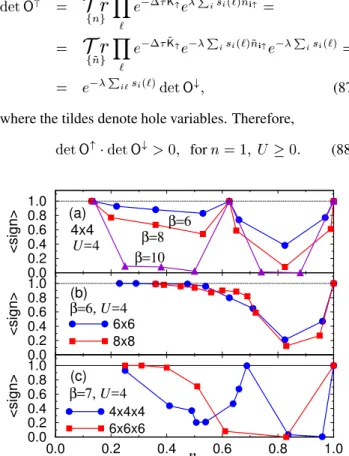
Figure 1. The average sign of the product of fermionic determi-nants as a function of band filling, for the Hubbard model with
U =4: (a)44square lattice, for inverse temperatures =6 (circles), 8 (squares), and 10 (triangles); adapted from Refs. [8] and [13]. (b)66(circles) and88(squares) square lattice, for fixed inverse temperature,=6; adapted from Ref. [13]. (c)
444(circles) and666(squares) simple cubic lattice, for fixed inverse temperature,=7. Lines are guides to the eye in all cases.
For the attractive Hubbard model, the lack of -dependence in the discrete HS transformation [see the com-ments below Eq. (18)] leads to O
"
(fsg) O #
(fsg), so that the product of determinants is positivefor all fillings. Similar arguments apply to show that the fermionic determi-nant is always positive for the Holstein model for electron-phonon interactions [40,41].
as a sum over configurations, fsg, of the ‘Boltzmann weight’, p() detO
"
(fsg)detO #
(fsg). If we write p() = s()jp()j, wheres() = 1 to keep track of the sign ofp(), the average of a quantitityAcan be replaced by an average weighted byjp()jas follows
hAi p
= P
p()A() P
p()
= P
jp()js()A() P
jp()js() =
= [
P
jp()js()A()℄= P
jp()j
[ P
jp()js()℄= P
jp()j
=
= P
p
0
()[s()A()℄ P
p
0
()[s()℄
hsAi p
0
hsi p
0
; (89)
wherep 0
() jp()j. Therefore, if the absolute value of p()is used as the Boltzmann weight, one pays the price of having to divide the averages by theaverage sign of the product of fermionic determinants,hsignihsi
p
0. When-ever this quantity is small, much longer runs (in comparison to the cases in whichhsigni'1) are necessary to compen-sate the strong fluctuations inhAi
p. Indeed, from Eq. (7) we can estimate that the runs need to be stretched by a factor on the order ofhsigni
2
in order to obtain the same quality of data as forhsigni'1.
In Fig. 1(a), we show the behaviour ofhsignias a func-tion of band filling, for the Hubbard model on a44square lattice withU =4, and for three different temperatures. One sees that, away fromn = 1, hsigniis only well behaved at certain fillings, corresponding to ‘closed-shell’ configura-tions; i.e., those such that the ground state of the otherwise free system is non-degenerate [13]. For the case at hand, the special fillings are 2 and 10 fermions on 44 sites, leading ton=0:125and 0.625, respectively. At any given non-special filling,hsignideteriorates steadily as the tem-perature decreases, rendering the simulations inpractical in some cases. Further, Fig. 1(b) shows that for a given tem-perature, the dip inhsignigets deeper as the system size increases. One should note, however, that the position of the global minimum is roughly independent of the system size, which, for fillings away from the dip, allows one to safely monitor size effects on the calculated properties. In this re-spect, the three-dimensional model is much less friendly, as shown in Fig. 1(c): for0:3.n<1,hsigniis never larger than 0.5 at the same filling for both system sizes.
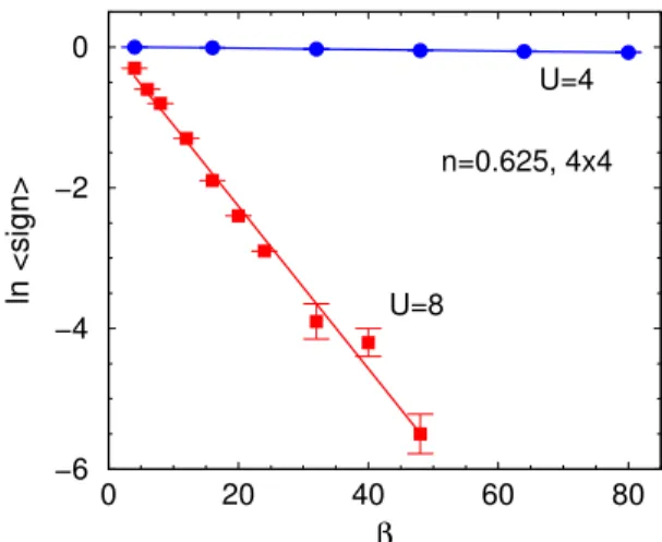
It is also instructive to discuss the dependence ofhsigni with temperature, keeping fixed both the system size and the band filling. In Fig. 2 we showlnhsignivs.for the44 lattice at the closed-shell fillingn=0:625. (Actually, these data have been obtained in Ref. [40] by means of a ground state algorithm, but they follow a trend similar to those ob-tained from the determinantal algorithm discussed here.) As U increases, the sign deteriorates even for this special fill-ing. For other fillings the average sign also decreases with U, and confirms the general expectation [40] that
hsignie Ns
; (90)
wheredepends onnandU. While for a givenn, the de-pendence ofonUis monotonic, for a givenU,is smaller
at the special fillings than elsewhere.
The fundamental question then is how to prevent, or at least to minimize, this minus-sign problem. While one could be tempted to attribute the presence of negative-weight con-figurations to the special choice of Hubbard-Stratonovich transformations (HST’s) used, it has been argued [42] that even the most general forms of HST’s are unable to remove the sign problem. It therefore seems that the problem is of a more fundamental nature.
0 20 40 60 80
β −6
−4 −2 0
ln <sign>
n=0.625, 4x4 U=4
U=8
Figure 2. The logarithm of the average sign of the product of fermionic determinants as a function of inverse temperature, for the Hubbard model on a44square lattice withn=0:625, and for different values of the Coulomb repulsion:U =4(circles) and 8 (squares). Lines are fits through the data points. Adapted from Ref. [40].
In order to pinpoint the origin of the problem, let us change the notation slightly and write the partition function as
Z= X
S Tr
Y
B
(S
M )B
(S
M 1 )B
(S
1
); (91) where a generic HS configuration of the`-th time slice is now denoted by S
`
fs
1 (`);s
2
(`);s N
s
(`)g; the set S fS
1 ;S
2 ;S
M
gdefines acomplete pathin the space of HS fields. Instead of applying the HST to all time slices at once, one can apply it to each time slice in succession, and collect the contribution from a given HS configuration of the first`time slices into thepartial path[43],
P `
(fS 1
;S 2
;;S `
g)
Tr "
BBB Y
B
(S
` )B
(S
` 1 )B
(S
1 )
#
;
(92) where there areM `factors ofB e
H
which have not undergone a HST. Clearly,P
0
yet; it is therefore positive. When HS fields are introduced in the first time slice, a “shower” of2
N
s different values of P
1 emerges from P
0; see Fig. 3. Each subsequent intro-duction of HS fields leads to showers of2
Ns
values ofP ` emerging from each P
` 1. In Fig. 3, we only follow two representativepartial paths: the top one is always positive, while the bottom one hits the`-axis at some`
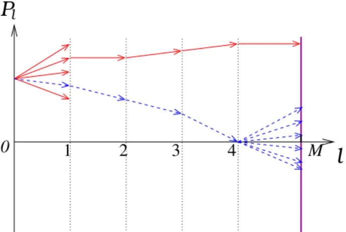
0. In the latter case, subsequent showers lead to both negative and positive values of the partial paths. According to the framework dis-cussed in Sec. 4, the simulations are carried out after per-forming the HST on all sites of all time slices. In the present context, this amounts to sampling solely the intersection of all possible paths with the vertical line at` =M; see Fig. 3. If one were able to sum overallHS configurations, we would find that the number of positiveP
M’s would exceed that of negativeP
M’s by an amount which, at low tempera-tures, would be exponentially small. Since in practice only a limited set of HS configurations is sampled, it is hardly sur-prising that we find instances in which configurations lead-ing to negative weights outnumber those leadlead-ing to positive weights. This perspective also helps us to understand why simply discarding those negative-weighted configurations is not correct: the overall contribution of the positive-weighted configurations would be overestimated in the ensemble av-erages.
4
P
ll
0
1
2
3
M
Figure 3. Schematic behaviour of partial paths (see text) as a func-tion of their length. Only two representative paths emerging from the “shower” at ` = 0are followed: one (full curve) leads to a positive contribution when it reaches ` = M, whereas the other (dashed curve) reachesP=0at some`0.
The analysis of partial paths is at the heart of a recent proposal [43] to solve the minus-sign problem. It is based on the fact that when a partial path touches the P = 0 axis, it leads to showers which, when summed over all sub-sequent HS fields, give a vanishing contribution; see Fig. 3. In other words, a replacement of allB’s in Eq. (92) by P
S `
0 +1
Q
B
(S
`0+1
) does not change the fact that P
` 0
=0. Therefore, if one is able to follow the ‘time’ evo-lution of the partial paths, and discard those that vanish at ` < M, only positive-weight configurations end up con-tributing at`=M. However, though very simple in princi-ple, this programme is actually quite hard to implement due
to the need to handle theBfactors without using a HS trans-formation. Zhang [43] suggested the use oftrialB’s, and preliminary results seem encouraging. Clearly, much more work is needed along these lines in order to fully assess the efficiency and robustness of the method.
Likewise, other recent and interesting proposals to deal with the minus sign problem need to be thoroughly scru-tinized. In the meron-cluster approach [44], HS fields are introduced in all sites as usual, but during the sampling process (1) the configurations are decomposed into clus-ters which can be flipped independently, and (2) a match-ing between positive- and negative-weighted configurations is sought; see Ref. [44] for details, and Ref. [45] for another grouping strategy. Another approach [46], so far devised for the ground-state projector algorithm, consists of introducing a decision-making step to guide walkers to avoid configura-tions leading to zero weight; it would be worth examining whether the ideas behind this adaptive sampling approach could also be applied to the finite temperature algorithm. In this respect it should be noted that Zhang’s approach is closely related to the Constrained Path Quantum Monte Carlo[47], in which the ground-state energy and correlation functions are obtained by eliminating configurations giving rise to negative overlaps with a trial state.
In summary, at the time of this writing, QMC simula-tions are still plagued by the negative-sign problem. Many ideas to solve this problem have been tested over the years, and they require either some bias (through resorting to trial states) or quite intricate algorithms (which render simula-tions of moderately large systems at low temperatures pro-hibitive in terms of CPU time), or both. We hope these re-cent proposals can be implemented in an optimized way.
6
Instabilities at low temperatures
When the framework discussed so far is implemented into actual simulations, one faces yet another problem, namely, the fact that the calculation of Green’s functions becomes unstable at low temperatures. As mentioned in the para-graph below Eq. (52), the Green’s functions can be iterated for about~
`10time slices, after which they have to be cal-culated from scratch. However, as the temperature is low-ered,i.e.,for &4,
~
`must be decreased due to large errors in the iterated Green’s function (as compared with the one calculated from scratch). One soon reaches the situation in which the Green’s function has to be calculated from scratch at every time slice (i.e., ~
`=1). It should be noted that this corruption only occurs as one iterates from one time slice to another, and not in the updating stage within a given time slice [13]. Worse still is the fact that as the temperature is lowered further, the Green’s function cannot even be cal-culated from scratch, sinceO
= 1+A
(`) becomes so ill-conditioned that it cannot be inverted by simple methods. For instance, in two dimensions and forU =0, the eigen-values ofO
range between1ande 4
eigenvalues ofO
to grow exponentially withM, thus be-coming singular at low temperatures.
Having located the problem, two solutions have been proposed, which we discuss in turn.
A. The Space-time Formulation
The approach used so far can be termed as aspace for-mulation, since the basic ingredient, the Green’s function [or, equivalently, the matricesA
andO
, c..f.Eqs. (26), (38), and (39)] is anN
s
N
s matrix. However, within a field-theoretic framework, if space is discretized before in-tegrating out the fermionic degrees of freedom [9], the ma-tricesO
are blown up to
^ O
= 0
B B B B B
1 0 0 0 B
M B
1
1 0 0 0
0 B
2
1 0 0
..
. ... ... ..
. ...
0 0 0 B
M 1
1 1
C C C C C A
; (93)
which is an (N s
M)(N s
M) matrix (since each of the MMentries is itself anN
s N
smatrix); one still has [9] det
^ O
=det[1+B M
B 1
℄; (94)
as in Eq. (23), and
Z=
1
2
L d
M
Tr
fsg det
^ O "
(fsg)det ^ O #
(fsg): (95)
Taking the inverse of ^ O
yields immediately the space-time Green’s function matrix,
^ g
= h
^ O
i 1
: (96)
This space-time formulation has the advantage of shrinking the range of eigenvalues of ^
O
: the ratio between its largest and smallest eigenvalues now grows only linearly withM, thus becoming numerically stable [12]. Though this approach has been extremely useful in the study of mag-netic impurities [47], it does slow down the simulations when applied to the usual Hubbard model [34]. Indeed, dealing with(N
s
M)(N s
M)Green’s functions would re-quire(N
s M)
2
operations per update,N 3 s
M 2
operations per time slice, and, finally,(N
s M)
3
operations per sweep of the space-time lattice. Sweeping through the space-time lattice with^g
is then a factor ofM 2
slower than sweeping with g
.
A solution of compromise between these two formula-tions was proposed by Hirsch [12]. Instead of using one time slice as a new entry in ^
O
[Eq. (93)], we collapseM 0
<M time slices into a new entry. That is, by takingM
0
M=p, withpan integer, one now deals with(N
s p)(N
s
p) matri-ces of the form
^ O M0
(1)= 0
B B B B B
1 0 0 0 B
pM0
B
(p 1)M0+1 B
M0
B M0 1
B 1
1 0 0 0
0 B
2M
0 B
M
0 +1
1 0 0
..
. ... ...
..
. ...
0 0 0 B
(p 1)M0
B
(p 2)M0+1
1
1
C C C C C A ;
(97) in terms of which the partition function is calculated as in Eq. (95). The label 1 of ^
O M
0
indicates that the product of B’s start at the first time slice of each of thepgroupings. As a consequence, the time-dependent Green’s function sub-matrices, G
(`
1 ;`
2
), connecting the first time slice of each grouping with either itself or with the first time slice of subsequent groupings, are readily given by [12]
h ^ O M0
(1) i
1 ^g
M0
(1)= 0
B B B
G(1;1) G(1;M
0
+1) G(1;(p 1)M
0 +1)
G(M 0
+1;1) G(M
0 +1;M
0
+1) G(M
0
+1;(p 1)M 0
+1) ..
. ...
.. . G((p 1)M
0
+1;1) G((p 1)M 0
+1;M 0
+1) G((p 1)M 0
+1;(p 1)M 0
+1) 1
C C C A ;
(98) d
where the spin indices inGhave been omitted for simplic-ity. The Green’s functions connecting the`-th time slices of thepgroupings are similarly obtained from the inversion of
^ O
M0
(`), which, in turn, is obtained by increasing all time indices of theB’s in Eq. (97) by` 1.
In the course of simulations, one starts with the
^ g
M0
(2)through [12] G(`
1 +1;`
2
+1)=B `
1 G(`
1 ;`
2 )B
1 `2
: (99)
We then sweep through all sites of the second time slice of each of thepgroupings, and so forth, until all time slices are swept. Note that since Eq. (99) is only usedM
0 times (as opposed toMtimes) it does not lead to instabilities forM
0 small enough.
Each Green’s function update with Eq. (51) requires
(N
s p)
2
operations; sweeping through all spatial sites of one time slice in each of every pgroupings therefore re-quires(N
s p)
3
operations. Since there areM
0 slices on each grouping, one has, finally, a total ofN
3 s
Mp 2
opera-tions per sweep, which sets the scale of computer time; this should be compared withN
3 s
M for the original implemen-tation, and(N
s M)
3
for the impurity algorithm. The strategy is then to keepM
0
20and letpincrease as the tempera-ture is lowered. With this algorithm, values of20 30 have been achieved in many studies of the Hubbard model; see, e.g., Refs. [25,35,37,21,33,48,49,50,29]. It should also be mentioned that since the unequal-time Green’s function is calculated at each step, this space-time formulation is es-pecially convenient when one needs frequency-dependent quantities [37].
B. Matrix-decomposition stabilization
Let us assume thatM 0of the
Bmatrices can be multi-plied without deteriorating the accuracy. One then defines [13,14]
~ A 1
(`)B `+M0
B `+M0 1
B `
; (100)
which, by Gram-Schmidt orthogonalization, can be decom-posed into
~ A 1
(`)=U 1 D
1 R
1
; (101)
where U
1 is a well-conditioned orthogonal matrix, D
1 is a diagonal matrix with a wide spectrum (in the sense dis-cussed at the beginning of the Section), andR
1is a right tri-angular matrix which turns out to be well-conditioned [13].
Using the fact thatU
1 is well-conditioned, we can mul-tiply it by another group ofM
0matrices, Q=B
`+2M0
B `+2M0 1
B `+M0+1
U 1
; (102)
without compromising the accuracy. We then form the prod-uct
Q 0
=QD 1
; (103)
which amounts to a simple rescaling of the columns, without jeopardizing the stability for the subsequent decomposition as
Q 0
=U 2 D
2 ~ R 2
; (104)
where the matricesU 2,
D 2, and
~ R
2 satisfy the same condi-tions as in the first step, Eq. (101). WithR
2
~ R 2 R
2, we conclude the second step with
~ A 2
(`)=U 2 D
2 R
2
: (105)
This process is then repeatedp =M=M
0 times, to finally recover Eq. (39), in the form [13]
A
(`)= ~ A p
=U p D
p R
p
: (106)
The equal-time Green’s function is therefore calculated through Eq. (38), as before, but care must be taken when adding the identity matrix toA, since the latter involves the wide-spectrum matrixD
p. One therefore writes 1=U
p
U p
1 R
p
R p
1
; (107)
so that the inverse of Eq. (38) becomes [g
(`)℄
1 =U
p P
R
p
; (108)
with
P
=
U p
1
R p
1 +D
p
: (109)
We now apply another decomposition to P, the result of which is multiplied to the left byU
p, and to the right by R
p, in order to express the Green’s function in the form [13] [g
(`)℄
1 =U
D
R
: (110)
In the course of simulations, one proceeds exactly as in Sec. 4, by updating the Green’s function through iterations, which takes up N
3 s
M operations. Again, the iteration from one time slice to another is limited to about ~
` time slices, and it turns out that a significant fraction of the com-puter time is spent in calculating the Green’s function from scratch. Indeed, a freshg is calculatedM=
~
` times, each of which involvingpdecompositions, each of which taking aboutN
3
s operations. Therefore, taking ~
` p, the dom-inant scale of computer time is N
3 s p
2
instead, which is about a factor ofM faster than the space-time algorithm, though without the bonus of the unequal-time Green’s func-tions. This matrix decomposition algorithm has also been efficiently applied to several studies of the Hubbard model, and values of 20 30have been easily achieved; see, e.g.,Refs. [13,22,40,32,36,37,38,39,51].
7
Conclusions
We have reviewed the Determinantal Quantum Monte Carlo technique for fermionic problems. Since the seminal pro-posal by Blankenbecler, Scalapino, and Sugar [9], over twenty years ago, this method has evolved tremendously. Stabilization techniques allowed the calculation of a variety of quantities at very low temperatures, but the minus-sign problem still plagues the simulations, restricting a complete analysis over a wide range of band fillings and coupling con-stants. In this respect, it should be mentioned that other im-plementations of QMC, such as ground-state algorithms (see Ref. [8]), also suffer from this minus-sign problem. An effi-cient solution of this problem would be a major contribution to the field.
of other models, such as the extended Hubbard model [52], the Anderson impurity model [47], and the Kondo lattice model [53]. The first applications of QMC simulations to disordered systems have appeared only recently; see, e.g., Refs. [38,39]. With the ever increasing power of personal computers and workstations, one can foresee that many properties of these and of more ellaborate and realistic mod-els will soon be elucidated.
Acknowledgments
The author is grateful to F. C. Alcaraz and S. R. A. Salinas for the invitation to lecture at the 2002 Brazilian School on Statistical Mechanics, and for the constant en-couragement to write these notes. Financial support from the Brazilian agencies CNPq, FAPERJ, and Minist´erio de Ciˆencia e Tecnologia, through the Millenium Institute for Nanosciences, is also gratefully acknowledged.
A
Grouping products of exponentials
One frequently needs to group products of exponentials into a single exponential. Here we establish a crucial result for our current purposes: the product of bilinear forms can be grouped into a single exponential of a bilinear form.
To show this result [8], let the generic Hamiltonian be expressed as (we omit spin indices)
H= X
i;j
y i h
ij
j
; (111)
wherehis a matrix representation of the operatorH. The ‘time’ evolution of Heisenberg operators [c.f.,Eq. (36)], sat-isfies a differential equation, whose solution can be found to be
y i
()= X
i
e h
ij
y i
: (112)
If we now take the linear combination
y
= X
i B
i
y i
; (113)
we see that
y
() =
X
i X
j
e h
ij B
j
y i
=
X
i ~ B i
y i
; (114)
where the last passage has been used as the definition of ~ B. Now we introduce the product over time slices, through
U
Y
` e
H(`)
; (115)
so that theh’s now acquire`-labels, and we have
U y
= X
i X
j "
Y
` e
h(`) #
ji B
j
y i
U =
XX
h e
~ h i
ji B
j
y i
U; (116)
where, again, the last passage has been used to define~ h. We can then write
U y
U 1
= X
i X
j h
e
~ h i
ji B
j
y i
; (117)
so thatU indeed behaves as a single exponential of the ef-fective bilinear Hamiltonian ~
H, whose elements are defined by
" Y
` e
h(`) #
ij =
h e
~ h i
ij
: (118)
B
Tracing
out
exponentials
of
fermion operators
We now use the results of App. A to show that the trace over the fermionic degrees of freedom can be expressed in the form of a determinant. Given that ~
His bilinear in fermion operators, it can be straightforwardly diagonalized [9,11,8,14]:
~ H=
X
"
y
; (119)
where, for completeness, the relations between ‘old’ and ‘new’ fermion operators are
= X
i hjii
i
; (120)
and
y
= X
i hiji
y i
; (121)
the inverse relations are
i
= X
hiji
; (122)
and
y i
= X
hjii
y
: (123)
Given the diagonal form, the fermion trace is then im-mediately given by
Tr Y
` e
H(`)
= Tre
~ H
=
= Tre
P
" y
=
= Tr Y
e
" y
=
= Y
1+e
"
=
= det h
1+e
~ H i
=
= det "
1+ Y
` e
h(`) #