Braz. J. Phys. vol.36 número4A

The Spreading Width Calculation of Giant Resonances with a Semi-Microscopic Approach

T. N. Leite1,2 and N. Teruya2 1 _{Colegiado de Engenharia Civil}

Fund. Universidade Federal do Vale do S ˜ao Francisco C.P. 309, 48900-000 Juazeiro, BA, Brazil.

2 _{Departamento de F´ısica, Universidade Federal da Para´ıba}

C.P. 5008, 58051-970 Jo˜ao Pessoa, PB, Brazil

Received on 26 August, 2006

We have proposed a semi-microscopic approach to calculate the two particles - two holes (2p−2h) spreading width of giant resonances. Our proposal has been based in a hybrid method that implements the statistical multistep compound theory of Feshbach, Kerman and Koonin (FKK), widely and successful used in nuclear reactions mechanisms, in order to include relevant informations about the microscopic structure obtained by the Random Phase Approximation (RPA) calculations. This method is an approximative calculation to avoid the intrinsic numerical difficulties of those microscopic calculations that incorporate more complex structure than one particle - one hole (1p−1h) excitations. Unlike the reaction context, the residual interaction was adjusted inRPAcalculation to reproduce the lowest energy levels of the studied nuclei. The feasibility and the efficiency of the approach has been tested in giant dipole resonances in208Pband neutron-rich calcium isotopes,48Caand 60_Ca.

Keywords: Giant Resonance, Statistical Multistep Compound Theory, Random Phase Approximation, Spreading Width.

I. INTRODUCTION

The calculation of the decay widths of the giant resonances (GR) in nuclei supplies a measure of the fragmentation degree of their decay mechanisms. These mechanisms have taken a special attention in nuclear physics research [1, 2] since the discovered of those highly collective nuclear excitations. The GR’s energy is located above the threshold of particle emis-sion and its classification in terms of the direct and statisti-cal decay modes has been a permanent discussion in the lit-erature. The competition between these decay modes can be formulated through an evolution chain in a particle-hole ba-sis, which allows the decomposition of the total width (Γ) in two components: the escape width (Γ↑_{), that couples directly}

one particle to the continuum, and the spreading width (Γ↓_),

due to the coupling to internal degrees of freedom like low-lying surface modes and 2p₋2h excitations. In this sense, the total width can be written asΓ=Γ↑_+Γ↓_{. The study of}

the competition between these decay modes has always mo-tivated the development of methods of calculations of these widths, bringing new insights to the understanding of the res-onances microscopic structure. The Random Phase Approx-imation (RPA) has been reaching a lot of theoretical success to describe theGRmicroscopically as a coherent superposi-tion of particle-hole excitasuperposi-tions. Various different versions of this theory have been developed to treat the escape process by considering the coupling of 1p₋1hexcitations to the contin-uum [3–10]. Beside these efforts the study of the spreading process also had their improvements by extending the 1p₋1h basis in order to include 2p₋2hexcitations [11–13] in aRPA -like treatment, named secondRPA. However, in face to the enormous dimensions of the matrices that describe the second RPA these calculations become impracticable, mainly when applied to the heavy nuclei, requiring a long time of numeri-cal computation. To outline these intrinsic numerinumeri-cal difficul-ties some approximated methods were developed to calculate

the widths related with more complex structure than 1p₋1h [14–19].

In Ref. [20], we have analysed the structure of the isovec-tor dipole resonance in neutron-rich calcium isotope, 60Ca, by using a previous version of the continuumRPAapproach [10], which was modified to take into account the differences among the neutron and proton radii in nuclei with neutron ex-cess. We have observed a small escape width of the giant di-pole resonance (GDR) in this nucleus, indicating that the more complicated excitations than 1p₋1h should also be impor-tant for the description of its microscopic structure. Recently, we have applied the same method for the analyses of the di-rect decay mode of isoscalar giant dipole resonances (ISGDR) in208Pb[21], whose new studies have been stimulating the improvements of the structure calculations largely around the ISGDR[19, 22–27].

The purpose of this paper is to complete the investiga-tion about the GRdecay mechanisms, and to present a fea-sible scheme to calculate theGR’s spreading width. There-fore, we present a new formulation of an approximated semi-microscopic method, based in the statistical Multi-Step Compound Theory (MSC) of Feshbach, Kerman and Koonin (FKK) [28] in connection with theRPA calculations. This procedure overcomes the inherent numerical difficulties in the secondRPAto investigate the 2p₋2hstructure, and also al-lows to include in theFKK approach the same residual in-teraction used in theRPAcalculations. This fact is an impor-tant point regarding the management of the residual interac-tion, what in our proposal it is made in consonance with the RPAcalculations, maintaining a cohesion between both the approaches. This method has been tested in giant dipole reso-nances in208Pband neutron-rich calcium isotopes,48Caand 60_Ca.

of XXVII Workshop on Nuclear Physics in Brazil (2004), published in special issue of Brazilian Journal of Physics [29]. In the Sect. II of this paper, we present the semi-micorscopical approach used in the spreading width calcula-tion. The results are discussed in the Sect. III.

II. THE SEMI-MICROSCOPIC APPROACH

In order to perform the calculation of the spreading width, we can use the Statistical Multi-Step Compound Theory (MSC) of Feshbach, Kerman and Koonin (FKK) [28]. In this approach, the excitation of theGR takes place in a number of stages, the particle emission is allowed in anyone of them. Each stage is represented by a level of complexity, which is characterized by the number of particle-hole pairs that are ex-cited by an external field: the first stage has 1p₋1h config-uration, the second one has 2p₋2hconfiguration and so on, until the compound nucleus formation [30].

According to this formalism, the average total widthΓnJ for each stagen(np₋nh) with angular momentumJis given by the sum of the escape contributionΓ↑_nJ, due to the con-tinuum coupling, and the spreading contributionΓ↓_nJ, due to the transition for more complex stages. The spreading width for thenth stage, for a excitation energyE, is given by

Γ↓_nJn+1(E)=2π|H J n,n+1|2

Dn+1J

(1)

where|H_n,nJ _+1|2is the mean square matrix element of inter-action that couples thenandn+1 stages with total angular momentum J, and Dn+1J is the average spacing of levels in the(n+1)st stage coupling to the total angular momen-tum J. The average process is performed over initial states and summed over final states by considering the particle-hole level densityρph(E,J)with energyEand angular momentum

J.

By assuming an energy and angular momentum factoriza-tion of the state densityρph(E,J),

ρph(E,J) =ω(p,h,E)Rn(J), (2)

the spreading width is written as [28]:

Γ↓_nJn+1(E)=X_{n J}↓n+1Y_n↓n+1(E) (3) TheXfunction contains the angular momentum structure in-cluded in the particle-particle two-body interaction and the spin distribution of the single particle levels. TheY function contains all the dependence on excitation energy originating from the final state density, the particle-hole distinguishabil-ity, and describes the available phase space for the transition.

In order to calculate theX function we are considering the diagrammatic representation for the process with the addi-tional creation of a particle-hole pair (see FIG. 1). By per-forming the average process with a general two-body interac-tion, we have obtained

J

S j3

❆ ❆ ❆ ❆

❑

j

✁✁ ✁✁ ✕

Q

❆ ❆ ❆ ❆

❑

j1

✁✁ ✁✁ ☛

j2

j4

J

FIG. 1: Diagram with the angular momentum coupling [30] used in theX function computation for the process which one particle-hole pair is created. As we do not considered the distinguishability between particle (up arrow) and hole (down arrow), the two-body interaction (dashed line) is particle-particle type.

X_nJ↓(n+1) = 2π

_∑

jQ j4j3

R1(j)R1(Q)RN−1(j4) RN(J)

(2j3+1)

(2Q+1)∆(QJ j4)

∑

j1j2

R1(j1)R1(j2) ({j1j2}j3|V|{Q j}j3)

2 (4)

where

RN(J) =

(2J+1) π12_N32σ3

exp(−(J+

1 2)2

Nσ2 ) (5)

is the angular momentum distribution of the single-particle levels with a spin cut-off parameter

σ=

_√ 12 45π

A53

g 1

2

, (6)

related to the single-particle spacingg, and

N=

p+h=2n,Neven

p+h+1=2n+1,Nodd (7) is the number of the excited particle-hole pairs (number of excitons). The function∆(jajbjc)guarantees the angular mo-mentum conservation, i.e.,∆(jajbjc) =1 if|−→ja−−→jb| ≤jc≤ |−→ja+−→jb|or zero otherwise.

The computation of theYfunction is similar to that of theX. In this case, we have considered the state densities of the ini-tial and final hole configurations. Due to the particle-hole distinguishability, there are two spreading process, cor-responding to a particle or a hole interacting with a bound nucleon, exciting an additional particle-hole pair (see FIG. 2). So we have

(a)

✁✁ ✁✁ ✕ ❆ ❆ ❆ ❆ ❑ ❆ ❆ ❆ ❆ ❑ ✁✁ ✁✁ ☛

Energy

E

−

Z

Energy

Z

Total Energy =

_E

(b)

❆ ❆ ❆ ❆ ❯ ✁✁ ✁✁ ☛ ❆ ❆ ❆ ❆ ❑ ✁✁ ✁✁ ☛

Energy

E

−

Z

Energy

Z

FIG. 2: Diagram with the energy conservation [30] in order to calcu-late theYfunction considering the two possible processes to excite a particle-hole pair, taking account the particle-hole distinguishability.

with

aYn↓n+1(E) =

E

0

ω(1,0,E₋z)ω(p−1,h,z)

ω(p,h,E) ω(2,1,E−z)dz (9)

bYn↓n+1(E) =

E

0

ω(0,1,E₋z)ω(p,h₋1,z)

ω(p,h,E) ω(1,2,E−z)dz (10) wherezis the core energy.

The form of the particle-hole state density considered is that proposed by Oblozinsky [31]:

ω(p,h,E) = g

N

p!h!(N−1)! p

∑

i=0 h

∑

k=0 (−1)i+k

_p i

_h k

×Θ(E−αph−iB−kF)

×E₋Aph−iB−kFN−1 (11) whereBandF is the binding and Fermi energy, respectively; the step functionΘ(x)is unity forx>0 and zero otherwise; αph is the minimum energy needed to excite p-particles and

h-holes satisfying the Pauli principle and is given by

αph= 1 2

p2+p+h2₋h g

, (12)

and the quantity

Aph= 1 4

_p2_+p+h2_−3h g

, (13)

accounts for Pauli blocking. In Ref. [28] the density of particle(hole) states is derived from the equidistant single-particle model, resulting in a n-stageYn(E) function with a direct dependence onE2_{. Therefore, for resonances at} ener-gies far away from the nucleon binding energy (as in isoscalar GDR) this outcome is not a good option because the spread-ing width involves only intermediate bound states. This way, we use theYn(E)function proposed by Oblozinsky [31] where

the level density is obtained restricting the nucleons to bound states, limiting the energy dependence.

After this brief discussion about theFKK approach, we present some necessary modifications to connect it with the nuclear structure calculations likeRPA. The definition of the spreading width in Eq.(1) and the form as the density of states was written in Eq.(2) permits to factor the width in terms of the product of the functions X andY in Eq.(3), resulting a X function that does not depend on the excitation energyE. Thus, theX andY functions are calculated separately, result-ing in a complete uncouplresult-ing between the angular momentum of the excited particle-hole pairs and the energy where they are considered in the calculation of the width. This way, all 1p₋1hpairs are treated in the same foot in any energy, mak-ing the results to depend strongly on the particle-hole basis considered. On the other hand, inRPAapproach, the excita-tion probability of a specific particle-hole pair depends on the excitation energy and its angular momentum coupling. There-fore, since we have accounted a fairly complete 1p₋1hbasis in aRPAcalculation, the results do not undergo considerable alteration by including another more internal (or more exter-nal) single-particle level in the configuration basis, besides those already taken into account in the “fairly complete” basis. Nevertheless, as in theFKKapproach the constraint between the energy and angular momentum of the single-particle level is broken, the spreading width calculation does not take ac-count these important microscopic informations about the oc-currence probability of each pair 1p₋1hon the energy of the GR.

In order to include these microscopic informations calcu-lated byRPA, to minimize the dependence with the 1p₋1h basis and the number of possible intermediate couplings, we have implemented some modifications in the original form [28] of theX function. The main modification consists in to take into account the excitation probability of each 1p₋1h pair that is accessed in the energy in which the calcula-tions are performed (this proposal is hereafter referred to as RPA+FKKapproach). This reformulatedXfunction is given by:

X_nJ↓(n+1)(E) =2π

_∑

jQ j4j3

P

Q jJ 4

R1(j)R1(Q)RN₋1(j4) RN(J) ×(₍2j3+1)

2Q+1)∆(QJ j4)

∑

_j

1j2

P

j3

j1j2R1(j1)R1(j2) ×({j1j2}j3|V|{Q j}j3)

2_L(E,E

2) (14)

where the inclusion of the factor

P

jJpjh controls the probability of accessing each 1p₋1hconfiguration, and also it minimizes the dependences with the 1p₋1hbasis and the number of j3 couplings. We have taken into account only phonons (j3) with energy smaller than the energy of particle threshold, as well as in the calculations based on the secondRPAversions [14–18]. The quantityL(E,E2p−2h)is a lorentzian type function,

L(E,E2p₋2h) =

η2 (E−E2p−2h)2+η2

withE2p−2h=εj+εj1−εj4−εj2(εis the energy of the

single-particle level). It simulates the energy denominator of the sec-ondRPAcalculation and gives a measurement of the fragmen-tation of theRPAsolution into 2p₋2hspace. Thus the acces-sibility of some single-particle level jmay be considered. We would like to emphasize that now the calculation ofX func-tion is performed in each excitafunc-tion energy (E) at theGR en-ergy position, and with the respective

P

Jjpjh andL(E,E2p−2h) factors.

We define the factors

P

Jjpjh as function of the 1p−1h for-wardRPAamplitudes (xJ_j

pjh):

P

Jjpjh=

NP|xJjpjh| 2

∑ jpjh(Γp≈0)

|xJ_j pjh|

2 , (16)

where Np is the number of bound (or with single-particle width too smaller thanGRwidth) 1p₋1hconfigurations cou-pling to−→J. TheRPAamplitudes are obtained by a diagonal-ization of the complex equation:

A B

−B ₋A

xm ym

=εm

xm ym

(17)

where

A_php′_h′= (εp−εh)δpp′δhh′+Vph′hp′;Bphp′h′ =Vpp′hh′ (18) and εp (εp=εp−1₂iΓp) are the complex energies of the single-particle resonances [32, 33]. The real part of the com-plex eigenvaluesεmgives the excitation energy (εm), and the imaginary part gives the escape width (Γ↑m) of the 1p−1h ex-citation mode (See Refs. [10] and [20] for more details).

The discrete single-particle energies were evaluated by solving the Schr¨odinger equation with Woods-Saxon poten-tial, including the centrifugal and Coulomb (as a uniformly charged sphere) terms. The positive single-particle energy and its respective width were calculated in a projection technique to continuum discretization approach discussed in Refs.[32, 33]. TheRPAcalculation was done by utilizing the Landau-Migdal residual interaction:

Vph(−→r1,−→r2) =C0[f(r1) +f′(r1)−→τ1· −→τ2+ +−σ1→· −→σ2g(r1) +g′(r1)−→τ1· −→τ2

]δ(−→r1− −→r2) (19) wheref,f′,gandg′are dimensionless and density dependent parameters:

F(r) =Fex+ (Fin−Fex)ξ(r). (20)

The set of the interaction parameters was adjusted to elimi-nate the spurious state 1− (see TABLE I) and to reproduce the first 3− excited state for each nucleus under consider-ation. Since the neutron and proton densities are too dif-ferent in nuclei with neutron excess, it is more appropri-ate to separappropri-ate the nucleon density into neutron and proton parts, ξ(r) = N

Aξν(r) + Z

Aξπ(r), where each part is given by

ξk(r) = 1

1+e(r−Rk)/ak , withk=ν(π)for neutron (proton) [20].

In this same sense, the radial single-particle orbits are rep-resented by harmonic oscillator radial wave functions with different size parameters for neutrons and protons, b2_{k ≈}

4

(3)43

r2 k(Xk)−

1

3 [20], wherer2_k≈3

5R2k+ 7

5π2a2k[34]. We have adopted the following criterion in order to choose the parameterηin Eq.(15):

η=ηm=min(

εm−εm−1

4 ,

εm+1−εm

4 ), (21)

whereεmare the energies obtained inRPAcalculation around the GR position. We have considered only RPA solutions (εm) that exhaust at least 1% fraction of the the Energy Weighted Sum Rule (EW SR). This criterion assure that we have considered only 2p₋2h poles, E2p₋2h, in the neighborhood of solutionεm, i.e., the common area among the lorentzianL(εm,E2p−2h)and its neighboring lorentzians,

L(εm−1,E2p−2h)andL(εm+1,E2p−2h), is small. Then we have not taken account the 2p₋2h poles that are lied out of the neighborhood ofεm(energy interval:[εm−1+2η,εm+1−2η]). This way, variousRPApeaks can be superposing in the en-ergy interval aroundGR, and the medium values of the energy and width are obtained through an average process over the involved peaks. These medium values are calculated by per-forming the weighted average:

a=∑mPmam ∑mPm

, (22)

whereamrepresents the value to be averaged and the weights,

Pm, are the intensities of each peak relative to the fraction of

EW SRthat they exhaust in the specific energy interval. For an arbitrary energy interval[EI,EF]we get the definitions:

Pm(%)≡100× EF

EI S

m

F(E)E dE

EW SR , (23)

where the strength functionSF(E)is written as

SF(E) =

∑

m

S_Fm(E), (24)

and

EW SR=

EF

EI

SF(E)E dE. (25) In order to calculate the the strength function SF(E) we have assuned the particle-hole matrix element of the 1-body dipole operator (F_λ=1) as

F₁T_M=1=ekrY1M (26) for isovector (T =1) electric dipole transition, whereekis the nucleon effective charge, i.e.,eν(π)=−eZA (

eN A), and

Another point that deserves a special attention is the part that deals with the residual interaction used in the calculation. The consistency of theRPA+FKKapproach is guaranteed by using the same Landau-Migdal interaction to diagonalize the RPAequations and to compute theXfunction. However, in the FKK calculations [28, 30, 37, 38], the two-body interaction was assumed to be the simplest zero-range form

V(−→r1,−→r2) =V0( 4 3πr

3

0)δ(−→r1− −→r2), (28) where the strength of the interaction,V0, is a free parameter. It is frequently adjusted in order to reproduce some experimen-tal data that can be calculated by the formalism. There is no standard procedure to adjustV0, and it is controlled in each specific calculation. This makes possible many other differ-ent forms of getting such adjustmdiffer-ents, what could cause great variations on theV0values. In this context, the studies per-formed by R. Bonetti and L. Colombo [37] have showed that V0increases when more realistic ingredients are included in the computation of matrix element of the interaction. In a se-ries of calculations to reproduce the widths of precompound and compound nuclearr-stage, extracted from the experimen-tal data about27_Al(3_{He,p)reaction, they used different details} concerning the interaction, wave functions and level densities, and they verified the occurrence of great variations in theV0 values. In another way, distinct procedures were adopted to fit the experimental data in the Refs.[28, 30, 38] to treat different nuclear reactions. The varied forms to control the parameters of the residual interaction, as well as the management ofV0, seem to be a consequence of the difficulty to establish more general criteria to guide such adjustments.

In our proposal we have been adapting theFKKformalism to be applied in consonance with theRPAapproach. Proceed-ing this way, the parameters of the residual interaction had been adjusted at level of the RPA calculation in a standard way, in order to reproduce the excited states with the lowest energies and to eliminate the spurious solution at zero energy. Thus, the results for theGRare obtained as consequence of this parametrization. Soon after, this same set of parameters was used to calculate the spreading width. This procedure is taken to keep the coherence between these two types of calcu-lations for escape and spreading widths. In this sense, we do not have total freedom to choose the parameters, and we may interpret that the adjustments of a free parameter likeV0can accommodate some details that should be part of the calcula-tions. This statement becomes more evident when we write the squared matrix element of Eq.(14) in the following form:

j1j2;j3|V|Q j;j3 2

=

P

Q jJ 4

P

j3

j1j2(j1j2;j3|V|Q j;j3)

2

×L(εm,E2p−2h), (29)

with V in the form given by the expression (28). Thus, the nuclear structure effects displayed by

P

J

Q j4,

P

j3 j1j2 and

L(εm,E2p−2h)quantities could be hidden behind the adjust-ments ofV0.

TABLE I: Parameters of Landau-Migdal residual interaction.

Nucl. C0(MeV f m3) fin fex f′in f′ex g g′ 208_{Pb 368.75 0.200 −1.474 1.5 1.5 0.635 0.70}

48_{Ca 300.0 −0.002 −1.282 0.76 2.30 0.05 0.94} 60_{Ca 300.0 −0.002 −2.100 0.76 2.30 0.51 0.70}

TABLE II: Parameters of Fermi distribution and harmonic oscillator radial wavefunctions.

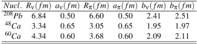
Nucl. Rν(f m) aν(f m) Rπ(f m) aπ(f m) bν(f m) bπ(f m)

208_{Pb 6.84 0.50 6.60 0.50 2.41 2.51} 48_{Ca 3.34 0.65 3.05 0.65 1.95 1.97} 60_{Ca 4.34 0.60 3.68 0.60 2.09 2.11}

III. RESULTS AND DISCUSSIONS

In this section we shall present the results for spreading widths for giant dipole resonances in208_Pband48,60_Ca nu-cleus. The set of parameters of residual interaction and har-monic oscillator radial wave function are given in TABLES I and II, respectively.

In the calculation of the spreading width we have taken into account the contributions of the intermediate phonons with multipole j3≤6, natural parity and energy smaller than the neutron separation energySn. The features of these low-lying modes are obtained by the continuumRPAdescribed in Ref [20]. This procedure is similar to others microscopic calcu-lations which considering the coupling to low-lying phonons [14–18]. Our results forGRwidths are summarized in TABLE III. The comparison with the experimental data was showed a quite reasonable agreement.

The first application test refers to the spreading width cal-culation of the isovectorGDRin208Pb. The experimental data get this resonance located around 13.5MeV with a total width of 4.0MeV [39]. The decay of this resonance in heavy nu-cleus is broadly dominated by the statistical mechanism, being compatible with a small direct neutron branching ratio. Our calculation gets a medium energy around of 10.8 MeV with a null escape width and a spreading width (Γ↓_=4.4MeV)

com-TABLE III: Summarized results.

Nucleus Mode Γ↑_{(MeV) Γ}↓_(MeV)

208_{Pb IVGDR 0.00 4.4}

ISGDR 2.67 3.3

48_{Ca IVGDR 0.13 4.3}

60_{Ca IVGDR 0.56 0.0}

Experimental values

E(MeV) Γ(MeV)

208_{Pb IVGDR 13.5 4.0[39]} ISGDR 20−23 2.5−10[22–24, 26] 48_{Ca IVGDR 19.9 7.0[44]}

posed by the presence of various narrow peaks superposing to exhaust about 82% of the EW SR between 20₋30MeV. These peaks are mainly composed by 3hωtransitions involv-ing the neutrons and protons of the externals shells. The en-ergy and escape width of this resonance were evaluated by performing a weighted average on the energies and widths of the peaks that compose it, the weights being the intensities of each peak relative to the 82% of theEW SRthat they exhaust. The centroid was calculated at 24.4MeV with an average es-cape width of 2.7MeV. Then, making use of these results for ISGDRin208Pb, provided by theRPAcalculations, we pro-ceed the calculation of the spreading width and we obtained

Γ↓_{=3.3MeV, resulting a total widthΓ=6.0MeV. The}

result of our escape width is larger than the value of 1.9MeV encountered by another calculation of continuum RPA[43], while our calculated spreading width is in agreement with the fits from Ref.[26], and also, with the value of 3.2MeV used in the analysis of the Ref.[43].

The others results refer to the analyses of the decay mecha-nisms of the isovector giant dipole resonances in neutron-rich calcium isotopes,48Caand60Ca. Experimentally, the isovec-torGDR in48Ca is localized around 19.5 MeV with width of 7.0MeV [44]. We have found about 97% of theEW SR between 10 and 21MeV by performing ourRPAcalculation, with two peaks exhausting 47% of theEW SRaround 20MeV. The mean energy is about 15.6MeVwith a very small escape width:Γ↑_{≈130keV, reflecting the narrow single-particles}

widths. This result is in disagreement with the Strauch et. al. estimates [45] which have given about 40% of direct neu-tron escape forGDRdecay in this nucleus. This large fraction was deduced by comparison of the residual nucleus excitation spectrum (47Ca), which was measured in48Ca(e,e′n) reac-tion, with the statistical model calculations. On the contrary, our result for spreading width (Γ↓_{=4.3MeV) is in good}

agreement with the statistical analysis performed in this ex-perimental work [45], which is compatible with 60% of the total width. With relation to 60Ca, the calculated spreading width in the isovectorGDRregion, around 15MeV, for this nucleus is very small, even considering many low-lying en-ergy phonons. This fact reinforce the statement which the two or more neutron escape should be important forGDRdecay in60Ca[20]. The spreading is small because there are few accessible intermediaries bound 1p₋1hpairs.

The widths summarized in TABLE III can assist us to make

a measure of the competition among the direct and statisti-cal decay mechanisms, for so much, we define the direct de-cay branching ratio asb↑=Γ↑_{/Γand the statistical}

branch-ing asb↓=1−b↑, whereΓ=Γ↑_+Γ↓_{is the total width. The}

branching ratios should be understood as reference values that indicate the degree of fragmentation of the giant resonances. Thus, the null escape width forIV GDRin208Pbrepresents the largest domain of the statistical decay (b↓_≃1) as it happens in heavy nuclei [40]. In a different way, the results for isoscalar E1 in208_{Pbindicate that this excitation mode should have a} strong fragmentation of its microscopic structure in 1p₋1h and 2p₋2h components. The large direct branching ratio (b↑_≃0.45) of theISGDRin this same nucleus is composed by one neutron (b↑ν≃0.32) and one proton (b↑π≃0.13) direct decay, being strongly dominated by neutrons emission. This result reflects the fact that this resonance is located in higher energy than the isovector GDRand far beyond the neutron threshold. Thus, the direct decay channel is quite favored by this high energy and it competes equally with the statistical mechanism, unlike of what it happens with the isovector one. In TABLE IV we present the estimates for the partial escape widths, and their respective branching ratios, for the isoscalar E1 in208Pb. To evaluate the partial escape widthsΓ↑_hwe also weighed the single-particle widths on their occurrence proba-bilities (xm_ph

2

) [20]. With relationship to the48_{Cathe results} for spreading width is compatible with a statistical branching ofb↓=0.60. This result is in good agreement with the neu-trons spectra analysis of Ref. [45]. A more delicate analysis refers to the60_{Canucleus and there are no experimental data} to compare. In this nucleus the isovector giantE1 resonance is possibly located above of the threshold of multiple neutrons emission (the neutron and proton separation energies for60Ca are respectively:Sn≈3.5MeVandSp≈25MeV[46, 47]). In previous calculations [20] we had obtained that this resonance was composed mainly for some bounded 1p₋1hexcitations of protons, and that the most external neutrons belonging to the neutron skin had contributed to compose the structure of the pygmy resonance. Consequently, the microscopic calcula-tion involving only 1p₋1hconfigurations do not get enough intensity to the neutrons access the continuum region, result-ing a very narrow total width.

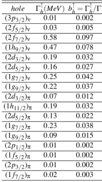
TABLE IV: Partial escape widths for one neutron and one proton direct decay fromISGDRin208Pbnucleus. The neutron and proton direct branching ratios are composed by (b↑)ν=0.32 and (b↑)π=

0.13 , respectively. The partial branching ratios are shown in the columnb↑_hfor each neutron and proton hole.

hole Γ↑_h(MeV) b↑_h=Γ↑_h/Γ

(3p_3/2)ν 0.01 0.002

(2f5/2)ν 0.03 0.005

(2f7/2)ν 0.58 0.097

(1h9/2)ν 0.47 0.078

(2d3/2)ν 0.19 0.032

(2d5/2)ν 0.16 0.027

(1g7/2)ν 0.25 0.042

(1g9/2)ν 0.22 0.037

(2d3/2)π 0.07 0.012

(1h11/2)π 0.19 0.032

(2d5/2)π 0.13 0.022

(1g_7/2)π 0.23 0.038

(1g9/2)π 0.09 0.015

(2p1/2)π 0.01 0.002

(1f5/2)π 0.01 0.002

(2p3/2)π 0.01 0.002

(1f7/2)π 0.02 0.003

TABLE V: The mean energy and total width (both in MeV) for ISGMR2 andISGQR2 in208Pb.

Mode This Work Ref.[48] Ref.[19] Exp. [26] ISGMR2 E 29.5 33.7 32.1 −

Γ 14 − − −

ISGQR2 E 31.5 − 30.5 26.9±0.7 Γ 6 − − 6.0±1.3

literature.

Concluding, we have presented a theoretical approach that improves the FKK method to include microscopic ingredi-ents, in order to calculate the spreading width of giant reso-nances. A important point is that the spreading width is cal-culated in connection with theRPAformalism. The residual interaction used inFKK approach is the same that was ad-justed inRPAcalculation.

IV. ACKNOWLEDGMENTS

This work was supported in part by Conselho Nacional de Desenvolvimento Cient´ıfico e Tecnol´ogico (CNPq), Brazil.

[1] G. Bertsch, P. F. Bortignon, and R. A. Broglia, Rev. Mod. Phys. 55,287 (1983).

[2] S. Kamerdzhiev, J. Speth, and G. Tertychny, Physics Reports 393, 1 (2004).

[3] S. Shlomo and G. Bertsch, Nucl. Phys. A243, 507 (1975). [4] K. F. Liu and N. Van Giai, Phys. Lett. B65, 23 (1976). [5] R. de Haro, S. Krewald, and J. Speth, Nucl. Phys. A388, 265

(1982).

[6] Ph. Chomaz, N. Van Giai, and S. Stringari, Phys. Lett. B189, 375 (1987).

[7] N. Van Giai, P. F. Bortignon, F. Zardi, and R. A. Broglia, Phys. Lett. B199, 155 (1987).

[8] A. F. R. de Toledo Piza, Rev. Bras. Fis.17, 195 (1987). [9] P. Curutchet, T. Vertse, and R. J. Liotta, Phys. Rev. C39, 1020

(1989).

[10] N. Teruya, A.F.R. de Toledo Piza, and H. Dias, Nuclear Physics A556, 157 (1993).

[11] C. Yannouleas, M. Dworzecka, and J. J. Griffin, Nuclear Physics A379, 256 (1982); ibid.397, 239 (1983).

[12] S. Drozdz, S. Nishizaki, J. Speth, and J. Wambach, Physics Re-ports197, 1 (1990).

[13] K. Takayanagi, K. Shimizu, and A. Arima, Nucl. Phys. A477, 205 (1988).

[14] J. S. Dehesa, S. Krewald, J. Speth, and A. Faessler, Phys. Rev. C15, 1858 (1977).

[15] S. Kamerdzhiev, G. Tertychny, J. Speth, and J. Wambach, Nucl. Phys. A577, 641 (1994); S. Kamerdzhiev, J. Speth, and G. Tertychny, ibid.624, 328 (1997).

[16] N. D. Dang, T. Suzuki, and A. Arima, Phys. Rev. C61, 064304 (2000); N. D. Dang, V. Kim Au, T. Suzuki, and A. Arima, ibid. 63, 044302 (2001).

[17] Denis Lacroix, Sakir Ayik, and Philippe Chomaz, Phys. Rev. C 63, 064305 (2001).

[18] G. Colo and P. F. Bortignon, Nucl. Phys. A696, 427 (2001). [19] M. L. Gorelik, I. V. Safonov, and M.H. Urin, Phys. Rev. C69,

054322 (2004).

[20] T. N. Leite and N. Teruya, Eur. Phys. J. A21, 369 (2004). [21] T. N. Leite, N. Teruya, and H. Dias, to be published in Int. J.

Mod. Phys. E.

[22] B. F. Davis, U. Garg, W. Reviol, M. N. Harakeh et. al., Phys. Rev. Lett.79, 609 (1997).

[23] H. L. Clark, Y. -W. Lui, D. H. Youngblood, K. Bachtr et. al. Nucl. Phys. A649, 57c (1999); H. L. Clark, Y. W. Lui, and D. H. Youngblood, Phys. Rev. C63, 031301(R) (2001).

[24] M. Uchida, H. Sakaguchi, M. Itoh, M. Yosoi et. al., Physics Letters B557, 12 (2003).

[25] M. Uchida, H. Sakaguchi, M. Itoh, M. Yosoi et. al., Phys. Rev. C69, 051301(R) (2004).

[26] M. Hunyadi, A. M. van den Berg, N. Blasi, C. Boumer et. al., Physics Letters B576, 253 (2003); Nucl. Phys. A731, 49 (2004).

[27] U. Garg, Nucl. Phys. A731, 3 (2004).

[28] H. Feshbach, A. Kerman and S. Koonin, Annals of Physics125, 429 (1980).

[29] T. N. Leite, and N. Teruya, Braz. J. Phys.35, 829 (2005). [30] R. Bonetti, M. B. Chadwick, P. E. Hodgson, B. V. Carlson, and

M. S. Hussein, Physics Reports202, 171 (1991). [31] P. Oblozinsky, Nucl. Phys. A453, 127 (1986).

[32] N. Teruya, A.F.R. de Toledo Piza, and H. Dias, Phys. Rev. C44, 537 (1991).

[33] T. N. Leite, N. Teruya, and H. Dias, Int. J. Mod. Phys. E11, 469 (2002).

[34] L. L. Salcedo, E. Oset, M. J. Vicente-Vacas, and C. Garcia-Recio, Nucl. Phys. A484, 557 (1988).

[36] S. Shlomo and A.I. Sanzhur, Phys. Rev. C65, 044310 (2002). [37] R. Bonetti and L. Colombo, Phys. Rev. C28, 980 (1983). [38] T. Kawano, Phys. Rev. C59,865 (1998).

[39] A. Veyssiere, H. Beil, R. Bergere, P. Carlos, and A. Lepretre, Nucl. Phys. A159, 561 (1970).

[40] N. Teruya, H. Dias and E. Wolynec, Phys. Rev. C37, 2121 (1988).

[41] B. Schwesinger and J. Wambach, Nucl. Phys. A 426, 253 (1984).

[42] S. Kamerdzhiev, J. Speth, G. Tertychny, and V. Tselyaev, Nucl. Phys. A555, 90 (1993).

[43] M. L. Gorelik, S. Shlomo, and M. H. Urin, Phys. Rev. C62,

044301 (2000).

[44] G. J. OKeefe, M. N. Thompson, Y. I. Assafiri, R. E. Pywell, and K. Shoda, Nucl. Phys. A649, 239 (1987).

[45] S. Strauch, Nucl. Phys. A649, 85c-92c (1999); S. Strauch, P. von Neumann-Cosel, C. Rangacharyulu, A. Richter et. al., Phys. Rev. Lett.85, 2913 (2000).

[46] S. Im and J. Meng, Phys. Rev. C61, 047302 (2000).

[47] I. Hamamoto, H. Sagawa, and X. Z. Zhang, Phys. Rev. C64, 024313 (2001).