Braz. J. Phys. vol.38 número3B

518 Brazilian Journal of Physics, vol. 38, no. 3B, September, 2008

Diffractive Higgs Boson Photoproduction in Peripheral Collisions

G. G. Silveira∗ and M. B. Gay Ducati†

Instituto de F´ısica, Universidade Federal do Rio Grande do Sul, Caixa Postal 15051, 91501-970 - Porto Alegre, RS, Brazil.

(Received on 4 June, 2008)

An alternative process is proposed for the diffractive Higgs boson production inspired in the Durham model, exploring it through the photon-proton interaction. In this sense, we estimate the production cross section of the Higgs boson, comparing some sets of parton distributions in the proton and confronting this results with those from other processes.

Keywords: Higgs boson; Diffractive process; Double Pomeron Exchange; Peripheral Collisions

1. INTRODUCTION

The detection of the Standard Model Higgs boson will be the main goal of the LHC. The lower bound on the Higgs mass was estimated experimentally being MH &114.4 GeV

with 95% confidence level [1]. A large set of possible dis-covery channels was studied (see [2, 3]), however the leading decay of the Higgs is expected to be observed as abb¯-pair in the mass rangeMH.140 GeV. A possible production of the

Higgs boson under study is the diffractive proccess by Double Pomeron Exchange (DPE) [4] inppcollisions.

We apply the same idea of DPE interaction, similar to the Durham group, with the interaction occurring in thet-channel of the subprocess photon-proton instead of the proton-proton system. For this proposal, the formalism of impact factor is used to describe the splitting of the photon into a color dipole and its interaction with the proton att=0.

2. PARTONIC PROCESS

The study of the diffractive production of the Higgs bo-son through theγ∗_{qis based on the kinematic variables used}

in the description of the Deeply Virtual Compton Scattering (DVCS), where the splitting photon interacts with the proton exchanging a gluon ladder [5]. The main feature present in this model of Higgs boson photoproduction is the interaction between the particles by DPE, providing the leading produc-tion vertex in the mass range where expect to observe ex-perimentally the Higgs boson. This kind of process is more studied in peripheral collisions, where the impact parameter is larger than the sum of the radius of the colliding particles (protons).

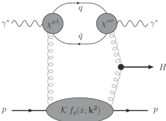
The Fig.1 shows the Feynman diagram for the subprocess of diffractive photoproduction. It represents four possibilities for the processγ∗_{q, all of them are obtained from the different}

coupling possibilities of the gluons to the fermions lines of the dipole.

The two-upper bubbles represent the effective vertices of the photon-gluon coupling which can be obtained through the

∗_{Electronic address:[email protected]} †_{Electronic address:[email protected]}

impact factor formalism [6]. The same formalism is used to explore the process with a non-zero momentum transfer with two gluons exchanged in thet-channel. The other bubble rep-resents the gluon density into the proton.

γ∗

χµλ

p p

H γ∗

χνσ

K_fg(x,k2₎

q

¯

q

FIG. 1: Feynman diagram representing the partonic process for diffractive Higgs production.

qµ _qµ

pµ _pµ

kµ

kµ

rµ

qµ

H

lµ

FIG. 2: Photoproduction subprocess of the Higgs boson.

The case studied here is based on the partonic subprocess

γ∗_q→γ∗_{+H+q illustrated in Fig.2. The central line cuts}

the diagram which represents the use of the Cutkosky rules to obtain the imaginary part of the scattering amplitude of the process through the expression

ImA=1

2

Z

G. G. Silveira and M. B. Gay Ducati 519

with

A

_Land

A

_{Rbeing the amplitudes on the left and right side} of the cut, respectively, andd(PS)3is the volume element of the three-body phase space. The scattering amplitude of the process is treated essentially as an imaginary quantity since the particle exchanged has the vacuum quantum numbers [7], so we can neglet the real one.

In the Dipole Model [8] the splitting of the photon into a quark-antiquark pair is treated by an wave function, where the product of this quantity with its complex conjugate represents the presence of the fermion loop.

Calculating the amplitude assigned in (1), the product of the left and right amplitudes results

A

_L

A

_{R= (4π)}3_α2

sα

Ã

∑

q

e2_q !_µ

εµε∗ν

k6 ¶_Vba

δσ

Nc

³ tbta´2

" Tµλσν

l4 +

Tλµσν l2_(k+l+q)2

#

4p_λpδ (2)

whereεµandε∗νare the polarization vectors of the initial and

final photons, respectively, andTi jkl are the traces from the dipole. The vectorlµis the four-momentum of the quark cir-culating in the fermion loop andpµ_{is the four-momentum of}

the colliding proton. There are four different diagrams to rep-resent the dipole in this process since the two gluons couple to its fermion lines. However, if both gluons couple to the up-per fermion line, it contributes equally as the couplings to the lower one. This equivalence also occur in the coupling to dis-tinct fermion lines. Thus, we need to take into account only one diagram with the gluons coupled to the same fermion line and other that they couple to different ones, and add a factor of 2 to include the other contributions.

The quantityVba

δσ represents the production vertexgg→H

which is known as [9] V_µab_ν =δab

µ gµν−

k2µk1ν

k1·k2 ¶

V, (3)

whereV_≈M2_Hαs/6πvbeing valid for the production of a

non-heavy Higgs boson (MH.200 GeV).

However, the value of traces involving a product of Dirac

γµ_{-matrices is obtained adopting an adjusted parametrization}

for the four-momenta present in the process. We adopt the Sudakov parametrization where the four-momenta are decom-posed under three base-vectors: two vectors of light-type pµ andq′µ_{, withq}′µ_=qµ_+xpµ_{, and a third vector lying in a plane}

perpendicular to the incident axis. The main kinematic vari-ables of interest are the center-of-mass energy s= (q+p)2 and the momentum fractionx=Q2/2(p_·q), with Q2 being the photon virtuality. The decomposition permits to write the four-momenta in the form

lµ = αℓq′µ+βℓpµ+lµ_⊥ (4a)

kµ = αkq′µ+βkpµ+kµ_⊥ (4b)

The polarization vectors do not depend on thet-variable, its sum being over transversal and longitudinal components expressed by the relations

εLµεLν∗ =

4Q2 s

pµpν

s (5a)

∑

εTµεTν∗ = −gµν+4

Q2 s

pµpν

s . (5b)

In order to reach our initial proposal, it is necessary to per-form the approximation on the photon virtuality taking the limitQ2

→0. This approximation is a realistic limit in the peripheral collisions context, in which the photon field around the hadrons is composed of real photons. Thus, we can sim-plify enormously obtaining the relation

(ImA)T =

10s 9

µ_M2

H

πv ¶

α3

sα

∑

q

e2_q µ

2CF

Nc

¶Z _dk2

k6 (6) We compute the cross section as a distribution in central-rapidity of the Higgs boson (yH=0), obtaining

dσ

dyHdp2H

=25α

4

sα2

23_81π3 µ_M2

H

Ncv

¶2Ã

∑

q

e2_q !2

·Z _α

sCF

π

dk2 k6

¸2

The main aspect obtained from this result is the sixth-order ~k-dependence compared to the result of Durham group, which had been obtained with a fourth-order dependence. This dif-ference appears due to the presence of the photon in the pro-cess which simplifies the result by the existence of only one parton distribution in the differential cross section.

3. PHOTON-PROTON COLLISIONS

A realistic case of photon-proton interaction in peripheral collisions is built if we substitute the contribution of the gluon-quark vertices by a partonic distribution into the proton to ex-press the coupling of the gluons to the proton, as illustrated by the lower blob of Fig.1.

However, the conditiont=0 is not sufficient to determine the gluon density function and it is necessary to assume a small value to the momentum fraction in this region of in-terest, asx_∼0.01, such that we can safely putt=0 [13].

Therefore, the follow replacement is made to describe the

γpinteraction

αsCF

π −→ fg(x,k

2_{) =K}

µ_∂[xg(x,k2_)]

∂ℓnk2 ¶

(7)

where fg(x,k2) is the non-diagonal gluon distribution

520 Brazilian Journal of Physics, vol. 38, no. 3B, September, 2008

Assuming a non-diagonal distribution it is possible to approx-imate this non-diagonality by a multiplicative factorKwhich possess a Gaussian shape [14]K= (1.2)exp(₋bp2

H/2), where

b=5.5 GeV−2 _{is the impact parameter. This factor can be} seen as a representation of the proton-Pomeron coupling.

Finally, the differential cross section has the form dσ

dy_H ¯ ¯ ¯ ¯

y_H=0

∼1_b

·Z _dk2

k6 fg(x,k 2₎

¸2

. (8)

An important feature considered by the Durham group is the suppression of the gluon emissions from the annihilation ver-tex, i.e., bremsstrahlung emissions [13]. The suppression probability for the emission of one gluon can be computed with the help of Sudakov form factors. For many emissions, this factor exponentiates and is taken into account by the in-troduction of an exponential factor to the gluon distribution.

A last important aspect involving diffractive processes is to compute the rapidity gaps present in the final state. These quantities are introduced in the model since the interaction be-tween the colliding particles occurs by means of an exchange of a particle with the vacuum quantum numbers, in this case, the Pomeron. Thus we consider a multiplicative factorS2_gap to include this physical aspect. Several approaches predict this quantity [15, 16], where the survival probability for Higgs production is estimated to be 3% for LHC (s=14 TeV) and 5% for Tevatron (s=1.96 TeV).

4. NUMERICAL RESULTS

Reaching our goal to build this model, we are able to calcu-late the differential cross section for the Higgs boson diffrac-tive production through theγpinteraction. Avoiding infrared divergencies we made a cut in the integration on the gluon transverse momentum [10].

60 80 100 120 140 160 180 200

MH (GeV) 0

0,1 0,2 0,3 0,4 0,5

d

σ

/dy

H

(y

H

= 0) (fb)

Forshaw Fotoprodução LHC :: E = 14 TeV

MRST2001lo Q20 = 1.25 GeV

2

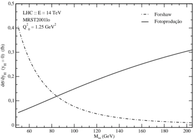
FIG. 3: Differential cross sectiondσ/dyH(yH=0)for LHC energy.

The first step is to compare the results obtained with this model with those obtained before for the production in di-rectpp collisions. For this proposal we compare our results with the results of the Durham group implemented by For-shaw [10]. The prediction for the differential cross section in

central-rapidity for LHC is calculated using the parametriza-tion MRST2001 in leading order approximaparametriza-tion for the gluon distribution function taking an initial cut ofk20=1.25 GeV2. The result is expressed in Fig.3 where the differential cross section is fitted in function of the Higgs boson mass. There-fore the behavior of the photoproduction results is expected to not fit like the results of directppcollisions due to the pres-ence of only one parton distribution in theγpapproach.

200 400 600 800 1000 1200 1400 MH (GeV)

0 0,01 0,02 0,03 0,04

d

σ

/dy

H

(y

H

= 0) (fb)

MRST2001lo MRST2004nlo CTEQ6mE ALEKHIN02lo Tevatron :: E = 1.96 TeV

Q20 = 1.00 GeV 2

200 400 600 800 1000 1200 1400 MH (GeV)

0 0,25 0,5 0,75 1 1,25 1,5

d

σ

/dy

H

(y

H

= 0) (fb)

MRST2001lo MRST2004nlo CTEQ6mE ALEKHIN02lo LHC :: E = 14 TeV

Q20 = 1.00 GeV 2

FIG. 4: Differential cross sectiondσ/dyH(yH =0)for energies of

Tevatron and LHC

Extending these numerical analyses we predict the dif-ferential cross section adopting some distributions functions for the gluon content into the proton, which is shown in Fig. 4. The non-diagonality of the distributions was ap-proximate by a multiplicative factor which permit us to ac-count the usual diagonal distributions. All these distributions were evolved from an initial momentumk2₀=1 GeV2, value adopted to be an average between the initial cuts assumed by each parametrization. As an evidence we can see a gap in the results to LO and NLO distributions in this range of energy.

G. G. Silveira and M. B. Gay Ducati 521

5000 10000 15000 20000

E (GeV) 0

0,001 0,002 0,003 0,004 0,005

d

σ

/dy

H

(y

H

= 0) (fb)

M_H = 120 GeV M_H = 140 GeV M_H = 180 GeV MRST2001lo

Q2₀ = 1.00 GeV2

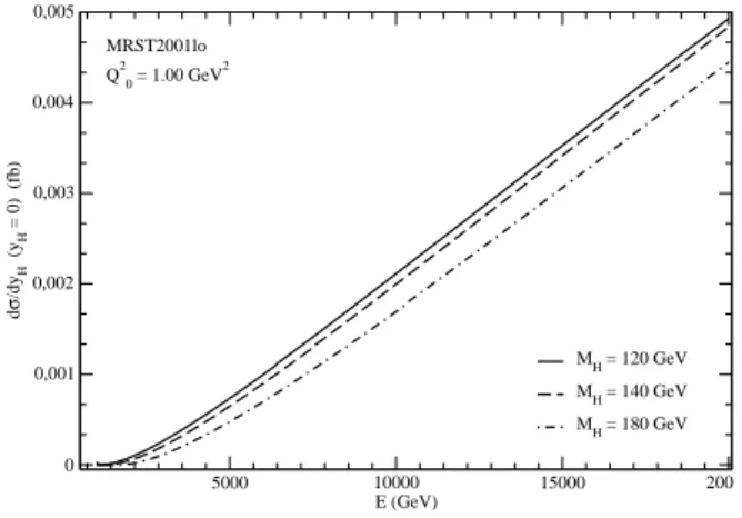
FIG. 5: Differential cross sectiondσ/dyH(yH=0)varying the Higgs

mass.

5000 10000 15000 20000

E (GeV) 0

0,001 0,002 0,003 0,004 0,005 0,006

d

σ

/dy

H

(y

H

= 0) (fb)

MRST2001lo MRST2004nlo CTEQ6mE ALEKHIN02lo M_H = 140 GeV

Q2₀ = 1.00 GeV2

FIG. 6: Differential cross sectiondσ/dyH(yH=0)for different PDF

in the process.

shape due to its quartic dependence on the Higgs mass. The Sudakov form factors acts to increase the results stating a linear shapes for higher energies. This dependence is anal-ysed with the distribution functions used before presenting the same linear behavior for higher energies, showed in Fig.6. An important aspect observed in this second analysis is the same difference between LO and NLO distribution functions ob-served before.

5. CONCLUSIONS

The numerical results obtained in this approach demanded a more complex calculation since it was computed the dipole contribution in the Higgs boson production by DPE. As a re-ward we could obtain a simple result to the event rate, however from a more complex physical process than those studied by the Durham group. Performing the phenomenological anal-yses, the results show an event rate of the order of 1 fb, in accord to the predictions from other diffractive processes for Higgs production. We expect an agreement to the previous results of the Durham group when a more complete study be performed with the introduction of a photon distribution into the proton, and to effectively compute the Higgs production in peripheral hadron-hadron collisions.

Acknowledgements

This work is partially supported by CNPq (G.G.S. and M.B.G.D.).

[1] R. Barate et al, Phys. Lett. B565, 61 (2003).

[2] M. Carena, H. Haber, Prog. Part. Nucl. Phys.50, 1 (2003). [3] T. Hahn et al, arXiv:hep-ph/0607308.

[4] A. Bialas, P.V. Landshoff, Phys. Lett. B256, 540 (1991). [5] L. Frankfurt et al, Phys. Rev. D58, 114001 (1998).

[6] J. R. Forshaw, N. G. Evanson, Phys. Rev. D60, 034016 (1999). [7] L. Foldy, R. F. Peierls, Phys. Rev.130, 1585 (1963).

[8] A. H. Mueller, Nucl. Phys. B415, 373 (1994), Phys. Rev. B 437, 107 (1995).

[9] B. A. Kniehl, Phys. Rep.240, 211 (1994). [10] J. R. Forshaw, arXiv:hep-ph/0508274.

[11] V. A. Khoze, A. D. Martin, and M. G. Ryskin, Eur. Phys. J. C

14, 525 (2000).

[12] K. J. Golec-Biernat, A. D. Martin, Phys. Rev. D59, 014029 (1998).

[13] V. A. Khoze, A. D. Martin, and M. G. Ryskin, Phys. Lett. B 401, 330 (1997).

[14] A. G. Shuvaev et al, Phys. Rev. D60, 014015 (1999).

[15] V. A. Khoze, A. D. Martin, and M. G. Ryskin, Eur. Phys. J. C 18, 167 (2000).