www.ann-geophys.net/26/1935/2008/ © European Geosciences Union 2008
Annales
Geophysicae
Verification of a coupled atmosphere-ocean model using satellite
observations over the Adriatic Sea
V. Djurdjevic and B. Rajkovic
Institute of Meteorology, Faculty of Physics, Belgrade University, Belgrade, Serbia
Received: 24 July 2007 – Revised: 6 June 2008 – Accepted: 12 June 2008 – Published: 16 July 2008
Abstract. Verification of the EBU-POM regional atmosphere-ocean coupled model (RAOCM) was carried out using satellite observations of SST and surface winds over the Adriatic Sea. The atmospheric component has a horizon-tal resolution of 0.125 degree (approximately 10 km) and 32 vertical levels, while the ocean component has a horizontal resolution of approximately 4 km with 21 sigma vertical lev-els.
Verification of the forecasted SST was performed for 15 forecasts during 2006, each of them seven days long. These forecasts coincide with the operating cycle of the Adri-atic Regional Model (AREG), which provided the initial fields and boundary conditions for the ocean component of EBU-POM. Two sources of data were used for the initial and boundary conditions of the atmosphere: primary data were obtained from the European Center for Medium-Range Weather Forecasting (ECMWF), while data from National Centers for Environmental Prediction (NCEP) were used to test the sensitivity to boundary conditions.
Forecast skill was expressed in terms of BIAS and root mean square error (RMSE). During most the of verification period, the model had a negative BIAS of approximately −0.3◦, while RMSE varied between 1.1◦and 1.2◦. Interest-ingly, these errors did not increase over time, which means that the forecast skill did not decline during the integrations. The 10-m wind verification was conducted for one period of 17 days in February 2007, during a strong bora episode, for which satellite estimates of surface winds were available. During the same period, SST measurements were conducted twice a day, which enabled us to verify diurnal variations of SST simulated by the RAOCM model. Since ECMWF’s deterministic forecasts do not cover such a long period, we decided to use the ECMWF analysis, i.e. we ran the model in hindcast mode. The winds simulated in this analysis were
Correspondence to:V. Djurdjevic ([email protected])
weaker than the satellite estimates, with a mean BIAS of −0.8 m/s.
Keywords. Meteorology and atmospheric dynamics (Mesoscale meteorology) – Oceanography: general (Ocean prediction) – Oceanography: physical (Air-sea interactions)
1 Introduction
Ocean forecasts are needed in areas such as transportation, exploitation of marine and bottom regions, environmental is-sues, and security issues. Compared with weather (atmo-spheric) forecasting, the forecasting of the oceans or seas is a relatively new idea. It has only recently become possible due to increased knowledge about the state of the oceans and seas. Previously, global and local climatological methods of-fered only relatively low resolution. Because of advances in what can be accurately measured using classical and mod-ern devices, and because of the use of remote sensing and measurements of SST and sea surface elevation, we are able, at least in some world regions, to obtain a three-dimensional snapshot of ocean conditions accurate enough for forecasting purposes.
The two biggest challenges to forecasting are knowledge of the initial fields, as mentioned above, and reliable forc-ing data, which must be supplied from an atmospheric fore-cast model. In contrast to the relatively fast time scale of atmospheric change, time scales for ocean changes are much longer, so a short-range forecast of 7–10 days for the ocean is at the edge of reliability of atmospheric forecasts. In ad-dition to their longer time scales, oceans, and in particular shallower seas, develop structures with much shorter spatial scales. Thus, we need relatively high-resolution atmospheric forcing.
analysed the Adriatic response to wind forcing by creating a modified bora and siroco climatology, and they were able to reproduce the general features of the sea. During bora winds, the response was quite complex, developing several lows and highs in agreement with the wind stress curl field. In the case of siroco, the currents produced were controlled by the bottom slope and wind stress curl. In some cases, siroco may cause the reversal of currents along the Adri-atic western coast. Artegiani et al. (1997) defined the open ocean seasonal climatology of the basin based on a compre-hensive historical hydrographic dataset for the overall Adri-atic Sea basin. They also defined the regional climatological seasons by computing the average monthly values of heat fluxes and heat storage using a variety of atmospheric data sets. Using these data sets, they examined heat exchange and storage. Enger and Grisogono (1998), in an idealized 2-D study of bora winds, evaluated the influence of higher or lower uniform ocean temperature on the bora wind, and the influence of the SST structure on its extension over the Adri-atic. Beg Paklar et al. (2001) examined the response of the Adriatic shelf waters and the Po river plume to a bora wind episode using a combination of the Princeton Ocean Model (POM) and the NCAR Mesoscale Model (MM5). Using a bulk method, atmospheric forcing was calculated from the winds, air temperatures, and humidities obtained by MM5, with spatial resolution of 9 km and temporal resolution of 1 h. They concluded that high horizontal resolution in the nu-merical experiments is important for resolving the variability of the bora wind field along the shore and to correctly sim-ulate the narrow filament observed in AVHRR images. Za-vatarelli et al. (2002) analysed two different forcings based on ECMWF products, and found that the circulation shows large seasonal variability, with a largely barotropic state dur-ing winter and a baroclinic structure durdur-ing summer. They also found that amplitudes may be affected by the strength of the wind-forcing field.
In 2002 and 2003, intensive, multidisciplinary studies of the northern and central Adriatic were conducted (Lee et al., 2005; Pasaric et al., 2006; Pullen et al., 2007; Jef-fries and Lee, 2007; Dorman et al., 2006; Peters et al., 2007). This research involved significant empirical and modelling studies. The DOLCEVITA program (The Dy-namics of Localized Currents and Eddy Variability in the Adriatic) investigated the mesoscale and sub-mesoscale re-sponse to strong atmosphere and river forcing within the context of large-circulation studies. This projecthowed that with extremely high-resolution atmospheric forcing, includ-ing non-hydrostatic regimes, ocean models can form notice-able, albeit short-lived, surface current structures. In addi-tion to DOLCEVITA, several other field programs were car-ried out in 2002–2003, such as the Mesoscale Alpine Pro-gram (MAP, 1999), the European Margin Strata Formation EUROSTRATAFORM), and the Adriatic Circulation, West Istria, and East Adriatic Coastal Experiments (ACE, WISE, EACE).
Pullen et al. (2003), in high-resolution studies of the Adri-atic using the Navy Coastal Ocean Model (NCOM; 2-km resolution) forced by COAMPS (4- and 36-km resolution), were able to produce realistic fine-scale bora features with an enhanced-resolution atmospheric model. The superior at-mospheric forecasts produced by the 4-km nested grid com-pared to the 36-km nested grid also improved the ability of the ocean model to generate wind-forced currents when evaluated against Acoustic Doppler Current Profiler (ADCP) observations. Mantziafou and Lascaratos (2004) analysed general circulation and deep-water formation (DWF) pro-cesses in the Adriatic basin using climatological forcing us-ing ECMWF Reanalysis data (1◦×1◦) from 1979–1994. The
model reproduced the main basin features of the general cir-culation, as well as the water mass distributions and their seasonal variability. They showed that the DWF rates and their mass characteristics in a given year depend not only on the atmospheric conditions prevailing for that year, but on conditions prevailing during the previous year as well, thus leading to the concept of a “memory” of the basin. Signell et al. (2005) assessed the wind quality in oceanographic mod-elling by indirectly comparing simulated waves using the SWAN model to wave measurements at the ISMAR oceano-graphic tower in Venice. In that study, the authors analysed forcing in three different models of increasing horizontal res-olution:. ECMWF; LAMBO, LAMI; and COAMPS. They were able to demonstrate that increased horizontal resolution increases the quality of the forcing.
Mediterranean; these systems differed in both their spatial but and temporal scales.
Similarly to their work in 2003 (Pullen et al., 2003), Pullen et al. (2007) used the semi-coupled NCOM model and the coupled COAMPS model, both with relatively high resolu-tion (2–4 km for the ocean and atmosphere, respectively) to investigate situations with both strong and weak winds. They assessed their results using remote and in situ measurements over water, as well as coastal wind observations. These stud-ies also analysed coupled and semi-coupled configurations. They demonstrated that the coupled model performed better. Several of these papers showed clearly that relatively high-resolution atmospheric forcing is required to resolve or re-produce mesoscale features documented in extensive field in-vestigations. In most of these studies, the modellers created fluxes from diagnostically computed, 2-m temperatures and 10-m winds using the corresponding atmospheric model, var-ious bulk models, or some other approach. Although slightly inconsistent, this approach does succeed in taking into ac-count high-resolution features in the developed SST. This is important because ocean-atmosphere temperature gradients play a very important role in energy exchange.
In addition to atmospheric forcing, fresh water inflow plays an important role due to the relatively small size of the Adriatic. At present, global models are the main sources of forcing fields for periods of 5–10 days. They all include some degree of interaction with the ocean surface, either by being coupled to an ocean model of more or less complexity, or by specifying SST, usually through some type of clima-tology. Limited-area models are another possible source of atmospheric forcing, though these rely on the initial fields and boundary conditions of global models. Due to a gen-eral increase in the quality of these global and limited-area models, the number of operational or semi-operational ocean forecasts is rapidly increasing. A two-step approach that uses a global and then a limited-area model solves the problem of the need for high-resolution forcing. Similarly to the case of an atmospheric model, the Local Ocean model relies on a global (basin) scale model for initial and boundary condi-tions. Such forecasts are produced at several centres. For the Mediterranean Sea, the operational forecasting system MF-STEP (Pinardi et al., 2003) covers the whole basin and is run at INGV in Bologna. Using these forecasts as a starting point, regional or coastal models are run in several regions of the Mediterranean Sea. The regional or coastal models usually have higher spatial resolution. They are forced either with the same forcing used in the MFSTEP forecasts, or with different atmospheric forcing. This hierarchy of model do-mains solves or simplifies the problem of the boundary con-ditions, which is the third-biggest problem in ocean forecast-ing.
From October 2001 to November 2006, two large projects were devoted to beginning operational forecasts for the Adriatic Sea: the Adriatic Sea Integrated Coastal Ar-eas and River Basin Management System Project
(ADRI-COSM), and its extension (ADRICOSM-EXT) (Zavatarelli and Pinardi, 2003; Manzella et al., 2003). This forecasting system, operating under the name AREG, has been run once a week since April 2003. The Institute of Meteorology at the Faculty of Physics of Belgrade University focused on pro-ducing the atmospheric forcing. For this purpose, a coupled, limited-area, atmospheric-ocean model was created with the aim of increasing the quality and length of the forecast. The atmospheric component is the Eta Belgrade University model (EBU), NCEP’s operational model at the time, and the ocean component is the Princeton Ocean Model (POM).
Ocean simulations or forecasts can be verified in several ways. The most direct and most accurate way is through in situ measurements. Nevertheless, even where such mea-surements are available, their spatial coverage is usually lim-ited, and therefore some kind of spatial interpolation must be used. The other two alternatives are remote sensing of SST or the indirect approach of coupling a wave model to an ocean model and verifying the results (Signell et al., 2005). The question of forcing, i.e., measuring the fluxes, is far more complicated. In principle, fluxes can be measured in situ, but due to their high spatial and temporal variation, we require even denser networks than for mean fields in order to repre-sent them properly.
The other possibility is remote measurements of 10-m winds and STT, which we compare with the 10-m winds and SST forecast by an atmospheric model. A limitation of this method is time sampling, since successive satellite passes oc-cur only every 12 or 24 h, and the spatial resolution is limited to approximately 25 km. At present, in situ measurements remain superior to remote measurements, which also can be limited by precipitation or clouds in the area of interest. Nev-ertheless, remote sensing of ocean fields does present three important advantages over in situ measurements: (1) a much larger area can be covered in a way that is uniform both through time and space, and at a higher sampling frequency than in possible with other approaches; (2) the spatial res-olution is much higher; and (3) they can easily be incorpo-rated into an operational system. Within both ADRICOSM projects, the CNR-ISAC (Rome) sought to supply the project community with both SST and 10-m wind measurements. We have conducted our verification using those data.
2 The model
The model is a fully coupled atmosphere-ocean model with exchanges of fluxes and SST performed at every atmospheric physics time step, with atmospheric resolution of 0.125◦,
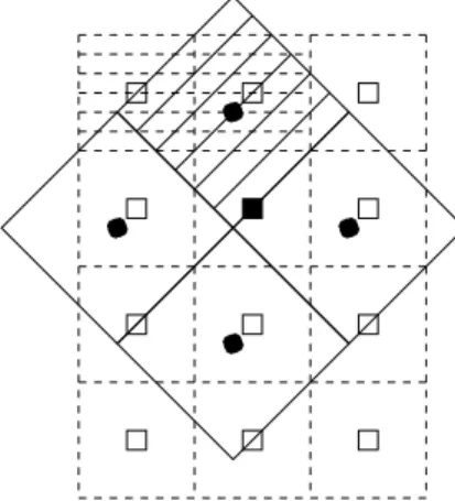
Fig. 1. Overlap of the atmosphere and ocean model domains. The atmosphere domain is in gray, while the ocean domain is the black rectangle at the centre of the picture.
and SST. Exchanged fluxes are calculated using the atmo-spheric component and used directly, without any additional parameterization.
2.1 The atmospheric component
The atmospheric component is a limited-area forecast model defined on the E-grid according to the nomenclature of Arakawa and Wininghoff (Winninghoff, 1968; Arakawa and Lamb, 1977) and with eta vertical coordinate (Mesinger et al., 1988). Its dynamic core has an efficient time-stepping, with a short time-step for the forward-backward gravity wave scheme modified so as to address the E-grid’s lattice separa-tion problem (Mesinger, 1974; Janjic, 1979), a longer time step for its conservative advection schemes (Janjic, 1984), and a still longer time step for the physics terms. The physics package consists of a surface scheme (Mahrt et al., 1988), a radiation scheme (Fels and Schwarzkopf, 1975), a turbu-lence closure sub-model (Mellor and Yamada, 1974; Mellor and Yamada, 1982; Janjic, 1990), a viscous sub-layer (Jan-jic, 1996) and a convection parameterization (Betts, 1986; Betts and Miller, 1986; Janjic, 1990). The centre of the at-mospheric model is at 16◦E, 42.5◦N and the horizontal
res-olution is 0.125◦. In the vertical direction, the model has 32
levels, with the first level at 20 m and the top at 10 mb.
10-Jan 11-Jan 12-Jan 13-Jan 14-Jan 15-Jan 16-Jan 17-Jan 18-Jan 19-Jan 20-Jan 21-Jan 22-Jan 23-Jan 24-Jan 25-Jan 26-Jan 27-Jan 28-Jan 29-Jan 30-Jan 31-Jan 01-Feb 02-Feb 03-Feb 04-Feb 05-Feb 06-Feb 07-Feb 08-Feb 09-Feb 10-Feb 11-Feb 12-Feb 13-Feb 14-Feb 15-Feb 16-Feb 17-Feb 18-Feb 19-Feb 20-Feb 21-Feb 22-Feb 23-Feb 24-Feb 25-Feb 26-Feb 27-Feb
date
-1 -0.8 -0.6 -0.4 -0.2 0 0.2 0.4 0.6 0.8 1 1.2 1.4 1.6
°
C
BIAS and RMSE (model vs. satelite observation)
-1 -0.8 -0.6 -0.4 -0.2 0 0.2 0.4 0.6 0.8 1 1.2 1.4 1.6
°
C
rmse
bias
BIAS and RMSE (model vs. satelite observation)
Fig. 3.Daily values of area-averaged BIAS and RMSE for the period of 10 January–27 February 2006.
2.2 The ocean component
POM is a three-dimensional, primitive equation, numerical model (Blumberg and Mellor, 1987; Mellor, 2002). Its hor-izontal grid uses curvilinear orthogonal coordinates on a C-grid (Arakawa and Wininghoff nomenclature), and its ver-tical coordinate is a sigma coordinate. The model has effi-cient time differencing, which is explicit in horizontal and implicit in vertical. It has a free surface, complete thermo-dynamics, and, second-order turbulence closure. Advection schemes use the finite volume approach, which is particularly suitable when using curvilinear orthogonal coordinates. Fig-ure 1 shows both atmospheric and oceanic domains. Since the ocean component was initialized using AREG fields, we adopted the same geometry as in AREG in order to avoid horizontal and vertical interpolation. The model’s grid is a regular lat-lon grid covering the region 39.0–46.0◦N, 12.0–
20.0◦E with horizontal resolution of 4 km and with 21
verti-cal levels.
2.3 The coupler
Due to the very different geometries of the two model com-ponents, special care was taken in coupling them together. In Fig. 2 we present a schematic representation of the over-lap of these two grids in the models. In addition to different positions of the corresponding points, there is also a differ-ence in the horizontal resolution in the two sub-models. The atmospheric component has a resolution roughly four times coarser than the oceanic one. That led to different land-sea masks, since both the atmosphere and ocean “saw” different distributions of sea and land. Thus, the same point could be seen as a land point by the atmospheric component and as an ocean point by the ocean sub-model. As a result, because of large differences in heat and momentum fluxes over land and sea, the energy and momentum exchange between the sea and the atmosphere would be wrong.
0 500 1000 1500 2000 2500 3000 3500 4000 4500 5000 5500 6000 6500 7000 7500 8000 8500 9000
number of points
10-Jan 11-Jan 12-Jan 13-Jan 14-Jan 15-Jan 16-Jan 17-Jan 18-Jan 19-Jan 20-Jan 21-Jan 22-Jan 23-Jan 24-Jan 25-Jan 26-Jan 27-Jan 28-Jan 29-Jan 30-Jan 31-Jan 01-Feb 02-Feb 03-Feb 04-Feb 05-Feb 06-Feb 07-Feb 08-Feb 09-Feb 10-Feb 11-Feb 12-Feb 13-Feb 14-Feb 15-Feb 16-Feb 17-Feb 18-Feb 19-Feb 20-Feb 21-Feb 22-Feb 23-Feb 24-Feb 25-Feb 26-Feb 27-Feb
date
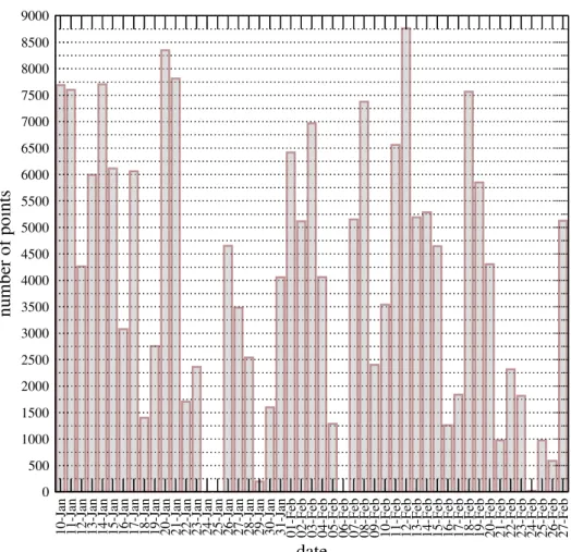
Fig. 4.Number of model grid points with satellite observations availabe.
points are computed in the following way: first, we com-pute average flux, with averaging carried out for all points in the first group. This serves as the first guess value. This value is improved by applying a Laplacian operator over the points belonging only to the second group. Fluxes for the first group are not changed by this procedure. As previously noted, the exchange of fluxes and SST is conducted every time that physics is done in the atmospheric model. At the end of this step, the surface fluxes are diagnosed and taken by the “coupler”. The fluxes in question are the following: the momentum flux; two heat fluxes, latent and sensible; and two radiative fluxes, short- and long-wave. The latent heat flux is the sink for fresh water. The coupler interpolates values hor-izontally onto the ocean grid. Interpolated fluxes force the ocean over several ocean time steps with total length equal to the atmospheric physics time step. The ocean surface then has an updated temperature that is read by the “coupler”. For-mation of SST on the atmospheric grid is done by averaging over four ocean points that correspond to one atmospheric point, except near coasts where three or even two points may be used.
2.4 The model setup
Fig. 5.Mean SST BIAS over the Adriatic area for four periods of seven days each: 10–16, 17–23, 24–30 January, and 31 January–6 February.
3 Remote sensing of SST and surface winds
Satellite oceanography is important for operational appli-cations because satellite-based sensors can collect
Fig. 6.Mean SST BIAS for three, seven-day periods 7–13, 14–20, 21–27 February and the entire period of 10 January–27 February over the Adriatic area.
partner modelling centres with remotely sensed ocean colour, sea surface temperature (SST) and, for a selected period, surface wind. Data are processed, mapped, and binned for
03-Apr 04-Apr 05-Apr 06-Apr 07-Apr 08-Apr 09-Apr 10-Apr 11-Apr 12-Apr 13-Apr 14-Apr 15-Apr 16-Apr 17-Apr 18-Apr date -1 -0.8 -0.6 -0.4 -0.2 0 0.2 0.4 0.6 0.8 1 1.2 1.4 1.6 ° C bias rmse
22-May 23-May 24-May 25-May 26-May 27-May 28-May 29-May 30-May 31-May 01-Jun 02-Jun 03-Jun 04-Jun 05-Jun 06-Jun date -1 -0.8 -0.6 -0.4 -0.2 0 0.2 0.4 0.6 0.8 1 1.2 1.4 1.6 1.8 2 2.2 2.4 ° C bias rmse
12-Jun 13-Jun 14-Jun 15-Jun 16-Jun 17-Jun 18-Jun 19-Jun 20-Jun 21-Jun 22-Jun 23-Jun 24-Jun 25-Jun 26-Jun 27-Jun date -1 -0.8 -0.6 -0.4 -0.2 0 0.2 0.4 0.6 0.8 1 1.2 1.4 1.6 1.8 2 2.2 2.4 2.6 2.8 ° C bias rmse
26-Jun 27-Jun 28-Jun 29-Jun 30-Jun 01-Jul 02-Jul 03-Jul 04-Jul 05-Jul 06-Jul 07-Jul 08-Jul 09-Jul 10-Jul 11-Jul date -1 -0.8 -0.6 -0.4 -0.2 0 0.2 0.4 0.6 0.8 1 1.2 1.4 1.6 1.8 2 ° C bias rmse
Fig. 7.BIAS and RMSE scores for eight forecasting periods, 3–18 April, 22 May–6 June, 12–26 June and 27 June–11 July, grouped in sets of two.
have permitted the building and optimization of a system suitable for meeting the increasing demand for near-real-time ocean colour and SST. Real-time images of SeaWiFS chloro-phyll concentration, clouds/case I/case II, water flags, and true colour images, are obtained by processing the satellite passes using ancillary climatological data. These images are provided daily through an ad hoc automatic system that pro-cesses the raw satellite data and makes them available on the
Web within an hour of satellite acquisition. NOAA/AVHRR data are also acquired by the GOS ground station in Rome and managed by the FDS from the reception stage through to distribution. Daily SST maps of the Adriatic Sea are binned over the AREG model grid at 1/16◦resolution. Derivation of
7 8 9 10 11 12 13 14 15 16 temperature (°C) observation model
10-Feb 11-Feb 12-Feb 13-Feb 14-Feb 15-Feb 16-Feb 17-Feb 18-Feb 19-Feb 20-Feb 21-Feb 22-Feb 23-Feb 24-Feb 25-Feb 26-Feb 27-Feb 28-Feb date -0.6 -0.4 -0.2 0 0.2 0.4 0.6 0.8 bias mean bias=0.042
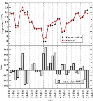
Fig. 8. Time series of diurnal variations of averaged SST (upper panel) and BIAS (lower panel) between model (red) and observa-tions (black). Note that the observation areas are different for each date. This is a result of changes in satellite coverage from day to night. See the next figure for explanation.
Geophysical conversion is the transformation from sensor counts to single-channel radiance and multi-channel derived SST. The Pathfinder algorithm (Walton et al., 1998; Kil-patrick et al., 2001) has been identified as the algorithm pro-viding the most accurate SST’s based on comparison with independent observations (within 0.2◦C). Moreover, it was
tested on observations from the Mediterranean Sea inde-pendent of the observations used to develop the algorithm, and it gave results equivalent to those of the global data set (D’Ortenzio and Marullo, 20000).
Remapping is the specification and application of a par-ticular projection on which the image can be mapped. The specified mathematical transform is applied to a navigated image consisting of scaled geophysical data. Remapped data are specified only by the projection, the latitudinal and lon-gitudinal centre of the image, and the output pixel size. The projection applied to the images is equi-rectangular, and it is the same projection as implemented in SeaWiFS to super-impose different products. The dimensions of the remapped images in the Adriatic Sea are 512×600, ranging from lati-tude 39.0–46.0 N and longilati-tude 12.0–20.0 E.
Declouding is the identification of cloud-contaminated pixels in SST imagery. The Pathfinder SST procedures con-struct quality control fields based on spatial uniformity tests and deviations from the Optimally Interpolated REYNOLDS fields (1◦resolution, weekly average global SST), published
weekly by NOAA. Low-quality pixels are defined as
cloud-contaminated. However, this automated declouding pro-cedure can erroneously identify clouds in areas of strong oceanic cloud fronts due to the coarse resolution of the REYNOLDS fields. Improvements to the declouding pro-cedure are needed in the Adriatic Sea, where coastal fronts are strong. For more details, see Sciara et al. (2006).
4 Results
4.1 Verification of SST
All forecasts cover the period of 10 January to 17 July 2006. Results are presented in terms of BIAS and RMSE scores for the area-averaged SST (see Appendix for definitions). In Fig. 3, we present the verification of SST from 10 January to 27 February. It is important to note that although the figure shows results in a continuous fashion, the results comprise seven consecutive forecasts. The gap around 27 January is because satellite measurements were unavailable for that pe-riod. Figure 4 shows the frequency of the satellite observa-tions during the same period. The mean value of RMSE was between 1.1◦ and 1.2◦, while BIAS was between 1.2◦ and
−1.1◦, with negative values during most of the period. The
mean BIAS was approximately−0.3◦, which is very close to
the observational error of 0.2◦.
Importantly, the RMSE within each of the forecasts does not increase with time. In many cases, the error is largest at the beginning of the forecast period and it decreases as time goes on. Comparing each forecast score with number of grid points for which satellite observations were available, (19 January; 5, 7, 17, 21, and 24 February) shows that all large BIAS/RMSE values occur when the number of obser-vations is small. A more complete picture of the differences between model and satellite SST is presented in Figs. 5 and 6, where we show horizontal variations of SST BIAS over the Adriatic area for periods of 10 January–6 February and 7–27 February, respectively. We can see that over most of the area, BIAS is small (see light blue and light yellow colours). Near the coast, BIAS has larger absolute values and occurs nearly equally as negative and positive numbers. This phenomenon is a well-known problem when verifying SST from satellites in coastal areas with shallow waters. The last panel shows the mean BIAS for the entire seven-week period, from which we can conclude that BIAS exhibits the same behaviour. In Fig. 7, we present the BIAS and RMSE for the remaining forecasts. Scores exhibit similar behaviour, except for a sin-gle forecast from 20 to 27 June, when RMSE starts with a value of 2.7◦. Even in that case, however, the RMSE
de-creases towards the end of the forecast.
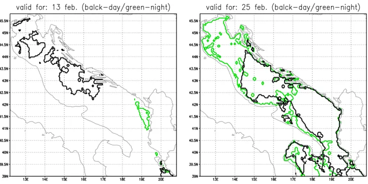
Fig. 9. The left panel shows an example of very small overlaps in satellite coverage from day to night. The data come from 13 February 2006. The green line denotes the night satellite pass, while the black line denotes the day satellite pass. Note that the two areas overlap only at the south entrance of the Adriatic and only very close to the Albanian coast. The right panel shows satellite coverage for 25 February. Note that in this case, the day and night coverage overlaps over an extensive portion of the Adriatic Sea.
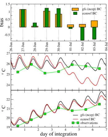
check how the choice of data set can affect the resulting fore-casts, we performed the same forecasts with the same model set-up but using NCEP fields. Nearly all NCEP-derived fore-casts were quite close to the ECMWF-derived forefore-casts, ex-cept for the one shown in Fig. 10. The top panel shows BIAS for the 26 June forecast, showing the closeness between the two forecasts for the first four days. After the fourth day, the ECMWF-derived forecast deteriorates, while the BIAS for the NCEP-based forecast remains small. The middle panel shows the variation in SST over time, with the SST aver-aged over the entire Adriatic region in both forecasts. The ECMWF-based forecast is in red, the NCEP-based forecast is in black, and observations are in green. As with the BIAS score, we see that the two forecasts agree well for the first four days, after which the ECMWF-based one begins to de-viate from the observations. Note that the SST was averaged over the whole Adriatic, whereas the observation area was smaller. Based on an examination of synoptic charts, the rea-son for this difference was that the ECMWF forecast did not capture the intensity and position of the front that was cross-ing the Adriatic durcross-ing the period under study. Finally, the bottom panel shows a typical case where the two forecasts differ only slightly.
4.3 Verification of the diurnal variation in SST
Verification of the diurnal variation of SST is possible us-ing data from two successive satellite passes. Results from
the period from 10–27 February are presented in Fig. 8, with area-averaged SST shown in the upper panel and BIAS scores in the lower panel. The fields are for midnight and noon, local time, for a particular date; observations are marked with squares and forecasts are marked with circles. Dotted lines indicate midnight for each day. It should be noted that large variations in averaged SST, from one pair to another, are a result of differences in the size and position of verification areas, which depended on the cloud-free area. Possible differences in the area coverage are shown in Fig. 9, with the two panels corresponding to two different days, 13 and 25 February. The green line is the border of the cover-age during the night, and the black line is the border of the coverage during the day. Therefore, for 13 February, the area covered by both night and day passes is very small and very close to the shoreline, while for 25 February, joint coverage was quite large. The corresponding differences between ob-served and forecasted SST are large for the first date and very small for the second one.
26-Jun 27-Jun 28-Jun 29-Jun 30-Jun 01-Jul 02-Jul 03-Jul 04-Jul -0.5 0 0.5 1 1.5
bias
gfs (ncep) BC ecmwf BC 24 25 26 27 ° C
0 1 2 3 4 5 6 7
day of integration
19 20 21 22 ° C
gfs (ncep) BC ecmwf BC observations
Fig. 10. The top panel shows BIAS scores for two different ini-tial and boundary conditions. NCEP data are shown in orange, ECMWF data are shown in green. The period of integration was 26 June–4 July, 2006. The middle panel shows time series of area-averaged SST over the whole Adriatic from both forecasts for the same period as in the previous figure; ECMWF is shown in red, NCEP in black, and observations in green. The bottom panel shows a time series of area-averaged SST for the forecast starting on 13 June 2006. Note that here the two forecasts are very close and both are close to the observed SST.
4.4 Verification of 10-m winds
In the short-term forecasts, wind forcing dominates over buoyancy forcing, so 10-m wind scores should be examined in more detail than the SST, which we assume to result pri-marily from buoyancy forcing. Actually, these two fluxes are interconnected “both” ways. Friction velocity, which is cal-culated from the surface winds, enters into the calculation of buoyancy fluxes. But that calculation, which involves pa-rameterizations, depends on the local stability, which itself depends on the local buoyancy flux exchanges. The impor-tant difference between the wind and temperature fields is that the wind field has generally higher temporal and spatial variability, which can result in high variability of the friction velocity and therefore in all fluxes. This is particularly true for stronger winds, with an average above several meters per second (Djurdjevic and Rajkovic, 2002).
Table 1.Values for night and day mean scores for the 17-day hind-cast.
Time of day BIAS RMSE Night 0.07 0.3 Day 0.02 0.4
Wind verifications were performed using the satellite-based QuikSCAT scatterometer. QuikScat provides scientists and weather forecasters with data on ocean winds at 25-km resolution and a typical accuracy of 1 m/s in speed and 15◦in
direction. As a part of the ADRICOM-EXT project, CNR-ISAC specially prepared 10-m winds for a period of 17 days, from 11–27 February 2003. That period was characterized by the presence of the bora wind, which plays an important forcing role in the Adriatic. Near the end of the bora episode, the wind turned into Sirocco, the other prevailing wind of the Adriatic. Bora is a dry, cold wind that blows offshore over the Dinaric Alps, the mountain range along the eastern Adriatic coast. The bora’s main characteristics are gust and intensity. Local intensification occurs as a result of channelling through the gaps in the mountain ranges, four of them being most prominent. The best-known area by the most intensive Bora is near Senj, the so-called Senj Jet. Another area known for such downhill wind is around Trieste, the Trieste Jet, though it spreads across the entire northern Adriatic. It is mostly a winter phenomena whose main season extends from De-cember to March. Sometimes it occurs during summer, but only locally and for only a few days. The winter episodes are much longer and can last up to two or even three weeks.
The other wind that characterizes air circulation over the Adriatic is Siroko. It is spread along the entire length of the Adriatic coast and comes from the ESE, SE, or SSE direc-tions. Siroko is the characteristic wind of the spring and fall seasons. Siroko occurs only rarely in the summer. We took advantege that Bora blew for a while and performed an ex-tended forecast covering the whole period. The forecasts and observations are shown in Figs. 11–15, with observed wind vectors in black, flagged wind observations in red, and fore-cast winds in lighter colors.
Fig. 12.Same as Fig. 11 except for 15–16 February.
clouds and rain. Due to the relatively coarse resolution of the wind measurements, there appear to be more observational points than in reality. They are visible, as they tend to form groups of vectors with the same speed and direction.
Fig. 13.Same as for Fig. 11, but for 19–20 February.
area was covered by clouds/rain. At all other times, when the domain was cloud-free, we obtain quite good agreement for both weak winds at the end of the forecast period, when winds turn from the northerly to the southerly direction (bora
Fig. 14.Same as Fig. 11, except for 23–24 February.
in wind direction and speed. Visual inspection reveals that these variations were quite correctly represented.
We now describe the wind field during the integration pe-riod. At the beginning, for 00:00 h, wind blows parallel to
Fig. 15.Same as Fig. 11, but for 27 February.
being from the coast towards the sea across the entire width of the Adriatic Sea. These conditions continue for the next 12 h, with the signal arriving nearly to the Italian coast of the Adriatic. In the next term it weirs parallel to the coast but returns to the normal Bora direction 12 h later. These small changes in direction are observed until 27 February, when the wind switches over a 12-h period from clear Bora to Siroko. It subsequently blows along the Adriatic Sea axis from the southeast. Though it is variable in intensity, it is present thought the Adriatic basin. At 06:00 h, the wind is weaker in the South than in the central Adriatic. The next time inter-val, 18:00 h, is characterized by a more homogeneous wind field in the southern and central part, and by extremely weak winds in the northern part of the Adriatic.
Finally, we present verifications only for the Northern Adriatic, for the period of 15–20 February 2006, a subset of the entire study period that is characterized by the presence of a strong bora wind. Histograms of the observed and simu-lated values are shown as a time sequence in Fig. 16. The up-per panel shows wind speed, while the lower panel displays wind direction. Here, agreement between observed and fore-casted wind is even better than for the whole Adriatic, albeit with several exceptions. The mean wind speed BIAS for that period is−0.8 m/s, which means that for most of the time, the model predicted weaker winds than were observed. As before, there are several instances where the verification area was reduced due to the existence of rain or clouds based on
the forecast, such as on 16 February. On the other hand, for 19 February, the forecast predicted a “clear” sky at both 06:00 h and 18:00 h, so the verification area was larger, and it showed excellent agreement between the observations and the forecast.
5 Conclusions
We demonstrate here that it is possible to calculate quite ac-curate SST and surface winds using EBU-POM, a coupled ocean-atmosphere model with sufficiently high resolution in both components. We were able to verify this using remote sensing, which allowed us to calculate area averages of these quantities and to calculate statistical scores such as RMSE and BIAS. Both were scores were excellent when sufficient data were available; problems arose, however, when there was clouds or precipitation in the verification area. Even though we analysed seven-day forecasts, and in one case a 17-day hindcast, the forecast quality did not degrade in most cases. In fact, it even improved during the integrations in several cases. BIAS was between 1.2◦ and
−1.1◦, and it was negative in most cases, while RMSE scores were be-tween 1.1◦and 1.2◦. In several forecasts, the initially large
15-Feb 16-Feb 17-Feb 18-Feb 19-Feb 20-Feb 0 1 2 3 4 5 6 7 8 9 10
wind speed (m/s)
QuikSCAT ebu_pom
15-Feb 16-Feb 17-Feb 18-Feb 19-Feb 20-Feb
date
wind direction
E N W
mean wind speed bias -0.8m/s
Fig. 16.Verification of wind speed (upper panel) and wind direction (lower panel) with QuickSCAT data. QuickSCAT data are shown in orange, and the model predictions are shown in green. The period of verification was 15–20 February. Mean BIAS for wind speed was approximately−0.8 m/s.
forecasts were relatively insensitive to whether initial fields were derived from ECMWF or NCEP. The notable exception was when predicted SST differed by almost one degree from observed values due to errors in the ECMWF forecasts.
Appendix A
Verification scores
The most common scores for forecast verification are BIAS and root mean square error (RMSE). BIAS score is defined as the difference between the forecast valueF and the ob-served valueY. For the point and moment in which we have observation and forecasts for a given variable, we obtain:
BIAS=F −Y (A1)
For an area that is covered byN observations at a defined moment, we can calculate the area-averaged BIAS as:
BIAS= 1 N
N X
i=1
Fi−Yi (A2)
Bias does not measure the magnitude of the errors and does not measure the correspondence between forecasts and ob-servations. In other words, it is possible to obtain a perfect
score for a bad forecast if there are compensating errors. For a perfect forecast, the BIAS value is zero.
For root mean square error, the variable in the definition of the mean is(Y−F )2. The area-averaged RMSE, over an area withN observations for a specific moment, is defined as: RMSE= v u u t 1 N N X
i=1
(Fi−Yi)2 (A3)
RMSE is a measure of the accuracy of the forecast compared to observations. The score is always greater than or equal to zero. If the forecast is perfect, RMSE is zero. The RMSE does not indicate the direction of the deviations. The RMSE is more sensitive to large errors than to small errors, which may be valuable if large errors are especially undesirable, but it may also encourage conservative forecasting.
Acknowledgements. The majority of this research was sponsored through UNESCO’s ADRICOSM-EXT project. Additional support came from the Ministry of Science, Technologies, and Development of the Republic of Serbia (grant no. 1197). We would also like to thank Mirjam Vujadinovic for technical assistance during prepara-tion of earlier versions of this paper.
Topical Editor S. Gulev thanks two anonymous referees for their help in evaluating this paper.
References
Aikman, F., Mellor, G. L., Ezer, T., Sheinin, D., Chen, P., Breaker, L., Bosley, K., and Rao, D. B.: Towards an operational now-cast/forecast system for the U.S. east coast, in: Modern Ap-proaches to Data Assimilation in Ocean Modeling, Elsevier Oceanography Series, 61, edited by: Malanotte-Rizzoli, P., 347– 376, 1996.
Arakawa, A. and Lamb, V.: Computational design of the basic dy-namical processes of the UCLA general circulation model, Meth-ods in Computational Physics, 17, 174–265, Academic Press, 1977.
Artegiani, A., Bregant, D., Paschini, E., Pinardi, N., Raicich, N., and Russo, A.: The Adriatic Sea General Circulation. Part I: air-sea interactions and water mass structure, J. Phys. Oceanogr., 27, 1492–1514, 1997.
Beg Paklar, G., Isakov, V., Koracin, D., Kourafalou, V., and Orlic, M.: A case study of bora-driven flow and density changes on the Adriatic shelf (January 1987), Cont. Shelf Res., 21, 1751–1783, 2001.
Beg Paklar, G., Bajic, A., Dadic, V., Grbec, B., and Orlic, M.: Bora-induced currents corresponding to different synoptic conditions above the Adriatic, Ann. Geophys., 23, 1083–1091, 2005, http://www.ann-geophys.net/23/1083/2005/.
Betts, A. K.: A new convective adjustment scheme. Part I: Obser-vational and theoretical basis, Q. J. Roy. Meteor. Soc., 112, 677– 691, 1986.
Blumberg, A. and Mellor, G.: Description of a three-dimensional coastal ocean circulation model., in: Three-Dimensional Coastal Ocean Models, 4, edited by: Heaps, N., 208, American Geophys-ical Union, 1986.
Djurdjevic, V. and Rajkovic, B.: Air-sea interaction in Mediter-ranean area, Spring Colloquium on the Physics of Weather and Climate “Regional weather prediction modeling and predictabil-ity”, ICTP, Trieste, Italy, 2002.
D’ortenzio, F., Marullo, S., and Santoleri, R.: Validation of AVHRR Pathfinder SST’s over the Mediterranean Sea, Geophys. Res. Lett., 2, 241–244, 2000.
Dorman, C. E., Carniel, S., Cavaleri, L., Sclavo, M., Chiggiato, J., Doyle, J., Haack, T., Pullen, J., Grbec, B., Vilibic, I., Janekovic, I., Lee, C. M., Malacic, V., Orlic, M., Paschini, E., Russo, A., and Signell, R. P.: February 2003 marine atmospheric conditions and the bora over the northern Adriatic, J. Geophys. Res., 111(C3), C03S03, doi:10.1029/2005JC003134, 2006.
Enger, L. and Grisogono, B.: The response of bora-type flow to sea surface temperature, Q. J. R. Meteorol. Soc., 124, 1227–1244, 1998.
Fels, S. B. and Schwarzkopf, M. D.: The simplified exchange ap-proximation: A new method for radiative transfer calculations, J. Atmos. Sci., 32, 1475–1488, 1975.
Freilich, M. H. and Dunbar, R. S.: The accuracy of the NSCAT-1 vector winds: comparisons with NDBC buoys. J. Geophys. Res., 104, 11 231–11 246, 1999.
Janjic, Z. I.: Forward-backward scheme modified to prevent two-grid-interval noise and its application in sigma coordinate mod-els, Contrib. Atmos. Phys., 52, 69–84, 1979.
Janjic, Z. I.: Non-linear advection schemes and energy cascade on semi staggered grids, Mon. Weather Rev., 112, 1234–1245, 1984. Janjic, Z. I.: Physical package for step-mountain, Eta coordinate
model, Mon. Weather Rev., 118, 1429–1443, 1990.
Janjic, Z. I.: The surface layer parameterization in NCEP Eta model, WMO, Geneva, CAS/C WGNE, 4.16–4.17, 1996. Jeffries, M. and Lee, C. M.: A climatology of the Northern Adriatic
Sea’s response to bora and river forcing, J. Geophys. Res., 112, C03S02, doi:10.1029/2006JC003664, 2007.
Lee, C. M., Askari, F., Book, J., Carniel, S., Cushman-Roisin, B., Dorman, C., Doyle, J., Flament, P., Harris, C. K., Jones, B. H., Kuzmic, M., Martin, P., Ogston, A., and Orlic, M., Perkins, H., Poulain, P., Pullen, J., Russo, A., Sherwood, C., Signell, R. P., and Thaler, D.: Transport Pathways of the Adriatic: Multi-Disciplinary Perspectives on a Wintertime Bora Wind Event, EOS Transactions, American Geophysical Union, 86(16), 157– 168, 2005.
Kilpatrick, K. A., Podestr, G. P., and Evans, R.: Overview of the NOAA/NASA advanced very high resolution radiometer Pathfinder algorithm for sea surface temperature and associated match up atabase, J. Geophys. Res., 106, 9179–9197, 2001. Mahrt, L., Pan, H.-L., Ruscher, P., Chu, C.-T., and Mitchell, K.:
Boundary layer parameterization for a global spectral model, Tech. Rept. No. AFGL-TR-87-0246, 1–210, Air Force Geo-physics Laboratory, Ha nscom, AFB, Massachusetts 01731, 1988.
Mantziafou, A. and Lascaratos, A.: An eddy resolving numerical study of the general circulation and deep-water formation in the Adriatic Sea, Deep Sea Res. I, 51(7), 251–292, 2004.
Manzella, G., Scoccimarro, E., Pinardi, N., and Tonani, M.:
Im-proved near real time data management procedures for the mediterranean ocean forecasting system-voluntary observing ship program, Ann. Geophys., 21, 49–62, 2003,
http://www.ann-geophys.net/21/49/2003/.
Mellor, G. and Yamada, T.: A hierarchy of turbulence closure mod-els for the planetary boundary layer, J. Atmos. Sci., 31, 1791– 1806, 1974.
Mellor, G. L. and Yamada, T.: Development of a turbulence clo-sure model for geophysical fluid problems, Rev. Geophys. Space Phys., 20(4), 851–875, 1982.
Mellor, G. L. (Ed.): Users guide for a three-dimensional primitive equation numerical ocean model, Program in Atmospheric and Oceanic Sciences, Princeton University, Princeton, NJ 08544-0710, 2002.
Mesinger, F.: An economical explicit scheme which inherently prevents the false two-grid-interval wave in the forecast fields, Proc. Symp. “Difference and Spectral Methods for Atmosphere and Ocean Dynamics Problems”, Academy of Sciences, Novosi-birsk, 17–22 September 1973, Part II, 18–34, 1974.
Mesinger, F., Janjic, Z. I., Nickovic, S., Gavrilov, D., and Daven, D.: The step mountain coordinate: model description and per-formance for cases of alpine lee cyclogenesis and for a case of an Appalachian redevelopment, Mon. Weather Rev., 116, 1493– 1518, 1988.
Oddo, P., Pinardi, N., and Zavatarelli, M.: A numerical study of the interannual variability of the Adriatic Sea (2000–2002), Sci. Tot. Environ., 353, 39–56, 2005.
Orlic, M., Kuzmic, M., and Pasaric, Z.: Response of the Adriatic Sea to the bora and sirocco forcing, Cont. Shelf Res., 14(1), 91– 116, 1994.
Orlic, M., Dadic, V., Grbec, B., Leder, N., Marki, A., Matic, F., Mi-hanovic, H., Beg Paklar, G., Pasaric, M., Pasaric, Z., and Vilibic, I.: Wintertime buoyancy forcing, changing seawater properties, and two different circulation systems produced in the Adriatic, J. Geophys. Res., 111, C03S07, doi:10.1029/2005JC003271, 2006. Pasaric, Z., Orlic, M., and Lee, C. M.: Aliasing due to sampling of the Adriatic temperature, salinity and density in space, Estuarine, Coastal Shelf Sci., 69, 636–642, 2006.
Peters, H., Lee, C. M., Orlic, M., and Dorman, C. E.: Turbulence in the Wintertime Northern Adriatic Sea Under Strong Atmospheric Forcing, J. Geophys. Res., 112, C03S09, doi:10.1029/2006JC003634, 2007.
Pinardi, N., Allen, I., Demirov, E., De Mey, P., Korres, G., Las-caratos, A., Le Traon, P-Y., Maillard, C., Manzella, G., and Tzi-avos, C.: The Mediterranean Ocean Forecasting System: First phase of implementation (1998–2001), Ann. Geophys., 21, 3– 20, 2003,
http://www.ann-geophys.net/21/3/2003/.
Pullen, J., Doyle, J. D., Hodur, R., Ogston, A., Book, J. W., Perkins, H., and Signell, R.: Coupled ocean-atmosphere nested modeling of the Adriatic Sea during winter and spring 2001, J. Geophys. Res., 108, 3320, doi:10.1029/2003JC001780, 2003.
Pullen, J., Doyle, J. D., Haack, T., Dorman, C., Signell, R. P., and Lee, C. M.: Bora event variability and the role of air-sea feedback, J. Geophys. Res., 112, C03S18, doi:10.1029/2006JC003726, 2007.
Signell, R. P., Carniel, S., Cavaleri, L., Chiggiato, J., Doyle, J. D., Pullen, J., and Sclavo, M.: Assessment of wind quality for oceanographic modelling in semi-enclosed basins, J. Mar. Syst., 50, 217–233, 2005.
Winninghoff, F. J.: On the adjustment toward a geostrophic bal-ance in a simple primitive equation model with application to the problems of initialization and objective analysis, Ph.D. the-sis, Department of Meteorology, University of California, Los Angeles, 161, 1968.
Walton, C. C., Pichel, W. G., Sapper, J. F., and May, D. A.: The development and operational application of non-linear algo-rithms for the measurements of sea surface temperature with the NOAA polar-orbiting environmental satellites, J. Geophys. Res., 103(12), 27 999–28 012, 1998.
Zavatarelli, M., Pinardi, N., Kourafalou, V. H., and Maggiore, A.: Diagnostic and prognostic model studies of the Adriatic Sea gen-eral circulation. Seasonal variability, J. Geophys. Res., 107(C1), 4-1–4-20., 2002.