On the uses of a new linear scheme for stratospheric methane in global models: water source, transport tracer and radiative forcing

www.atmos-chem-phys.net/13/9641/2013/ doi:10.5194/acp-13-9641-2013

© Author(s) 2013. CC Attribution 3.0 License.

Atmospheric

Chemistry

and Physics

On the uses of a new linear scheme for stratospheric methane in

global models: water source, transport tracer and radiative forcing

B. M. Monge-Sanz1,2,*, M. P. Chipperfield2, A. Untch3, J.-J. Morcrette3, A. Rap2, and A. J. Simmons3

1_{Royal Netherlands Meteorological Institute, De Bilt, the Netherlands}

2_{Institute for Climate and Atmospheric Science, School of Earth and Environment, University of Leeds, UK} 3_{European Centre for Medium-Range Weather Forecasts, Reading, UK}

*_{now at: European Centre for Medium-Range Weather Forecasts, Reading, UK} Correspondence to: B. M. Monge-Sanz (beatriz@env.leeds.ac.uk)

Received: 10 October 2011 – Published in Atmos. Chem. Phys. Discuss.: 6 January 2012 Revised: 31 July 2013 – Accepted: 5 August 2013 – Published: 30 September 2013

Abstract. This study evaluates effects and applications of

a new linear parameterisation for stratospheric methane and water vapour. The new scheme (CoMeCAT) is derived from a 3-D full-chemistry-transport model (CTM). It is suitable for any global model, and is shown here to produce realistic pro-files in the TOMCAT/SLIMCAT 3-D CTM and the ECMWF (European Centre for Medium-Range Weather Forecasts) general circulation model (GCM). Results from the new scheme are in good agreement with the full-chemistry CTM CH4field and with observations from the Halogen Occulta-tion Experiment (HALOE). The scheme is also used to derive stratospheric water increments, which in the CTM produce vertical and latitudinal H2O variations in fair agreement with satellite observations. Stratospheric H2O distributions in the ECMWF GCM show realistic overall features, although con-centrations are smaller than in the CTM run (up to 0.5 ppmv smaller above 10 hPa). The potential of the new CoMeCAT tracer for evaluating stratospheric transport is exploited to as-sess the impacts of nudging the free-running GCM to ERA-40 and ERA-Interim reanalyses. The nudged GCM shows similar transport patterns to the offline CTM forced by the corresponding reanalysis data. The new scheme also impacts radiation and temperature in the model. Compared to the de-fault CH4 climatology and H2O used by the ECMWF ra-diation scheme, the main effect on ECMWF temperatures when considering both CH4 and H2O from CoMeCAT is a decrease of up to 1.0 K over the tropical mid/low strato-sphere. The effect of using the CoMeCAT scheme for radia-tive forcing (RF) calculations is investigated using the offline Edwards–Slingo radiative transfer model. Compared to the

default model option of a tropospheric global 3-D CH4value, the CoMeCAT distribution produces an overall change in the annual mean net RF of up to−30 mW m−2.

1 Introduction

the model had the potential to improve the assimilation of satellite radiances, with subsequent benefits for numerical weather prediction and reanalysis production.

However, the description of stratospheric CH4 and H2O is still too simple in numerical weather prediction models (NWP) such as the ECMWF model (e.g. Bechtold et al., 2009). The shortcomings of H2O descriptions in the strato-sphere are not exclusive to NWP models, Solomon et al. (2010) note that most global climate models also show lim-itations in their representation of stratospheric H2O. As dis-cussed by Gettelman et al. (2010), even if the ability to sim-ulate stratospheric H2O has improved significantly in recent years, there are still discrepancies between models, the an-nual cycle in the lower stratosphere is not captured by all models, and there are still some models that consider H2O to be fixed throughout the stratosphere.

Better descriptions of stratospheric water vapour in models are expected to have a positive impact not only on tempera-ture and wind fields, but also on the stratospheric Brewer– Dobson circulation and on tropospheric climate and trends (e.g. Solomon et al., 2010; Maycock et al., 2013). The dis-tribution of radiatively active gases in the stratosphere is re-ceiving increasing attention due to its relevance for climate studies through the interaction with radiation and temper-ature. Nevertheless, uncertainties remain in current models regarding key atmospheric transport processes controlling these gases’ distribution and evolution (e.g. Solomon et al., 2010; Ravishankara, 2012; Riese et al., 2012). Improved stratospheric descriptions are, therefore, of interest for mod-els, such as the ECMWF Integrated Forecast System (IFS), which are not only used for short/medium-term weather pre-diction but also form the basis for seasonal prepre-diction sys-tems, long reanalyses production systems and Earth system models like EC-Earth (Hazeleger et al., 2010). Improving the description of the stratosphere is becoming especially impor-tant if NWP models want to evolve towards seamless predic-tion systems (e.g. Palmer et al., 2008).

Stratospheric H2O simulations within 3-D global mod-els are problematic due to the variety of processes in-volved: humidity entry rate through the tropical tropopause layer (TTL), oxidation of CH4 in the stratosphere, meso-spheric photolysis, transport and mixing within the strato-sphere and exchange processes through the tropopause. In addition, feedbacks exist between all these factors, e.g. radi-ation, stratospheric circulation and tropical tropopause tem-peratures. Implementing a stratospheric H2O parameterisa-tion simple enough for forecasting purposes, while consid-ering all the relevant processes in an accurate way, should at least incorporate realistic CH4 oxidation and allow for feedbacks with atmospheric temperatures. One of the cur-rent problems is the poor representation of CH4 found in most general circulation models (GCMs) which, in spite of being a major GHG, is often represented simply as a glob-ally averaged value or a climatology. A realistic represen-tation of stratospheric CH4 is crucial to correctly

parame-terise a source of stratospheric H2O, as the main source of stratospheric H2O is the oxidation of methane (e.g. Bates and Nicolet, 1950; Jones and Pyle, 1984; Le Texier et al., 1988).

The new scheme we develop for the present study has the advantage of providing a consistent stratospheric parameter-isation of both CH4 and H2O. In this way our new scheme provides not only stratospheric H2O increments but also a re-alistic CH4tracer for the global GCM. In this study we show that this CH4tracer can also act as a suitable transport tracer for online stratospheric circulation assessments, which has enabled coherent comparisons of stratospheric transport in the GCM and the offline chemistry-transport model (CTM). Our study also evaluates the effect that improving the de-scription of the stratospheric composition has on tempera-ture and radiative effects. The new scheme, called CoMe-CAT (Coefficients for Methane from a Chemistry And Trans-port model), can be implemented within any global model, and has been tested here within the TOMCAT/SLIMCAT CTM (Chipperfield, 2006) and the ECMWF GCM. The way CoMeCAT is formulated (see Sect. 2.2) allows for the simu-lation of changes in stratospheric H2O due to both forcings (via CH4oxidation) and feedbacks (via changes in TTL tem-peratures).

This paper is organised as follows. Section 2 discusses the existing parameterisations for stratospheric H2O and presents the new linear approach we adopt to parameterise CH4and H2O in the stratosphere. The calculation of the lin-ear coefficients for the scheme is explained in Sect. 3, where the observations used for validation are also introduced, and the performance of the CH4parameterisation in the two dif-ferent global models is assessed. Section 4 discusses the abil-ity of the scheme to model stratospheric H2O. Results of stratospheric transport from nudged GCM simulations are evaluated in Sect. 5. The impacts of CH4 on stratospheric temperatures and radiative forcing calculations are discussed in Sect. 6. Our conclusions and an outline of future research are in Sect. 7.

2 Parameterisations for stratospheric H2O

2.1 Existing schemes

are not usually available in NWP models and data assimila-tion systems (DAS).

In a global model the total hydrogen amountH,

H=H2O+2·CH4+H2CO+H2, (1)

must be conserved under mixing and transport. Recent stud-ies have shown that the quantityH is also uniformly dis-tributed in the stratosphere when the last two terms are ne-glected (e.g. Randel et al., 2004; Austin et al., 2007).

The current ECMWF model includes a simple parameteri-sation of stratospheric water vapour based on the oxidation of CH4 (Dethof, 2003). The basis of such scheme is the observation that the following quantity is fairly uniformly distributed in the stratosphere with a value of∼6.8 ppmv1 (Randel et al., 2004):

˜

H=2[CH4] + [H2O] ∼6.8 ppmv, (2) where [ ] stands for volume mixing ratio (vmr).

The ECMWF model assumes, therefore, that the vmr of water vapour [H2O] in the stratosphere increases at a rate

1[H2O] = 2k1[CH4] (3)

or by using Eq. (2),

1[H2O] = k1(6.8− [H2O]), (4) which is expressed in ppmv and can also be written in terms of specific humidity,q, by simply dividing by 1.6×106as

1q=k1(Q−q), (5)

where Q=4.25×10−6 (kg kg−1). In addition, above ap-proximately 60 km a term for the H2O loss by photolysis is added, and so the complete humidity parameterisation in the ECMWF model is

1q=k1(Q−q)−k2q. (6)

The ratek1 can be determined from a model with detailed CH4 chemistry, such as was done in the past with the 2-D model of the University of Edinburgh (R. S. Harwood, personal communication, 2005). Nevertheless, a simpler op-tion is used at present by ECMWF, where analytical forms fork1 andk2as a function of pressure are used so that the photochemical lifetime of water vapour follows that shown in Brasseur and Solomon (2005). There is no latitudinal or seasonal dependency included in the ECMWF scheme, nor any variation in the CH4oxidation source (due for instance to increasing tropospheric concentrations of this gas). The ECMWF model does not assimilate stratospheric humidity data operationally, but uses the background humidity field directly in the analysis. Therefore, it is the model dynam-ics and physdynam-ics that shapes the stratospheric humidity, ulti-mately constrained to observations by the wind and temper-ature fields (Simmons et al., 1999).

1_{parts per million by volume}

MacKenzie and Harwood (2004) used the Thin Air 2D photochemical model (Kinnersley and Harwood, 1993) to obtain the rate coefficient k for the pseudo-reaction that groups the whole CH4 oxidation process described by Le Texier et al. (1988), CH4

k −

→ 2H2O;k was obtained as a function of latitude, altitude and season. Austin et al. (2007) studied the evolution of stratospheric H2O concentrations in a chemistry climate model (CCM) ensemble run from 1960 to 2005. They examined the H2O concentrations coming from the CCM photochemistry scheme (via CH4oxidation), and concentrations obtained from a parameterisation involv-ing entry rates, CH4oxidation and also mean age-of-air, as the amount of CH4oxidised depends on the time air masses have spent in the stratosphere. They formulated the water concentration at a stratospheric locationx and timet to be

H2O(x, t ) = A+B. (7)

The entry term,A, and the methane oxidation term,B, can be expressed as

A=H2O|e(t−γ ), (8a)

B=2· [CH4|0(t−γ )−CH4(x, t )], (8b)

whereγ=γ (x, t )is the mean age-of-air for that particular

location, and H2O|e is the water vapour concentration for that particular air parcel at stratospheric entry. At present, the kind of parameterisation used in Austin et al. (2007) can-not be implemented by ECMWF due to the lack of age-of-air and CH4 tracers in their IFS model. McCormack et al. (2008) described a parameterisation for water vapour pro-duction and loss to be used in a high-altitude NWP/DAS sys-tem. Their method is similar to the current approach in the ECMWF model, with the improvement of including latitu-dinal variation. However, they did not include a CH4tracer, focusing on the parameterisation of H2O directly, and, in a similar way to MacKenzie and Harwood (2004), they obtain the coefficientsk1andk2in Eq. (6) with a 2-D photochem-ical model as function of altitude, latitude and season. The main advantage of the scheme in McCormack et al. (2008) is its high altitude range. Nevertheless, their study was mainly concerned with the mesospheric region (10–0.001 hPa), and provides no comparative results for our stratospheric study.

2.2 New linear approach for CH4and H2O

In the stratosphere CH4is only destroyed by oxidation; there-fore, the time tendency of stratospheric CH4due to chemistry corresponds to

∂[CH4]

∂t = −L[CH4], (9)

where [ ] indicates concentrations andLis the CH4loss rate (s−1).

Loss of CH4in the stratosphere takes place mainly through the following reactions:

CH4+OH→CH3+H2O, (10a)

CH4+O(1D)→CH3+OH, (10b)

CH4+Cl→CH3+HCl. (10c)

Based on such reactions, the oxidation rate of CH4can be written as

L=k1[OH] +k2[O(1D)] +k3[Cl], (11) where the rate constantski (i= 1, 2, 3) are given in (cm3 molecule−1s−1).

Full-chemistry 3-D models such as SLIMCAT calculate the oxidation rate in Eq. (11) analytically from the explicit reactions. However, in order to provide NWP models with a simplified methane scheme, an alternative approach has been explored here. As CH4is only destroyed, our new scheme pa-rameterises the loss rateL. Since the three reactions involved in CH4destruction depend on temperature (T) and [CH4],L can be parameterised following a scheme similar to the one proposed for the ozone tendency by Cariolle and Déqué (Car-iolle and Déqué, 1986; Car(Car-iolle and Teyssèdre, 2007): L(CH4, T ) = c0+c1([CH4] − [CH4])+c2(T−T ). (12) In this case the coefficientsciare

c0=L0,

c1 = ∂L ∂[CH4]

0

, (13)

c2= ∂L ∂T 0

.

L0is the loss rate (subscript 0 indicates values obtained at a reference state),c1represents how the loss rate adjusts with changes in the CH4concentration, whilec2relates to howL varies with temperature. The terms[CH4]andT in Eq. (12) also come from a reference state or climatology.

Since CH4 has no stratospheric source except entry through the tropopause, the CoMeCAT CH4 scheme pre-sented above can also be used to obtain H2O tendencies in the stratosphere. Based on an approximation of Eq. (1) where the last two terms have been neglected, the time tendency for water vapour in the stratosphere can be written as

∂[H2O]

∂t = −2

∂[CH4]

∂t . (14)

We have implemented such a scheme in TOM-CAT/SLIMCAT and ECMWF GCM runs. CH4 has been parameterised following the CoMeCAT approach, and results have been compared to H2O observations (see Sect. 4).

3 The CoMeCAT parameterisation scheme

3.1 Coefficients calculation

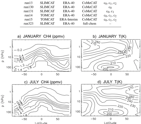
CoMeCAT coefficients have been calculated from full-chemistry runs of the global 3-D TOMCAT/SLIMCAT CTM, similar to the method employed in Monge-Sanz et al. (2011) for the calculation of coefficients for a stratospheric ozone scheme. To calculate the coefficients, a TOMCAT box model version was used. The box model configuration is identical to the 3-D CTM (chemical descriptions, grid resolution etc.) except that it does not consider transport processes. The box model was initialised with the zonally averaged output of a full-chemistry simulation of the SLIMCAT 3-D model (run 323). Run 323 is a multiannual SLIMCAT run that uses a 7.5◦×7.5◦horizontal resolution and 24 vertical levels (L24). The run is driven by ERA-40 winds (Uppala et al., 2005) from 1977 to 2001 and by ECMWF operational winds from 2002 to 2006. The period chosen to initialise the box model is January to December 2004. The box model is initialised by reading input from run 323 for every month of the year 2004, and then a series of 2-day runs is performed for each month. From the initial state, five 2-day runs of the box model were carried out: one control run and four perturbation runs from the initial conditions. In these runs the chemistry was com-puted every 20 minutes. The resolution adopted for the box model is 24 latitudes, and 24 levels (from the surface up to ∼60 km), matching the resolution of the full-chemistry run used for the initialisation. The box model also uses the same chemistry module as the full SLIMCAT model.

Table 1. TOMCAT/SLIMCAT CTM runs performed with the CoMeCAT scheme and full-chemistry run323. For each run, the CTM mode

(σ-θSLIMCAT orσ-p TOMCAT) and the winds used to drive the simulation are indicated. For the runs using the CoMeCAT scheme, the terms of the parameterisation that have been active for the particular run are also included. Winds for the runs with CoMeCAT correspond to year 2000.

CTM run CTM mode Winds CH₄ Active terms

run13 SLIMCAT ERA-40 CoMeCAT c0, c1, c2

run130 SLIMCAT ERA-40 CoMeCAT c₀

run131 SLIMCAT ERA-40 CoMeCAT c0, c1 run14 TOMCAT ERA-40 CoMeCAT c0, c1, c2 run15 TOMCAT ERA-Interim CoMeCAT c0, c1, c2

run323 SLIMCAT ERA-40 full-chem –

c) JULY CH4 (ppmv) d) JULY T(K)

a) JANUARY CH4 (ppmv) b) JANUARY T(K)

Fig. 1. Zonal mean of CoMeCAT[CH4](ppmv) (left panels) and temperatureT (K) (right panels) reference terms for January (top row) and

July (bottom row) 2004. These reference terms come from the SLIMCAT CTM (see main text for details, Sect. 3.1).

Figure 1 plots the zonal mean of the reference values for [CH4] and T for January and July. Stratospheric CH4 in the full-chemistry SLIMCAT has been widely validated, and compares very well with MIPAS observations (e.g. Kouker, 2005). The temperature field corresponds to ECMWF oper-ational data for 2004 interpolated onto the CTM grid. The CoMeCAT zonal mean CH4lifetime,τ, is plotted in Fig. 2 for January, April, July and October. The minimum lifetime values are reached at∼1 hPa, and are almost 1 yr over the summer pole, where the maximum CH4 loss rate occurs. Above 1 hPa, CH4loss decreases (lifetime increases) due to the decrease in the abundance of OH. The lifetime values in Fig. 2 are in overall agreement with those in Brasseur and Solomon (2005).

c) JULY d) OCTOBER

a) JANUARY b) APRIL

Fig. 2. Altitude–latitude distribution of CoMeCAT CH4lifetimeτ(inverse of the loss rate). Values ofτare shown, in years, for (a) January,

(b) April, (c) July and (d) October.

Table 2. ECMWF runs with CoMeCAT CH4and H2O schemes. The ECMWF GCM has been used in free-running mode or in nudged mode

to reanalyses as shown. In all these runs stratospheric CH4and H2O can come from the CoMeCAT scheme, from the default ECMWF option or remain inactive, as indicated. For the runs included here the CoMeCAT scheme was not interactive with the ECMWF radiation scheme. The meteorology used for the nudged runs corresponds to year 2000.

ECMWF run GCM CH4scheme H2O scheme

fif4 Free GCM CoMeCAT ECMWF default

fi6n Free GCM CoMeCAT CoMeCAT

fif5 Free GCM none none

fh22 Nudged to ERA-40 every 6h CoMeCAT ECMWF default fh23 Nudged to ERA-Interim every 6h CoMeCAT ECMWF default

The values ofc2 (loss tendency with respect to temper-ature) are negative everywhere except in the equatorial LS (between 100 and 200 hPa) and in the Arctic summer LS (Fig. 4). The negative sign agrees with the fact that by in-creasing temperature,ki in Eq. (11) increases, which means more CH4 loss. The decrease in loss over the Arctic sum-mer (positive contours in Fig. 4c) is explained by a secondary effect, coming from decreased OH concentrations at higher temperature, that outweighs the direct temperature effect in this region.

3.2 HALOE observations of CH4and H2O

The results of the model simulations in this study have been validated against observations from the Halogen Occultation Experiment (HALOE) instrument, on board the Upper At-mosphere Research Satellite (UARS, Russell et al., 1993) of CH4(Park et al., 1996) and H2O (Harries et al., 1996). The

HALOE data used in our study correspond to the third pub-lic release v19 (W. Randel and F. Wu, personal communi-cation, 2006). These HALOE data are zonally averaged and are available for 41 latitudes (80◦N–80◦S) and 49 pressure levels (from 100 to 0.01 hPa); the monthly time series cov-ers the period November 1991–November 2005. The accu-racy for these CH4observations is better than 7 % between 1 and 100 hPa (Park et al., 1996) and 10 % for H2O measure-ments at the same altitude range. Such HALOE data have been widely validated and have been used for several model results validations (e.g. Chipperfield et al., 2002; Bregman et al., 2006; Eyring et al., 2006; Feng et al., 2007).

3.3 CoMeCAT methane distributions

-c) JULY d) OCTOBER

a) JANUARY b) APRIL

Fig. 3. Altitude–latitude distribution of the CoMeCAT loss tendency with [CH4] (coefficientc1) in units of (10−14day−1ppmv−1) for (a)

January, (b) April, (c) July and (d) October. Solid contours indicate positive values; dashed contours indicate negative values.

c) JULY d) OCTOBER

a) JANUARY b) APRIL

Fig. 4. Altitude–latitude distribution of the CoMeCAT loss tendency with temperature (coefficientc2) in units of (10−16day−1K−1)for

(a) January, (b) April, (c) July and (d) October. Contours are plotted every 10 units. Solid contours indicate positive values; dashed contours

indicate negative values.

θ vertical levels) runs driven by ERA-40 winds include those using the CoMeCAT scheme for CH4(run13, run130, run131) and one full chemistry run (run323). There are also two TOMCAT (σ-p vertical coordinate) runs which imple-ment the CoMeCAT scheme, one driven by ERA-40 and

c)

c)

b)

b)

a)

a)

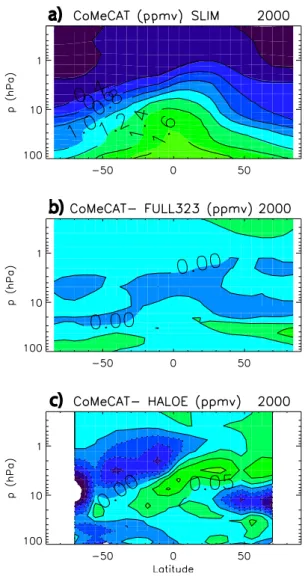
Fig. 5. Annual mean for year 2000 of (a) zonally averaged CH4

distributions (ppmv) from the CoMeCAT scheme in the CTM run13, (b) differences between CoMeCAT and full-chemistry run of SLIMCAT (run323) and (c) differences between CoMeCAT and HALOE observations. The model simulations use ERA-40 winds. Contour values are 0.20 ppmv for (a) and 0.05 ppmv for (b) and (c). Colour scale in (a) goes from larger concentrations (darkest green) to smaller concentrations (darkest blue), while for (b) and (c) the colour scale indicates most positive differences (in darkest green) and most negative differences (in darkest blue). HALOE observa-tions are available for the latitudinal range 80◦S–80◦N.

model simulations. A series of runs with the ECMWF GCM (IFS) has also been carried out using the CoMeCAT scheme (Table 2). The runs were performed with the Cy36r1 model version with a T159 horizontal resolution (1.125◦) and 60 vertical levels up to 0.1 hPa.

3.3.1 CoMeCAT against full chemistry

Figure 5 shows the annual mean zonal average CH4 concen-trations from the parameterisation in run13, as well as

dif-ferences with the full-chemistry run323 and with HALOE CH4measurements above 100 hPa. Results in Fig. 5 corre-spond to year 2000, which is different to the year used to compute the CoMeCAT coefficients (meteorological condi-tions of 2004, Sect. 3.1). Both simulacondi-tions, CoMeCAT and full chemistry used the same ECMWF ERA-40 winds. The CoMeCAT parameterisation is able to capture all general features and variability. There are differences over the trop-ics above 10 hPa, where CoMeCAT CH4concentrations are slightly smaller (up to 0.05 ppmv), as well as in LS high lat-itudes, where CoMeCAT simulates up to 0.10 ppmv more than SLIMCAT full chemistry over the Arctic. The overall agreement with HALOE is good; modelled concentrations, both CoMeCAT and full chemistry, are up to 0.20 ppmv smaller than HALOE in the most upper levels (above 20 hPa) in the Southern Hemisphere (SH), with maximum differ-ences concentrated around 10 hPa at high latitudes in both hemispheres. CoMeCAT simulates more CH4than observed over the tropical mid-stratosphere and most upper levels at high Northern Hemisphere (NH) latitudes. The differences between the two modelled CH4 fields (CoMeCAT and full chemistry) are smaller than the differences between the mod-elled fields and HALOE observations.

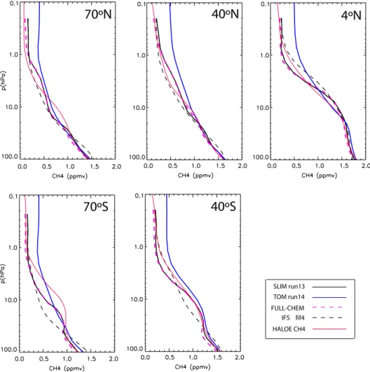
Annually averaged (year 2000) vertical CH4distributions from CoMeCAT and from the full-chemistry run 323 be-tween 100 and 0.2 hPa are shown in Fig. 6 for five different latitudes. The CoMeCAT vertical distribution in the SLIM-CAT run (run13) agrees well with the full-chemistry run. The most significant differences occur above 1 hPa, where CoMeCAT overestimates CH4 by up to 0.1 ppmv, and be-low 30 hPa, where the parameterisation, especially at south-ern mid-latitudes, results in smaller concentrations than the full chemistry (up to 0.05 ppmv smaller). CoMeCAT in the TOMCAT run (run14) is also in good agreement with full chemistry in the LS, but in the middle and upper stratosphere it simulates more CH4 than the SLIMCAT run13. Above 1 hPa differences of up to 0.25 ppmv occur widely and run14 results in up to 0.40 ppmv more than run323 in the highest levels at tropical latitudes, the reason for these differences is the too fast vertical transport in the TOMCAT run (Monge-Sanz et al., 2007).

70ºS

70ºN

40ºS

40ºN

4ºN

SLIM run13 TOM run14

HALOE CH4 FULL-CHEM IFS fif4

Fig. 6. Annually averaged CH₄distributions (ppmv) for year 2000 from the CoMeCAT scheme in SLIMCAT run13 (solid black line),

TOMCAT run14 (blue line) and in the ECMWF GCM (dashed black line) run fif4 (Table 2) for the latitudes 70◦N, 40◦N, 4◦N, 70◦S and 40◦S (as labelled). HALOE observations have also been included (red line), as well as the CTM full-chemistry run323 (red dashed line).

latitudes above 20 hPa. Thec2term (i.e. the indirect T effect) in run13 reduces the CH4values between 30 and 3 hPa with respect to run131 (Fig. 7). In the uppermost levels (above 2 hPa), thec2term acts to increase the concentrations, espe-cially over mid- and low latitudes.

3.3.2 CoMeCAT in the GCM

The ECMWF runs were initialised with the CH4 reference field from the CTM. Figure 6 shows annually averaged CH4 vertical distributions from the CoMeCAT scheme in the CTM and in the ECMWF GCM (run fif4). Two differ-ent CTM runs are included: the default SLIMCAT (σ-θ) one (run13) and also one TOMCAT (σ-p) run (run14) for a better comparison against the ECMWF runs, which, like the GCM, also uses aσ-p vertical coordinate. The overall agreement in the LS (up to 10 hPa) is good between all runs and obser-vations (with differences smaller than 0.1 ppmv); larger dif-ferences occur above 10 hPa. At the highest levels the agree-ment with observations is good for fif4 and SLIMCAT run13,

70ºS

70ºN

40ºS

40ºN

4ºN

run131-run130

run13 -run131

Fig. 7. Annual average (year 2000) of the profiles for CH4differences (ppmv) between run131 and run130 (black line) and between run13

and run131 (blue line). Run13 uses the full parameterisation as in Eq. (12), run130 uses only the first term (c0in Eq. (12)) and run131 uses only the c0and c1terms of the scheme. All runs are driven by ERA-40 reanalyses.

a significant noise reduction (e.g. Liu et al., 2010; Ploeger et al., 2011), in agreement with our comparison in Fig. 6.

4 Stratospheric H2O distributions from CoMeCAT

4.1 CoMeCAT H2O distributions within the CTM

To obtain CoMeCAT water distributions with the SLIMCAT CTM, the humidity field from the ECMWF analysis is used in the troposphere, while in the stratosphere the relation de-scribed in Eq. (14) is used to obtain H2O tendencies from CoMeCAT. In the tropics (15◦S–15◦N) H2O is taken from the ECMWF analyses for levels below the level at which the minimum temperature is reached; outside the tropics the ECMWF H2O field is used when the absolute potential vor-ticity (PV) is less than 2 PVU2and the potential temperature (θ) less than 380 K, or ifθ is less than 300 K. For all other 2_{PVU is potential vorticity unit and its value is} 1 PVU = 10−6m2s−1K kg−1.

levels we use the CoMeCAT scheme to compute the strato-spheric tendencies of water vapour.

e) HALOE avg 2000

c) fif5 (ctrl.) avg 2000 d) fif4 (default) avg 2000 b) fi6n (comecat) avg 2000 a) CTM CoMeCAT avg 2000

Fig. 8. H2O (ppmv) cross sections averaged over year 2000 obtained from (a) CoMeCAT in the SLIMCAT run13, (b) CoMeCAT in ECMWF

run fi6n, (c) ECMWF control run fif5, (d) ECMWF default scheme in run fif4 and (e) HALOE instrument. Colour scale goes from larger concentrations (orange) to smaller concentrations (dark blue). Contour interval is 0.5 ppmv. HALOE observations are available for the latitudinal range 80◦S–80◦N.

4.2 CoMeCAT H2O distributions in the GCM

The default ECMWF (currently operational) stratospheric water scheme and H2O obtained from the CoMeCAT CH4 in the ECMWF runs have been compared against HALOE observations and H2O from CoMeCAT in the CTM. The same ECMWF runs used to obtain results in Sect. 3.3 have been used to parameterise stratospheric H2O (Table 2). The initial value for the H2O tracer in the ECMWF runs was 7.0×10−6−2[CH4]. Figure 8 shows H2O cross sections av-eraged over the year 2000 obtained from CoMeCAT in the ECMWF model (run fi6n). Also shown in the same figure are H2O from the default ECMWF scheme (run fif4) and from an ECMWF control run (fif5) in which no water source scheme is used in the stratosphere.

4.2.1 ECMWF default H2O scheme

which also makes the concentration gradients realistic. Com-pared to the CTM run and to HALOE observations, the ECMWF H2O distributions show a negative bias in the trop-ics around 100 hPa; H2O in the ECMWF run is 2.5 ppmv smaller than in the CTM run (Fig. 8a) and 2.0 ppmv smaller than HALOE observations (Fig. 8e). This bias is present in all three ECMWF simulations, independent of the scheme used to obtain stratospheric H2O, which indicates a charac-teristic of this version of the ECMWF GCM that will require further investigation.

4.2.2 ECMWF new H2O scheme from CoMeCAT

The distribution of water from the CoMeCAT scheme imple-mented in the ECMWF model (run fi6n) is shown in Fig. 8b. Compared to the performance of the same scheme in SLIM-CAT (Fig. 8a), the ECMWF run shows smaller H2O val-ues (up to 0.5 ppmv lower above 10 hPa). The SLIMCAT run is closer to the HALOE distribution (Fig. 8e). In the ECMWF model, CoMeCAT produces vertical distributions of H2O similar to those from the IFS default scheme, except at high levels (above 10 hPa), where CoMeCAT can simu-late up to 0.5 ppmv more H2O at some latitudes (Fig. 8). The differences between the CoMeCAT H2O distributions in the CTM and the ECMWF runs partly arise from the fact that fi6n comes from the free-running GCM while the SLIMCAT run is forced by 6-hourly ERA-40 analyses. This last factor conditions the concentrations entering through the tropopause, as it is the analysed humidity field that is adopted for the troposphere in the CTM runs. ERA-40 shows a 10 % wet bias with respect to HALOE in the LS (Oikonomou and O’Neill, 2006). The too large H2O concentrations that en-ter the CoMeCAT scheme from the tropopause are accumu-lated throughout the entire stratosphere, causing the CoMe-CAT CTM run to show larger concentrations than HALOE (Fig. 8a). On the other hand, the problems shown by the ECMWF default H2O scheme in previous analysis versions, e.g. in ERA-40 (Uppala et al., 2005), have been partially overcome due to a more realistic transport in the more re-cent ECMWF model versions (like the one used for this run fif4).

5 Effects of GCM nudging on stratospheric tracers transport

The use of nudged GCMs is increasing over recent years as a potential way to make these models closer to the real at-mosphere (Jeuken et al., 1996; Schmidt et al., 2006; Telford et al., 2008; Douville, 2009). Such an approach consists of relaxing, or nudging, the GCM dynamical fields towards me-teorological (re)analyses so that, ifM is the model opera-tor andGthe nudging parameter, the evolution of a certain

model variablexis given by

∂x

∂t =M(x+G(xan−x)), (15)

Nudging improves temperature and fast horizontal wind fields in the GCM; however, the impact of nudging on the slow stratospheric meridional circulation has not been widely tested yet. Until now, most published studies on GCM nudg-ing have focused on nudgnudg-ing effects on dynamical fields (e.g. Telford et al., 2008; Douville, 2009), neglecting the effects this has on the distribution of chemical tracers in the strato-sphere. A few studies have evaluated the ability of nudged models to simulate the distribution of stratospheric tracers compared to observations (e.g. van Aalst et al., 2004; Jöckel et al., 2006; Lelieveld et al., 2007). Here we evaluate nudg-ing effects on stratospheric circulation thanks to the inclu-sion of CoMeCAT as a suitable stratospheric transport tracer in the ECMWF GCM. The CoMeCAT tracer has allowed us to evaluate, in online runs, the effects that nudging the GCM to reanalyses has on stratospheric transport compared to the free-running GCM and to corresponding offline CTM runs. To the best of our knowledge, the present study is the first one to tackle this kind of comparison.

Two nudged IFS simulations have been performed for this transport evaluation: experiments fh22 and fh23 (Table 2) have been produced with the same GCM version and the same CoMeCAT parameterisation as the free-running GCM simulation fi6n. However, in fh22 the dynamical variables are relaxed to ERA-40 values (year 2000), and in fh23 they are relaxed to ERA-Interim.

All dynamical variables are nudged and the nudging is ap-plied to the full vertical range of the IFS model. The relax-ation is done instantaneously every 6 h. Even if this nudging procedure is stronger than the nudging usually applied within other GCMs, it needs to be taken into account that we are nudging the ECMWF GCM with ECMWF reanalyses. The fact that the GCM is the same one used to produce the re-analyses helps to reduce inconsistencies, which in other cases needs to be done by applying weaker nudging strategies.

b) CoMeCAT free IFS (fi6n)

d) CoMeCAT IFS nudged ERA-40 (fh22) a) CoMeCAT SLIMCAT (run13)

c) CoMeCAT TOMCAT ERA-40 (run14)

e) CoMeCAT TOMCAT ERA-Int (run15) f ) CoMeCAT IFS nudged ERA-Int (fh23)

Fig. 9. Annually averaged zonal CH4distributions (ppmv) for year 2000 from the CoMeCAT tracer in (a) the SLIMCAT CTM run13, (b)

the free-running GCM fi6n, (c) the TOMCAT run14 forced by ERA-40 fields, (d) the GCM run fh22 nudged to ERA-40, (e) the TOMCAT run15 forced by ERA-Interim and (f) the GCM run fh23 nudged to ERA-Interim. Colour scale goes from larger concentrations (dark green) to smaller concentrations (dark blue). Contour interval is 0.20 ppmv.

closer to the transport features in ERA-40, with the associ-ated known problems. The TOMCAT run forced by ERA-Interim brings the CH4 distribution closer to that from the SLIMCAT run. Similarly, the GCM run nudged to ERA-Interim (fh23) is in better agreement with the SLIMCAT run and the free-running GCM than fh22. This also indicates that the effect the too fast stratospheric transport in ERA-40 had on stratospheric tracers is significantly improved in ERA-Interim.

In the nudged GCM, an upper limit to the quality of the dynamical fields is set by the meteorological data used for the nudging: when ERA-40 fields are used, the nudged GCM shows the same problems as the offline CTM driven by the same ERA-40 fields, while the distribution of the strato-spheric tracers improves in a similar way in the TOMCAT ERA-Interim run and in the GCM nudged to ERA-Interim fields. The experiments in this section therefore show not only the potential of CoMeCAT as an internal tracer for stratospheric transport but also provide an assessment of a

GCM nudged to the ERA-40 and ERA-Interim reanalyses. Our assessment shows that the GCM nudged to these mete-orological series exhibits similar features to the CTM driven by the same meteorological fields, exposing the potential limitations of nudged GCM runs for tracer transport applica-tions, compared to the less computationally expensive CTM runs.

6 Stratospheric methane, radiation and temperature

had in the stratosphere. They used the Canadian AGCM3 general circulation model (McFarlane et al., 1992) with a simplified treatment for the chemical loss of N2O, CH4, CFC-11 and CFC-12. Curry et al. (2006) found a general cooling of the stratosphere compared to the use of well-mixed concentrations for these GHGs, mainly caused by the additional H2O resulting from the CH4oxidation; they also found increases in temperature in the upper winter strato-sphere (up to 8 K over the pole).

6.1 Stratospheric temperatures

In past versions of the IFS GCM, a global CH4 value of 1.72 ppmv was used by the ECMWF radiation scheme (Bechtold et al., 2009); such a value is typical of tropospheric levels, and was shown by Monge-Sanz (2008) to cause tem-perature biases in the upper stratosphere compared to the use of the CoMeCAT tracer coupled to the ECMWF radiation scheme. In the IFS version used in the present study, the de-fault CH4 field included in the radiation scheme is a two-dimensional climatology derived from the reanalysis of the Global and regional Earth-system Monitoring using Satellite and in-situ data project (GEMS, Hollingsworth et al. 2008). In order to evaluate the impact that CoMeCAT has on the ECMWF temperature field, compared to the default climatol-ogy, CoMeCAT has been made interactive with the ECMWF radiation scheme, and temperature changes in the GCM have been examined. For this, three sets of simulations have been performed with the CoMeCAT parameterisation in IFS:

(i) one in which CoMeCAT CH4 is not interactive with the radiation scheme (ft46), and therefore the radiation scheme still sees the climatological GEMS CH4fields; (ii) one with CoMeCAT CH4 interactive with the

radia-tion scheme (ft5b);

(iii) one with CoMeCAT CH4 interactive with the radia-tion scheme and with activated CoMeCAT CH4 oxida-tion to H2O (ftjs).

Simulations ft46 and ft5b use the operational ECMWF CH4 oxidation to H2O as described in www.ecmwf.int/ research/ifsdocs/CY36r1/PHYSICS/IFSPart4.pdf. Each of these GCM simulations covers the period 1996–2000 and each 1 yr run consists of four 1 yr forecasts (with an addi-tional spin-up period of 2 months) started 30 h apart: 1 Jan-uary at 00:00 UTC, 2 JanJan-uary at 06:00 UTC, 3 JanJan-uary at 12:00 UTC and 4 January at 18:00 UTC. The different start-ing hours (00:00, 06:00, 12:00 and 18:00 UTC) ensure that the diurnal cycle is properly sampled, minimising potential biases resulting from the fact that model output is archived every 24 h. The radiation calculations are performed every hour, which is also the time step of the model integration, using the ECMWF operational radiation scheme (Morcrette et al., 2008).

80O_{N 60}O_{N 40}O_{N 20}O_{N 0}O ₂₀O_{S 40}O_{S 60}O_{S 80}O_S

1000800 600 500 400 300 200 10080 60 50 40 30 20 108 6 5 4 3 2 1 0.8 0.6 0.5 0.4 0.3 0.2

a) Difference in T ft5b-ft46 JJA 1996-2000

-3 -2 -1 -0.5 -0.2 -0.1 0.1 0.2 0.5 1 2 3

80O_{N 60}O_{N 40}O_{N 20}O_{N 0}O ₂₀O_{S 40}O_{S 60}O_{S 80}O_S

1000800 600 500 400 300 200 10080 60 50 40 30 20 108 6 5 4 3 2 1 0.8 0.6 0.5 0.4 0.3 0.2

b) Difference in T ftjs-ft5b JJA 1996-2000

-3 -2 -1 -0.5 -0.2 -0.1 0.1 0.2 0.5 1 2 3

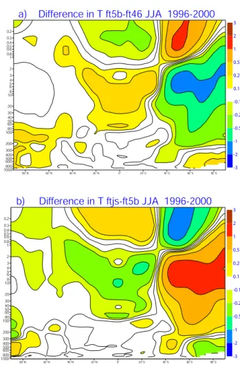
Fig. 10. Differences in temperature (K) averaged over

June-July-August (JJA) 1996–2000 between the ECMWF runs (a) ft5b (CoMeCAT CH4 in the radiation scheme) and ft46 (GEMS CH4 climatology in the radiation scheme); (b) run ftjs (CoMeCAT CH4 and H2O in the radiation scheme) and run ft5b (CoMeCAT CH4in the radiation scheme). Colour scale goes from most negative differ-ences (dark blue) to most positive differdiffer-ences (dark red).

latitudes. The value of the differences outside the winter high latitudes is within the standard deviation of temperature for the 1996–2000 period over this region for the two IFS runs. To obtain more information, longer runs would be required, which were beyond the resources available for this study. Nevertheless, the temperature differences in Fig. 10a agree with the differences in the CH4fields of both runs (ft5b-ft46) shown in Fig. 11. The CoMeCAT CH4concentrations for the JJA average over the period 1996–2000 are larger than in the GEMS climatology for the tropics at levels between 0.5 and 100 hPa (Fig. 11); larger concentrations result in warmer temperatures for that region, and a corresponding tempera-ture effect of opposite sign above the same region (as it can be seen in Fig. 10a). Analogously, the smaller CoMeCAT CH4stratospheric concentrations over the SH, reinforced by the larger CoMeCAT CH4tropospheric values, have a cool-ing effect with respect to the use of the GEMS climatology in the low and mid-stratosphere.

Figure 10b shows the June-July-August (JJA) averaged differences in temperature in the ECMWF model when both CH4and H2O from CoMeCAT are interactive with the radi-ation scheme (run ftjs) and when only CoMeCAT CH4 in-teracts with radiation (run ft5b). The effect the H2O con-centrations from CoMeCAT CH4oxidation have on temper-ature is of up to 1.0 K decrease over the tropical mid/low stratosphere, and a warming of the SH mid/high latitudes be-tween 1 and 200 hPa. The temperature differences in Fig. 10b are larger than the values for the standard deviation of tem-perature of the corresponding runs (ftjs, ft5b), which shows that the effects on temperature from the combined CoMeCAT CH4and H2O fields produce a signal stronger than the model internal variability. These results highlight the advantage of including schemes for radiative gases that are consistent with each other (like CoMeCAT CH4and H2O), compared to the use of different climatologies/schemes for each gas (where effects can be cancelled or enhanced for the wrong reasons).

6.2 Radiative forcing

Further calculations of radiative effects of the CoMeCAT CH4 distribution have been performed with the offline ver-sion of the Edwards–Slingo (E-S) radiative transfer model (Edwards and Slingo, 1996) with a 2.5◦ horizontal resolu-tion and 23 pressure levels. The vertical levels in our E-S model runs match those of the original archiving of ERA-40 fields on pressure levels3. This state-of-the-art radiative model uses nine bands in the longwave and six bands in the shortwave and a delta-Eddington two-stream scattering solver at all wavelengths. The E-S model employs a monthly averaged climatology based on ERA-40 data for temperature, ozone and water vapour. Monthly mean climatological cloud fields and surface albedo (averaged over the period 1983–

3_{www.ecmwf.int/products/data/archive/descriptions/e4/oper/}

an/pl/2.5/index.html

80O_{N 60}O_{N 40}O_{N 20}O_{N 0}O ₂₀O_{S 40}O_{S 60}O_{S 80}O_S

1000800 600 500 400 300 200 10080 60 50 40 30 20 108 6 5 4 3 2 1 0.8 0.6 0.5 0.4 0.3 0.2

Difference in CH4 (1.E-8 kg/kg) JJA 1996-2000

-35 -25 -15 -10 -7 -5 -3.5 -2 -1 1 2 3.5 5 7 10 15 25 35

Fig. 11. Differences in the CH4concentrations (10−8kg kg−1)

be-tween the CoMeCAT distribution and ECMWF GEMS climatology in the radiation scheme, averaged for June-July-August (JJA) 1996– 2000. Colour scale goes from most negative differences (dark blue) to most positive differences (dark red).

2005) are taken from the International Satellite Cloud Clima-tology Project (ISCCP) archive (Rossow and Schiffer, 1999). Clouds are added to three vertical levels, corresponding to low, middle and high clouds. The version of the E-S model we use here has been recently tested in Forster et al. (2011).

The CoMeCAT radiative effect (RE) has been evaluated for each calendar month by taking the differences between three runs of the E-S radiation code: (i) one control run (“ctrl”) using a global 3-D constant CH4value of 1.80 ppmv for CH4 (the same for every calendar month), (ii) one per-turbed run (“come”) taking the CH4 distribution from the CoMeCAT CH4field in the CTM run13 and (iii), one second perturbed run (“gems”) using the same CH4GEMS climatol-ogy as the ECMWF model currently uses by default.

Fig. 12. Annually averaged net radiative forcing (mW m−2) in-duced by using the CoMeCAT CH4(a) instead of a default constant value of 1.80 ppmv in the Edwards–Slingo (E-S) radiation model (upper panel) and (b) instead of the GEMS climatology for CH₄ in the E-S model (bottom panel). See main text (Sect. 6.2) for de-tails about the model runs used for these calculations. In the colour scale, blue is for negative radiative effect (cooling), and red for pos-itive radiative effect (warming).

methane concentrations will overestimate surface warming globally. The use of a constant CH4profile is still the default option in offline radiative models like the E-S model, which are widely used for climate research. Figure 12a therefore shows the importance of an improved stratosphere in radia-tive forcing calculations, with respect to the standards cur-rently used for climate studies.

Figure 12b shows the annual mean values of the net RE differences, between the “come” run using the CoMe-CAT CH4 field and the “gems” run using the same CH4 GEMS climatology as ECMWF currently uses. There is an overall warming effect at all latitudes with a global mean average value of 30 mW m−2; maximum values of up to 100 mW m−2are found over the tropics. The only exception

Fig. 13. Annually averaged cross section for the differences in the

CH4 concentrations (10−6kg kg−1) between the CoMeCAT dis-tribution and the ECMWF GEMS climatology; these differences correspond to the radiative effect (RE) shown in the lower panel of Fig. 12. Colour scale goes from most negative differences (dark blue) to most positive differences (dark red).

to the warming is the Antarctic continent, where cooling of up to 30 mW m−2is obtained when using the CoMeCAT field instead of the GEMS climatology. The distribution of these radiative effects is very dependent on the altitude at which the differences in CH4concentrations between the two runs are found (Riese et al., 2012). Figure 13 shows the cross section of CH4differences corresponding to the calculations shown in Fig. 12b. Even if the largest differences between CoMe-CAT and GEMS are found above 100 hPa – that is, where the influence on radiative effects is not the largest (Riese et al., 2012) – such differences are still modifying the effects of the differences in CH4found in lower levels, including tro-pospheric levels. Results in Figs. 12b and 13 show that, in our runs, effects due to differences below the tropopause are compensated (or enhanced) by the differences found in the SH lower stratosphere (or the NH mid-stratosphere).

7 Conclusions

A new CH4parameterisation scheme (CoMeCAT) has been developed for the stratosphere, and tested within a 3-D CTM and a 3-D GCM. The scheme has the advantage of parame-terising both stratospheric CH4and H2O in a consistent and efficient way.

compared to HALOE by up to 0.3 ppmv at altitudes around 10 hPa. CoMeCAT also performs well in the ECMWF GCM, producing realistic CH4 distributions. The CH4 time ten-dency obtained from CoMeCAT has been used in both mod-els (CTM and GCM) to parameterise the source of strato-spheric water. The H2O distributions obtained from CoMe-CAT in the CTM runs are in good agreement with HALOE observations, except for a wet bias in the LS region of ∼0.6 ppmv. This is at least partly due to the use of ERA-40 humidity values in the troposphere, which show a wet bias at the tropopause. In the ECMWF model the CoMeCAT water approach performs well. ECMWF CoMeCAT H2O distribu-tions show realistic spatial variability and good agreement with HALOE observations, except for a dry bias in the trop-ical lower stratosphere (of up to 2.0 ppmv).

The CoMeCAT scheme has also provided the ECMWF GCM with a suitable tracer (CH4 tracer) for internal tests of stratospheric transport. This has allowed us to compare, for the first time, stratospheric transport in the free-running ECMWF GCM, also in two nudged configurations of the GCM and in corresponding offline CTM runs. Nudging the GCM to ERA-40 analyses produced similar CH4 distribu-tions to those obtained with the TOMCAT (σ-p) run by ERA-40. Nudging the GCM to ERA-Interim brought about im-provements, compared to the nudging to ERA-40, similar to those obtained in the TOMCAT run driven by ERA-Interim instead of ERA-40 fields. These results show that a nudged GCM incorporates the advantages and deficiencies of the analyses used, and nudging a recent version of the ECMWF IFS to ERA-40 is not recommended for applications involv-ing transport of stratospheric tracers. Our results also indi-cate that runs with nudged GCMs do not necessarily show improvement over cheaper offline CTM runs regarding the stratospheric transport of tracers.

CoMeCAT impacts on radiation and temperature have been explored with two different models. When using CoMe-CAT interactively with the ECMWF radiation scheme, the new CH4warms (up to 0.5 K) the middle stratosphere over mid/low latitudes compared to the use of the default CH4 field from the GEMS climatology. Using also CoMeCAT H2O in the radiation scheme decreases temperature over the tropical mid/low stratosphere and warms most of the SH stratosphere outside the tropics. These results show the im-portance of using distributions of CH4and H2O that are con-sistent with each other.

The CoMeCAT scheme is a more realistic treatment for stratospheric CH4 than previously included in ECMWF. As a next step, the effect of using CoMeCAT in conjunction with similar schemes for other GHGs (e.g. N2O and CFCs) in models like IFS should be investigated. In addition, in-cluding this type of CH4/H2O scheme in the ECMWF model would also enable the assimilation of CH4concentrations to be used to constrain humidity analyses in the stratosphere. In this study we have not been able to test the performance of CoMeCAT in data assimilation runs of the ECMWF model

due to limitations in resources available for this project; how-ever, this remains as a future line of research. The CoMe-CAT scheme is also a good option to represent stratospheric CH4 within the Monitoring Air Composition and Climate (MACC) project; this is now part of ongoing research at ECMWF.

The CoMeCAT scheme also opens new possibilities for climate studies. In spite of being the second-most impor-tant greenhouse gas, many climate models use only a fixed value for CH4in the stratosphere. Including a realistic CH4 profile, with latitude dependence and linked to other model variables (like temperature), is expected to produce changes to radiative forcing results in climate models. In our study, including the CoMeCAT methane distribution in the offline Edwards–Slingo (E-S) state-of-the-art radiation model has had an effect on the calculated radiative forcing values of the same order of magnitude, but of different sign, as the in-corporation of aircraft contrail formation. The use of CoMe-CAT instead of the default well-mixed approximation in the stratosphere has reduced radiative forcing values by up to 30 mW m−2over mid- and high latitudes, with a global annu-ally averaged change of−11.0 mW m−2. This implies that a realistic representation of vertical distribution of GHGs in the stratosphere is necessary to better constrain radiative forcing and climate warming projections. In this sense it can be said that the stratosphere plays a similar role to that played by the oceans: the stratosphere acts as a slowly evolv-ing boundary for the troposphere, and a realistic descrip-tion of stratospheric processes is key to increasing the accu-racy of long-term climate predictions. In addition, Solomon et al. (2010) highlighted the need for better representations of stratospheric H2O in climate models to better simulate and interpret decadal surface warming trends; the CoMeCAT scheme could also contribute in this respect. The inclusion of realistic schemes for other GHGs, like N2O and CFCs, is ex-pected to have the same type of effect as we have shown here for methane. The total net contribution of such parameterised stratospheric GHGs to temperature and radiation will need to be quantified. Future research should be done on the effects that realistic GHGs vertical distributions in the stratosphere have on temperature and radiative forcing calculations, and therefore on climate studies, as well as on the effects that a more realistic stratospheric composition has on seasonal pre-diction systems.

Acknowledgements. We thank Elias Hólm for valuable

commu-nications on the ECMWF H₂O scheme and Piers Forster for helpful discussions on the interaction of the scheme with the GCM radiation. We are also grateful to Lindsay Lee for advice on statistical analysis and to Nigel Richards for help with data files. This work has been funded by the NERC Research Award NE/F004575/1, the EU GEOMON project and the IEF Marie Curie Fellowship PIEF-GA-2010-273531.

References

Austin, J., Wilson, J., Li, F., and Vömel, H.: Evolution of Water Vapor Concentrations and Stratospheric age-of-air in Coupled Chemistry-Climate Model Simulations, J. Atmos. Sci., 64, 905– 921, doi:10.1175/JAS3866.1, 2007.

Bates, D. R. and Nicolet, M.: The photochemistry of water vapour, J. Geophys. Res., 55, 301–327, 1950.

Bechtold, P., Orr, A., Morcrette, J.-J., Engelen, R., Flemming, J., and Janiskova, M.: Improvements in the stratosphere and meso-sphere of the IFS, ECMWF Newsletter, 2009.

Brasseur, G. and Solomon, S.: Aeronomy of the Middle Atmo-sphere, Springer, Dordrecht, the Netherlands, 2005.

Bregman, B., Meijer, E., and Scheele, R.: Key aspects of strato-spheric tracer modeling using assimilated winds, Atmos. Chem. Phys., 6, 4529–4543, doi:10.5194/acp-6-4529-2006, 2006. Cariolle, D. and Déqué, M.: Southern Hemisphere Medium-Scale

Waves and Total Ozone Disturbances in a Spectral General Cir-culation Model, J. Geophys. Res., 91, 10825–10846, 1986. Cariolle, D. and Teyssèdre, H.: A revised linear ozone

photochem-istry parameterization for use in transport and general circula-tion models: Multi-annual simulacircula-tions, Atmos. Chem. Phys., 7, 2183–2196, doi:10.5194/acp-7-2183-2007, 2007.

Chipperfield, M. P.: New version of the TOMCAT/SLIMCAT off-line chemical transport model, Q. J. Roy. Meteorol. Soc., 132, 1179–1203, doi:10.1256/qj.05.51, 2006.

Chipperfield, M. P., Khattatov, B. V., and Lary, D. J.: Sequential assimilation of stratospheric chemical observa-tions in a three-dimensional model, J. Geophys. Res., 107, doi:10.1029/2002JD002110, 2002.

Collins, W., Ramaswamy, V., Schwarzkopf, M., Sun, Y., Portmann, R., Fu, Q., Casanova, S., Dufresne, J.-L., Fillmore, D., Forster, P., Galin, V., Gohar, L., Ingram, W., Kratz, D., Lefebvre, M.-P., Li, J., Marquet, P., Oinas, V., Tsushima, Y., Uchiyama, T., and Zhong, W.: Radiative forcing by well-mixed greenhouse gases: Estimates from climate models in the Intergovernmental Panel on Climate Change (IPCC) Fourth Assessment Report (AR4), J. Geophys. Res., 111, D14, D14317, doi:10.1029/2005JD006713, 2006.

Curry, C. L., McFarlane, N. A., and Scinocca, J. F.: Relaxing the well-mixed greenhouse gas approximation in climate simula-tions: Consequences for stratospheric climate, J. Geophys. Res., 111, D8, D08104, doi:10.1029/2005JD006670, 2006.

Dee, D. P., Uppala, S. M., Simmons, A. J., Berrisford, P., Poli, P., Kobayashi, S., Andrae, U., Balmaseda, M. A., Balsamo, G., Bauer, P., Bechtold, P., Beljaars, A. C. M., van de Berg, L., Bid-lot, J., Bormann, N., Delsol, C., Dragani, R., Fuentes, M., Geer, A. J., Haimberger, L., Healy, S., Hersbach, H., Hólm, E. V., Isaksen, L., Kållberg, P., Köhler, M., Matricardi, M., McNally, A. P., Monge-Sanz, B. M., Morcrette, J.-J., Peubey, C., de Ros-nay, P., Tavolato, C., Thépaut, J.-N., and Vitart, F.: The ERA-Interim reanalysis: Configuration and performance of the data assimilation system, Q. J. Roy. Meteorol. Soc., 137, 553–597, doi:10.1002/qj.828, 2011.

Dethof, A.: Aspects of modelling and assimilation for the strato-sphere at ECMWF, SPARC Newsletter, 21, 2003.

Dethof, A. and Hólm, E. V.: Ozone assimilation in the ERA-40 reanalysis project, Q. J. Roy. Meteorol. Soc., 130, 2851–2872, 2004.

Douville, H.: Stratospheric polar vortex influence on Northern Hemisphere winter climate variability, Geophys. Res. Lett., 36, 18, L18703, doi:10.1029/2009GL039334, 2009.

Edwards, J. M. and Slingo, A.: Studies with a flexible new radiation code: I. Choosing a configuration for a large scale model, Q. J. Roy. Meteorol. Soc., 122, 689–720, doi:10.1002/qj.49712253107, 1996.

Eyring, V., Butchart, N., Waugh, D. W., Akiyoshi, H., Austin, J., Bekki, S., Bodeker, G. E., Boville, B. A., Brühl, C., Chipper-field, M. P., Cordero, E., Dameris, M., Deushi, M., Fioletov, V. E., Frith, S. M., Garcia, R. R., Gettelman, A., Giorgetta, M. A., Grewe, V., Jourdain, L., Kinnison, D. E., Mancini, E., Manzini, E., Marchand, M., Marsh, D. R., Nagashima, T., Newman, P. A., Nielsen, J. E., Pawson, S., Pitari, G., Plummer, D. A., Rozanov, E., Schraner, M., Shepherd, T. G., Shibata, K., Stolarski, R. S., Struthers, H., Tian, W., and Yoshiki, M.: Assessment of temper-ature, trace species, and ozone in chemistry-climate model sim-ulations of the recent past, J. Geophys. Res., 111, D22, D22308, doi:10.1029/2006JD007327, 2006.

Feng, W., Chipperfield, M. P., Dorf, M., Pfeilsticker, K., and Ri-caud, P.: Mid-latitude ozone changes: studies with a 3-D CTM forced by ERA-40 analyses, Atmos. Chem. Phys., 7, 2357–2369, doi:10.5194/acp-7-2357-2007, 2007.

Forster, P. M. and Shine, K.: Radiative forcing and temperature trends from stratospheric ozone changes, J. Geophys. Res., 102, 841–855, 1997.

Forster, P. M., Fomichev, V. I., Rozanov, E., Cagnazzo, C., Jon-sson, A. I., Langematz, U., Fomin, B., Iacono, M. J., Mayer, B., Mlawer, E., Myhre, G., Portmann, R. W., Akiyoshi, H., Falaleeva, V., Gillett, N., Karpechko, A., Li, J., Lemennais, P., Morgenstern, O., Oberländer, S., Sigmond, M., and Shi-bata, K.: Evaluation of radiation scheme performance within chemistry climate models, J. Geophys. Res., 116, D10302, doi10.1029/2010JD015361, 2011.

Fueglistaler, S., Wernli, H., and Peter, T.: Tropical troposphere-to-stratosphere transport inferred from trajectory calculations, J. Geophys. Res., 109, D03108, doi:10.1029/2003JD004069, 2004. Gettelman, A., Hegglin, M. I., Son, S.-W., Kim, J., Fujiwara, M., Birner, T., Kremser, S., Rex, M., Añel, J. A., Akiyoshi, H., Austin, J., Bekki, S., Braesike, P., Brühl, C., Butchart, N., Chip-perfield, M., Dameris, M., Dhomse, S., Garny, H., Hardiman, S. C., Jöckel, P., Kinnison, D. E., Lamarque, J. F., Mancini, E., Marchand, M., Michou, M., Morgenstern, O., Pawson, S., Pitari, G., Plummer, D., Pyle, J. A., Rozanov, E., Scinocca, J., Shep-herd, T. G., Shibata, K., Smale, D., Teyssèdre, H., and Tian, W.: Multimodel assessment of the upper troposphere and lower stratosphere: Tropics and global trends, J. Geophys. Res., 115, D00M08, doi:10.1029/2009JD013638, 2010.

Harries, J. E., Russell, J. M., Tuck, A. F., Gordley, L. L., Purcell, P., Stone, K., Bevilacqua, R. M., Gunson, M., Nedoluha, G., and Traub, W. A.: Validation of measurements of water vapor from the Halogen Occultation Experiment (HALOE), J. Geo-phys. Res., 101, 10205–10216, 1996.

Vancoppenolle, M., Viterbo, P., and Willén, U.: EC-Earth: A Seamless Earth-System Prediction Approach in Action, B. Am. Meteor. Soc., 91, 1357–1363, doi:10.1175/2010BAMS2877.1, 2010.

Hollingsworth, A., Engelen, R. J., Textor, C., Benedetti, A., Boucher, O., Chevallier, F., Dethof, A., Elbern, H., Eskes, H., Flemming, J., Granier, C., Kaiser, J. W., Morcrette, J.-J., Rayner, P. R., Peuch, V.-H., Rouil, L., Schultz, M. G., Simmons, A. J., and the GEMS Consortium: Toward a monitoring and forecasting system for atmospheric composition: the GEMS project., B. Am. Meteor. Soc., 89, 1147–1164, doi:10.1175/2008BAMS2355.1, 2008.

Jeuken, A., Siegmund, P., Heijboer, L., Feichter, J., and Bengtsson, L.: On the Potential of assimilating meteorological analyses in a global climate model for the purposes of model validation, J. Geophys. Res., 101, 16939–16950, 1996.

Jöckel, P., Tost, H., Pozzer, A., Brühl, C., Buchholz, J., Ganzeveld, L., Hoor, P., Kerkweg, A., Lawrence, M., Sander, R., Steil, B., Stiller, G., Tanarhte, M., Taraborrelli, D., van Aardenne, J., and Lelieveld, J.: The atmospheric chemistry general circulation model ECHAM5/MESSy1: consistent simulation of ozone from the surface to the mesosphere, Atmos. Chem. Phys., 6, 5067– 5104, doi:10.5194/acp-6-5067-2006, 2006.

Jones, R. L. and Pyle, J. A.: Observations of CH4 and N2O by the Nimbus 7 SAMA: A comparison with in situ data and two-dimensional numerical model calculations, J. Geophys. Res., 89, 5263–5279, 1984.

Kinnersley, J. S. and Harwood, R. S.: An isentropic two-dimensional model with an interactive parameterization of dy-namical and chemical planetary wave fluxes, Q. J. Roy. Meteorol. Soc., 119, 1167–1193, 1993.

Kouker, W.: Towards the Prediction of Stratospheric Ozone (TOPOZ III), Scientific Report. EC Contract EVK2-CT-2001-00102, European Commission, Brussels, Belgium, 2005. Krüger, K., Tegtmeier, S., and Rex, M.: Long-term climatology

of air mass transport through the Tropical Tropopause Layer (TTL) during NH winter, Atmos. Chem. Phys., 8, 813–823, doi:10.5194/acp-8-813-2008, 2008.

Lelieveld, J., Brühl, C., Jöckel, P., Steil, B., Crutzen, P. J., Fis-cher, H., Giorgetta, M. A., Hoor, P., Lawrence, M. G., Sausen, R., and Tost, H.: Stratospheric dryness: model simulations and satellite observations, Atmos. Chem. Phys., 7, 1313–1332, doi:10.5194/acp-7-1313-2007, 2007.

Le Texier, H., Solomon, S., and Garcia, R. R.: The role of molecular hydrogen and methane oxidation in the water vapour budget of the stratosphere, Q. J. Roy. Meteorol. Soc., 114, 281–295, 1988. Liu, Y. S., Fueglistaler, S., and Haynes, P. H.: Advection-condensation paradigm for stratospheric water vapor, J. Geo-phys. Res., 115, D24307, doi:10.1029/2010JD014352, 2010. MacKenzie, I. A. and Harwood, R. S.: Middle atmospheric

re-sponse to a future increase in humidity arising from in-creased methane abundance, J. Geophys. Res., 109, D02107, doi:10.1029/2003JD003590, 2004.

Maycock, A. C., Keeley, S. P. E., Charlton-Perez, A. J., and Doblas-Reyes, F. J.: Stratospheric circulation in seasonal forecasting models: implications for seasonal prediction, Clim. Dynam., 36, 309–321, doi:10.1007/s00382-009-0665-x, 2011.

Maycock, A. C., Joshi, M. M., Shine, K. P., and Scaife, A. A.: The circulation response to idealized changes in stratospheric

water vapor, J. Climate, 26, 545–561, doi:10.1175/JCLI-D-12-00155.1, 2013.

McCormack, J. P., Hoppel, K. W., and Siskind, D. E.: Parameter-ization of middle atmospheric water vapor photochemistry for high-altitude NWP and data assimilation, Atmos. Chem. Phys., 8, 7519–7532, doi:10.5194/acp-8-7519-2008, 2008.

McFarlane, N. A., Boer, G. J., Blanchet, J.-P., and Lazare, M.: The Canadian Climate Centre second-generation general circulation model and its equilibrium climate, J. Clim., 5, 1013–1044, 1992. Monge-Sanz, B. M.: Stratospheric Transport and Chemical Parame-terisations in ECMWF Analyses: Evaluation and Improvements using a 3-D CTM, Ph.D. thesis, School of Earth and Environ-ment, University of Leeds, Leeds, UK, 2008.

Monge-Sanz, B. M., Chipperfield, M. P., Simmons, A. J., and Up-pala, S. M.: Mean age-of-air and transport in a CTM: Com-parison of different ECMWF analyses, Geophys. Res. Lett., 34, L04801, doi:10.1029/2006GL028515, 2007.

Monge-Sanz, B. M., Chipperfield, M. P., Cariolle, D., and Feng, W.: Results from a new linear O3 scheme with embedded hetero-geneous chemistry compared with the parent full-chemistry 3-D CTM, Atmos. Chem. Phys., 11, 1227–1242, doi:10.5194/acp-11-1227-2011, 2011.

Monge-Sanz, B. M., Chipperfield, M. P., Dee, D. P., Simmons, A. J., and Uppala, S. M.: Improvements in the stratospheric transport achieved by a CTM with ECMWF (re)analyses: Identifying ef-fects and remaining challenges, Q. J. Roy. Meteor. Soc., 139, 654–673, doi:10.1002/qj.1996, 2012.

Morcrette, J.-J., Barker, H., Cole, J., Iacono, M., and Pincus, R.: Impact of a new radiation package, McRad, in the ECMWF Inte-grated Forecasting System, Mon. Weather Rev., 136, 4773–4798, doi:10.1175/2008MWR2363.1, 2008.

Oikonomou, E. K. and O’Neill, A.: Evaluation of ozone and water vapor fields from the ECMWF reanalysis ERA-40 during 1991–1999 in comparison with UARS satellite and MOZAIC aircraft observations, J. Geophys. Res., 111, D14109, doi:10.1029/2004JD005341, 2006.

Palmer, T. N., Doblas-Reyes, F. J., Weisheimer, A., and Rodwell, M. J.: Toward seamless prediction: calibration of climate change projections using seasonal forecasts, B. Am. Meteor. Soc., 89, 459–470, 2008.

Park, J., Russell, J., L.Gordley, L., Drayson, S. R., Banner, D., McInerney, J., Gunson, M. R., Toon, G., Sen, B., Blavier, J.-F., Webster, C., Zipf, E., Erdman, P., Schmidt, U., and Schiller, C.: Validation of Halogen Occultation Experiment CH₄ measure-ments from the UARS, J. Geophys. Res., 101, 10217–10240, 1996.

Ploeger, F., Fueglistaler, S., Grooß, J.-U., Günther, G., Konopka, P., Liu, Y., Müller, R., Ravegnani, F., Schiller, C., Ulanovski, A., and Riese, M.: Insight from ozone and water vapour on transport in the tropical tropopause layer (TTL), Atmos. Chem. Phys., 11, 407–419, doi:10.5194/acp-11-407-2011, 2011.

Ramanathan, V. and Dickinson, R.: The role of stratospheric ozone in the zonal and seasonal radiative energy balance of the Earth-troposphere system, J. Atmos. Sci., 36, 1084–1104, 1979. Randel, W., Wu, F., Oltmans, S. J., Rosenlof, K., and Nedoluha,

Rap, A., Forster, P. M., Jones, A., Boucher, O., Haywood, J. M., Bel-louin, N., and De Leon, R. R.: Parameterization of contrails in the UK Met Office Climate Model, J. Geophys. Res., 115, D10205, doi:10.1029/2009JD012443, 2010.

Ravishankara, A. R.: Water vapor in the lower stratosphere, Science, 337, 809–810, doi:10.1126/science.1227004, 2012.

Riese, M., Ploeger, F., Rap, A., Vogel, B., Konopka, P., Dameris, M., and Forster, P.: Impact of uncertainties in atmospheric UTLS composition and related radiative effects, J. Geophys. Res., 117, D10205, doi:10.129/2012JD017751, 2012.

Rossow, W. and Schiffer, R.: Advances in understanding clouds from ISCCP, B. Am. Meteorol. Soc., 80, 2261–2288, 1999. Russell, J. M., Gordley, L. L., Park, J. H., Drayson, S. R., Hesketh,

W. D., Cicerone, R. J., Tuck, A. F., Frederick, J. E., Harries, J. E., and Crutzen, P. J.: The Halogen Occultation Experiment, J. Geo-phys. Res., 98, 10777–10797, 1993.

Scaife, A., Spangehl, T., Fereday, D., Cubasch, U., Lange-matz, U., Akiyoshi, H., Bekki, S., Braesicke, P., Butchart, N., Chipperfield, M., Gettelman, A., Hardiman, S., Rozanov, M. M. E., and Shepherd, T.: Climate change projections and stratosphere-troposphere interaction, Climate Dyn., 38, 2089– 2097, doi:10.1007/s00382-011-1080-7, 2012.

Schmidt, G., Ruedy, R., Hansen, J., Aleinov, I., Bell, N., Bauer, M., Bauer, S., Cairns, B., Canuto, V., Cheng, Y., Del Genio, A., Falu-vegi, G., Friend, A., Hall, T., Hu, Y., Kelley, M., Kiang, N., Koch, D., Lacis, A., Lerner, J., Lo, K., Miller, R., Nazarenko, L., Oinas, V., Perlwitz, J., Perlwitz, J., Rind, D., Romanou, A., Russell, G., Sato, M., Shindell, D., Stone, P., Sun, S., Tausnev, N., Thresher, D., and Yao, M.-S.: Present day atmospheric simulations using GISS Model: Comparison to in-situ, satellite and reanalysis data, J. Climate, 19, 153–192, 2006.

Simmons, A. J., Untch, A., Jakob, C., Kållberg, P., and Undén, P.: Stratospheric water vapour and tropical tropopause temperatures in ECMWF analyses and multi-year simulations, Q. J. Roy. Me-teorol. Soc., 125, 353–386, 1999.

Solomon, S., Rosenlof, K. H., Portmann, R. W., Daniel, J. S., Davis, S. M., Sanford, T. J., and Plattner, G.-K.: Contributions of strato-spheric water vapor to decadal changes in the rate of global warming, Science, 327, 1219–1223, 2010.

Tegtmeier, S., Krüger, K., Wohltmann, I., Schoellhammer, K., and Rex, M.: Variations of the residual circulation in the Northern Hemispheric winter„ J. Geophys. Res., 113, D16109, doi:10.1029/2007JD009518, 2008.

Telford, P. J., Braesicke, P., Morgenstern, O., and Pyle, J. A.: Tech-nical Note: Description and assessment of a nudged version of the new dynamics Unified Model, Atmos. Chem. Phys., 8, 1701– 1712, doi:10.5194/acp-8-1701-2008, 2008.

Uppala, S. M., Kållberg, P. W., Simmons, A. J., Andrae, U., Bech-told, V. D. C., Fiorino, M., Gibson, J. K., Haseler, J., Hernandez, A., Kelly, G. A., Li, X., Onogi, K., Saarinen, S., Sokka, N., Al-lan, R. P., Andersson, E., Arpe, K., Balmaseda, M. A., Beljaars, A. C. M., Berg, L. V. D., Bidlot, J., Bormann, N., Caires, S., Chevallier, F., Dethof, A., Dragosavac, M., Fisher, M., Fuentes, M., Hagemann, S., Hólm, E., Hoskins, B. J., Isaksen, L., Janssen, P. A. E. M., Jenne, R., McNally, A. P., Mahfouf, J.-F., Mor-crette, J.-J., Rayner, N. A., Saunders, R. W., Simon, P., Sterl, A., Trenberth, K. E., Untch, A., Vasiljevic, D., Viterbo, P., and Woollen, J.: The ERA-40 Re-analysis, Q. J. Roy. Meteorol. Soc., 131, 2961–3012, doi:10.1256/qj.04.176, 2005.