Is There a County Border Effect in Spatial Income Differences in Hungary?

IS THERE A COUNTY BORDER EFFECT IN SPATIAL INCOME

DIFFERENCES IN HUNGARY?

T

AMÁS DUSEK

ABSTRACT – The economic and social importance of administrative borders can be examined from the point of view of internal homogeneity and external heterogeneity of the delimited spatial units and of the effect on the intensity of spatial interactions. This paper deals with the first question. Hungarian county borders can be treated as strict limits from the administrative point of view. However, choropleth maps with county borders can suggest that county borders are strict limits for the social and economic indicators too. It is a conceptually interesting question, whether presenting data at county level is justified by the significant differences of various indicators along the county borders or if it is determined only by the availability of data. The aim of this study is to examine empirically the existence or non-existence of the county border effect by the example of spatial distribution of personal incomes in Hungary. The analysis is possible due to the availability of personal income data at the level of more than 3,000 Hungarian settlements. The results show that county borders have effect only in those cases where the border is determined by a physical geographical barrier, namely the Danube River and Lake Balaton. The settlements are more similar to the close settlements of a neighbouring county than to the average of its own county.

Keywords: border effect, administrative border, spatial income differences, Hungary

INTRODUCTION

The economic and social importance of administrative borders can be examined from the point of view of internal homogeneity and external heterogeneity of the delimited spatial units and of the effect on the intensity of spatial interactions. This paper deals with the first question. Hungarian county borders can be treated as strict limits from the administrative point of view, because Hungarian counties have important public administration tasks. The middle level administrative traffic flow is directed from the periphery of the counties to the capital city of the counties. County borders have impact on road structure, because road maintenance and building of lower level inter-settlement roads are managed by county road offices (Kanalas and Kiss, 2006). Roads across the county borders are sparser than the average road density. The spatial structure of bus companies are organized also according to the county system: each county has an own bus company with lines often terminated in settlements at the county border. These factors maybe have a discouraging effect on spatial interactions between counties, but in lack of empirical data about the traffic flows, it is not possible to analyze this question.

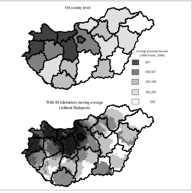
However, choropleth maps of various attribute characteristics depicted with county borders, can suggest that county borders mean strict limits for the social and economic indicators too. A common example for these indicators is the spatial differences of personal incomes (Figure 1). Personal income belongs to the persons, who are mobile, but can be localized according to their home address. The observational unit is therefore the persons, and the most basic possible spatial unit for the spatial analysis would be the home. For practical reasons and due to the statistical data collection, the smallest possible spatial units are the settlements or small precincts (residential zones, districts) inside

1

The paper was presented at the 52th Congress of the European Regional Science Association Bratislava, Slovakia, 21-25 August 2012.

2

the bigger settlements (towns and cities). However, the most detailed spatial division is in many times not the desirable one if someone is interested in the spatial differences of a larger area. For example, spatial differences inside Hungary are often analyzed on county level (19 counties and Budapest); the USA can be analyzed with 50 States, Germany with 16 Lands, Mexico with 31 States, Switzerland with 26 cantons. These spatial divisions are not arbitrary from administrative and legal point of view, but may be arbitrary from the point of view of analyzed economic or social indicators. It is a conceptually interesting question whether presenting data at a middle level administrative unit (county, state or canton) is justified by the significant differences of various indicators along the administrative unit borders or if it is determined only by the availability of data or by tradition and custom.

262-293

-262

Average personal income (1000 Forint, 2000)

367-330-367

293-330 On county level

With 40 kilometers moving average (without Budapest)

Figure 1.Average personal income, 2000

Source: Hungarian Central Statistical Office

intra-county differences. The aim of this study is to examine empirically the existence or non-existence of the county border effect by the example of spatial distribution of personal incomes in Hungary. The analysis is possible due to the availability of personal income data at the level of more than 3,000 Hungarian settlements.

The speciality of the research can be found in the fact, that intra-country analysis of this type of question is extremely rare. We do not have knowledge of the same type of research just of researches that have some common conceptual parts to our approach. For example, abundant literature exists about the border effect on price differences or everyday items between countries (Pásztor, Pénzes, 2013). There are several analyses on the disparities between various border regions (Nagy, 2013; Pénzes, Molnár, 2007). Smaller, but rapidly increasing is the literature about intra-country price differences (Zsibók, Varga, 2009; Zsibók, 2011; a survey can be found in Márkusné Zsibók, 2012). Most of these studies treat regions as points and therefore intra-region differences and distance effect are not taken into account. Border effect of counties is analysed by Bujdosó (2004), but for interregional flows and not for attribute characteristics of border regions. Fábián (2008) deals with comparison of personal incomes of border regions and non-border regions in Western Hungary. Her aim was also different from ours, because she did not analyse the possible border effect.

In the first part of the paper, the conceptual questions about the delimitation of county border areas are presented. The second part deals with the empirical analysis. In this case, comparison will be made between the personal incomes of settlements along the county borders to the following areas: average of own county, average of neighbouring county, average of neighbouring settlements, average of neighbouring settlements in own county, and average of neighbouring settlements in neighbouring county. Then, the neighbourhood of county border settlement will be compared to the neighbourhood of any other settlements.

DELIMITATION OF SETTLEMENTS ALONG THE COUNTY BORDERS

The starting point of any border research is the definition of borders and the delimitation of the border region. In the present case, the definition of borders is simple, because the borders are determined by the administrative division of Hungary. Hungary has 19 counties plus Budapest, the capital city. The borders of the counties are quite stable since 1951.

There are many opportunities for the delimitation. For county border regions these opportunities are surveyed by Pénzes (2010). The distance of settlements from various point objects or line objects can be taken into consideration. Several distance definitions can be applied, air distance, various forms of network, time or cost distances can be scrutinized. This paper uses the following definition: a settlement is treated as a county border settlement, if the centre of the settlement is within the x kilometre distance band (distance measured in air distance) from another centre in another county.

Instead of air distance, the use of road network distance would be an inappropriate solution because of following reason. In this case, the settlements close to the county border, but without

direct road connection with the neighbouring county,

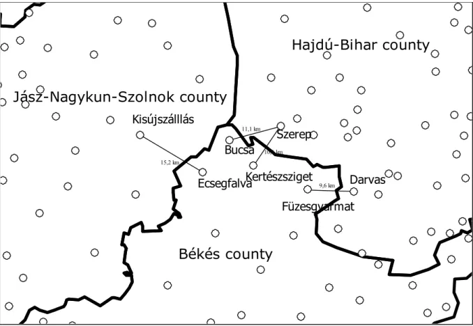
would be classified as a non-border settlement, a result that would be conceptually questionable (Figure 2).. According to the road structure, the two most peripheral settlements are “A” and “E” and both are close to the county border. “E” is at the end of a dead-end street. However, applying the road distance definition, A and E would be very far from each other and from the county border and would not be classified as a border region settlement. Combining and comparing the two distance definitions (the air distance and road network distance) would provide a sufficient, but quite complicated solution. Another possible solution, the delimitation according to the borderline of settlement, which was used by Fábián (2008), has three disadvantages in our case. Firstly, the borderline of settlements is determined mostly by historical accidents, so the location of inhabited area can be very close and very far from the administrative settlement border. Secondly, in this case, only settlements with a county borderline would be classified, without contradiction, as county border settlements. The other settlements without a borderline, which might have a centre closer to the border, would be classified as non-border region settlements. Thirdly, there are some extremely big settlements in the Hungarian Great Plain, close to the county border with their unpopulated areas, but far from their centre and inhabited area. The distance between Kisújszállás and Ecsegfalva is 15.2 kilometres, two settlements which have a common border with a county border (Figure 3).

11,1 km

10,1 km

9,6 km 15,2 km

Hajdú-Bihar county

Jász-Nagykun-Szolnok county

Békés county

Darvas

Füzesgyarmat Kertészsziget

Kisújszálllás

Ecsegfalva

Szerep Bucsa

Figure 3. Example for the border region delimitation

5,1 km - 10 km

Distance from the settlement in other county

10,1 km - 14 km -5 km

Figure 4.Settlements in border region

Table 1.The number of settlements and inhabitants in county border regions as a function of distance (2005)

Distance (km) Settlements Population

Number Proportion (%) Number Proportion (%)

5 312 9.9 366 233 3.6

6 454 14.4 620 781 6.2

7 609 19.3 882 315 8.8

8 755 23.9 2 891 386 28.7

9 894 28.3 3 333 624 33.1

10 1040 32.9 3 769 147 37.4

11 1157 36.6 4 027 689 40.0

12 1280 40.5 4 392 772 43.6

13 1398 44.3 4 678 971 46.4

14 1506 47.7 5 101 506 50.6

15 1627 51.5 5 420 644 53.8

RESULTS

The difference between border region settlements and other areas

The average personal income in settlements in border regions was compared to the following five other areas:

a) Own county average;

less than 5 km

5.1 km – 10 km

b) Average of the neighbouring settlements, which was calculated as a weighted average of every settlement inside x kilometres;

c) Average of the neighbouring settlements, but only in own county;

d) Average of the neighbouring settlements, but only in the neighbouring county; e) Neighbour county average.

The measure of dissimilarity was calculated with the following formula:







₍

₎

j

i

x

x

SS

i

x

j

x : average personal income of other area

The calculations were conducted for 14 different years. The results are very similar; therefore, for the sake of simplicity, only one year, namely 2005, will be presented. Besides the distance, the size of the settlement can play an important role; therefore, the analysis has three dimensions:

a) Type of comparison (5 different areas);

b) Distance (11 distance band categories from 5 kilometres to 15 kilometres, but the 10 kilometre one is the most important);

c) Size of settlement (4 size categories).

The calculations were made by using an own written Visual Basic Program. The settlements are more similar to their neighbourhood than to their own county average (Figure 5). However, there are interesting differences between the size categories. For larger settlements, this connection is generally not true, but for small settlements, the connection is stronger. This can be explained by the fact that, for a smaller settlement with less potential for itself, the impact of the neighbourhood is more important than for a larger settlement with a larger self-potential. This is a manifestation of the asymmetry of the neighbourhood effect. For example, it is more important to Seer Green (village with two thousand inhabitants) that London lies twenty kilometres from it, than for London that Seer Green is twenty kilometres from it. The other important factor behind the settlement size differences is that the larger settlements have larger average income also, which is closer to the county average than the lower average of smaller settlements (Table 2).

0 20 40 60 80 100 120 140 160 180 200 5 km 6 km 7 km 8 km 9 km 10 km 11 km 12 km 13 km 14 km 15 km Together above 5000 2000-5000 1000-1999 under 1000

Figure 5.The sum of difference of average personal income between the settlement and the x-kilometre neighbourhood of the

settlement/ The sum of difference of average personal income between the settlement and its own county average, %

together above 5000 2000-5000 1000-1999 under 1000 T a 2 1 u

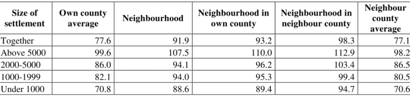
Table 2.Average personal income of county border settlements (with a 10-kilometre distance band); other areas = 100; 2005

Size of settlement

Own county

average Neighbourhood

Neighbourhood in own county

Neighbourhood in neighbour county

Neighbour county average

Together 77.6 91.9 93.2 98.3 77.1

Above 5000 99.6 107.5 110.0 112.9 98.2

2000-5000 86.0 94.1 96.2 103.4 86.5

1000-1999 82.1 94.0 95.3 99.4 80.5

Under 1000 70.8 88.6 89.4 94.7 70.6

Detailed results for the 10-kilometre distance band can be seen in Table 3. As regards the settlement size, the conclusions are the same as before. However, there are interesting differences between the various neighbourhoods: the settlements are most similar to the neighbourhood in their own county, then, in second place, is the neighbourhood, followed by the neighbourhood in different county, then the average of their own county and, at last, the average of the different county. The difference between neighbourhood in their own county and neighbourhood in different county is not big and can be explained by the larger distances between the two neighbourhoods. However, there is a striking difference between the neighbourhood and the county average. Settlements are more similar to the neighbourhood than to the average of their own county. These results show that county border effect does not exist on average.

Table 3. The sum of difference of average personal income between the settlement and the 10-kilometre neighbourhood of settlement/ The sum of difference of average personal

income between the settlement and other areas

Own county average

Neighbourhood Neighbourhood at own county

Neighbourhood at neighbour

county

Neighbour county average

Together 36032038 17377177 16322029 21111094 38253025

According to the size of settlement

Above 5000 1901021 1994463 1885104 2763174 1945236

2000-5000 2874281 2331984 1928777 3706915 3219720

1000-1999 5138042 2856031 2647229 3871097 6084164

Under 1000 26118693 10194699 9860919 10769908 27003904

Differences compared to own county average (own county=100)

Together 100 48 45 59 106

According to the size of settlement

Above 5000 100 105 99 145 102

2000-5000 100 81 67 129 112

1000-1999 100 56 52 75 118

Under 1000 100 39 38 41 103

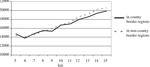
The difference of border region and non-border region settlements from their neighbourhood

difference) in border regions and, with other distances, the differences of intra-county settlements are larger (maximum 8.5%). This very small difference shows that county borders do not have an effect on the difference between the settlements and their neighbourhood. In other words, the difference between settlements and their neighbourhood is approximately the same along the county borders as along any other arbitrary or random borders.

Figure 6. Average difference between the settlements and their neighbourhood Spatial differences along the border sections

The previous analysis was whole map analysis. Spatial viewpoint was represented only in the settlement size difference and the distinction between border and non-border regions. Otherwise, the whole country was the subject of the analysis. In this part, we examine individually the county border regions. Only those borders are examined, where at least four settlements can be found. The small number of settlements by individual border regions makes the analysis by settlement size not possible.

Settlement center

Different border regions

Most different border regions Most similar border regions

Tiszaújváros effect

Danube effect Balaton effect

Figure 7.The most similar and most different border regions

10000 12000 14000 16000 18000 20000 22000

5 km 6 km 7 km 8 km 9 km 10 km 11 km 12 km 13 km 14 km 15 km

in county border regions

in non-county border regions

5 6 7 8 9 10 11 12 13 14 15 km

i

r

i

b

Vas Pest

The results support the barrier role of two natural borders, the Danube River and Lake Balaton (Figure 7). Along the Danube River, there are 43 border settlements with ten-kilometre distance. These settlements are very different from the neighbouring county averages: the sum of squares of the difference from neighbour county average is twice as from own county average, the sum of squares of the difference from neighbourhood in neighbouring county is five times more. Across the Danube River, for a 200-kilometre length between the northernmost and southernmost points, apart from Budapest, there were just two small bridges until 2002, therefore the contact between the two sides is very weak.

Large difference can be detected in East Hungary between Borsod-Abaúj-Zemplén and Hajdú -Bihar counties. Here the difference is attributable to Tiszaújváros, a small, but thanks to a big chemical factory, a very rich county border town compared to its neighbourhood. This special case of difference cannot be treated as a county border effect; it is rather an effect because of an outlier settlement.

CONCLUSIONS

According to the results, the settlements are more similar to their neighbourhood than to their county average. This similarity is decreasing with the increase of distance and the size of the settlement. This result is compliant with the first law of geography and with other results concerning the decreasing autocorrelation with increasing distance (Dusek, 2004, pp. 219-220). The special characteristics of county border regions is the smaller average settlement size and, due to the settlement size, the smaller average income.

There are only two exceptions to the general tendency: the border regions along the Danube River and along Lake Balaton. In these two cases, the natural geographical county borders do not only have a barrier effect on spatial interaction, but this barrier effect is also manifested in observable income differences on the two sides of the borders. If every county border were this type, then there would be county border effect.

The moral of the story touches upon the methodology of spatial analysis. In the analysis of spatial income differences and similar data, the counties or other middle level spatial units are often used as a basis of aggregation. The results are presented in the form of choropleth maps. This practice cannot be criticized due to practical reasons of data availability, but should always be kept in mind that space is unlike a mosaic and there are not strict, abrupt differences between the two sides of county borders. County borders may be important for administrative reasons but counties are mostly arbitrary, modifiable spatial units in the analysis of economic and social phenomena.

REFERENCES

BUJDOSÓ, Z. (2004), A megyehatár hatása a városok vonzáskörzetére Hajdú-Bihar megye példáján

[The Effect of County Border on the Catchment Area of Towns on the Example of Hajdú -Bihar County], Doktori értekezés, Debreceni Egyetem, Debrecen.

DUSEK, T. (2004), A területi elemzések alapjai[Fundamentals of Spatial Analysis], ELTE, Budapest. DUSEK, T., SZALKA, É. (2012), Is there a county border effect in spatial income differences in

Hungary?, Paper presented at the 52th Congress of the European Regional Science Association, Bratislava, Slovakia, 21-25 August 2012

FÁBIÁN, ZS. (2008), Megyehatár menti területek a Dunántúlon – erősödő vagy oldódó belső

perifériák? [Areas Along County Borders in Transdanubia – Do Internal Peripheries Become Stronger or Weaker?], Területi Statisztika, vol. 48, no. 2, pp. 164-182.

MÁRKUSNÉ ZSIBÓK, ZS. (2012), Az infláció és az árazási magatartás területi különbségei.

Nemzetközi kitekintés és magyarországi tapasztalatok [Spatial Differences in Inflation and Price-Setting Behaviour. An International Overview and Experiences in Hungary], Doktori Értekezés, Pécsi Tudományegyetem, Közgazdaságtudományi Kar.

NAGY, E. (2014), Factorial Analysis of Territorial Disparities on the Hungarian-Romanian Border Region, Romanian Review of Regional Studies, vol. 10, no. 1, pp. 7-14.

PÁSZTOR, SZ., PÉNZES, J. (2013), Altering Periphery at the Border: Measuring the Border Effect in the Hungarian-Romanian and the Hungarian-Ukrainian Border Zones, in: Horga I., Landuyt Ariane (eds.), Communicating the EU Policies Beyond the Borders, Editura Universităţii din Oradea, pp. 274-298.

PÉNZES, J. (2010), Területi jövedelmi folyamatok az Észak-alföldi régióban a rendszerváltás után

[Spatial Income Processes in the Northern Great Plain Region after the Political Transition], Studia Geographica, vol. 26, Debreceni Egyetemi Kiadó, Debrecen.

PÉNZES, J., MOLNÁR, E. (2007), Analysis of the Economical Potential in Bihor and Hajdú-Bihar Counties, in: Delanty G., Pantea D., Teperics K. (eds.), Europe from Exclusive Borders to Inclusive Frontiers, Eurolimes, vol. 4, Oradea-Debrecen, pp. 25-37.

ZSIBÓK, ZS.(2011),Az infláció területi különbségei.I. rész. [Spatial Differences in Inflation. Part I], Területi Statisztika, vol. 14 (51), no. 6, pp. 583-598.