Geosci. Model Dev., 6, 1367–1388, 2013 www.geosci-model-dev.net/6/1367/2013/ doi:10.5194/gmd-6-1367-2013
© Author(s) 2013. CC Attribution 3.0 License.
Geoscientiic
Model Development
Open Access
Geoscientiic
Mathematics of the total alkalinity–pH equation –
pathway to robust and universal solution algorithms:
the SolveSAPHE package v1.0.1
G. Munhoven
D´epartement d’Astrophysique, G´eophysique et Oc´eanographie, Universit´e de Li`ege, 4000 Li`ege, Belgium
Correspondence to:G. Munhoven ([email protected])
Received: 21 February 2013 – Published in Geosci. Model Dev. Discuss.: 12 March 2013 Revised: 17 June 2013 – Accepted: 8 July 2013 – Published: 30 August 2013
Abstract.The total alkalinity–pH equation, which relates to-tal alkalinity and pH for a given set of toto-tal concentrations of the acid–base systems that contribute to total alkalinity in a given water sample, is reviewed and its mathematical properties established. We prove that the equation function is strictly monotone and always has exactly one positive root. Different commonly used approximations are discussed and compared. An original method to derive appropriate initial values for the iterative solution of the cubic polynomial equa-tion based upon carbonate-borate-alkalinity is presented. We then review different methods that have been used to solve the total alkalinity–pH equation, with a main focus on bio-geochemical models. The shortcomings and limitations of these methods are made out and discussed. We then present two variants of a new, robust and universally convergent gorithm to solve the total alkalinity–pH equation. This al-gorithm does not require any a priori knowledge of the so-lution. SolveSAPHE (Solver Suite for Alkalinity-PH Equa-tions) provides reference implementations of several variants of the new algorithm in Fortran 90, together with new imple-mentations of other, previously published solvers. The new iterative procedure is shown to converge from any starting value to the physical solution. The extra computational cost for the convergence security is only 10–15 % compared to the fastest algorithm in our test series.
1 Introduction
Biogeochemical models have become indispensable tools to improve our understanding of the cycling of the elements in the Earth system. A central and critical component of almost all biogeochemical models is the pH calculation routine. In ocean carbon cycle models, the air–sea exchange of CO2is
directly linked to the surface ocean [CO2]; the preservation
of biogenic carbonates in the surface sediments at the sea floor is closely linked to the deep sea [CO23−] (Broecker and Peng, 1982). The fractions of CO2, HCO−3 and CO23−in the
total dissolved inorganic carbon (i.e. the speciation of the car-bonate system) are controlled by pH. Hence, pH changes in seawater may directly influence air–sea exchange of CO2or
the preservation of carbonates in the deep sea. Conversely, the dissociation of acids, such as carbonic acid, also controls pH: when the ocean takes up or releases CO2(e.g. as a
re-sult of a rise or a decline of the abundance of CO2 in the
atmosphere), its pH changes. The currently ongoing ocean acidification due to the massive release of CO2into the
at-mosphere by human activity is but one example of such an induced pH change.
The nitrogen cycle is another important biogeochemical cycle where pH plays an important role. The speciation of dissolved ammonium is – as that of any acid–base system – dependent on pH, NH3 being more abundant than NH−4 at
The realistic modelling of biologically mediated fluxes (e.g. marine primary or export production) requires the co-limitation or even inhibition by different chemical compo-nents to be taken into account. The nitrogen and carbon cy-cles, already mentioned above, strongly interact, both in the ocean and on land. In the ocean, Fe and other metals act as micronutrients and once again, pH plays an important role as the solubility of metals is strongly dependent on pH (Millero et al., 2009). The resulting coupling of the biogeochemical cycles of different elements makes biogeochemical models become more and more complex and pH calculation more and more difficult.
Biogeochemical models are now increasingly used for set-tings that are strongly different from present day. Typical ap-plications include future ocean acidification (e.g. Caldeira and Wickett, 2003), the Paleocene–Eocene Thermal Max-imum (e.g. Ridgwell and Schmidt, 2010), Snowball Earth (e.g. Le Hir et al., 2009), etc. Some commonly used pH solvers may possibly become unstable and produce unreli-able results. The convergence properties of currently used so-lution methods has actually never been systematically tested. Unfortunately, information on pH solver failures is only seldom published. Zeebe (2012) reports for his LOSCAR model that negative H+ concentrations may be obtained when starting with total alkalinity and dissolved inorganic carbon concentrations in a very high ratio, requiring the model run to be restarted with the respective concentrations in a lower ratio. Hofmann et al. (2010) also indicate that the standard pH solving routine in their R modelling environ-ment AquaEnv may fail when trying to calculate the pH for samples with very low or zero dissolved inorganic carbon concentrations. In this case, they resort to a general purpose interval based root finding routine instead, adopting a very large bracketing interval (see Hofmann et al., 2012), possibly leading to a considerable performance loss. Andy Ridgwell, in his editorial comment to the companion discussion paper, mentions convergence problems encountered with the GE-NIE model code (Ridgwell et al., 2007) encountered while studying the effect of an artificial addition of lime (CaO) to the ocean surface (a particular geoengineering method meant to accelerate the uptake of carbon dioxide from the atmo-sphere) once total alkalinity came to exceed the typical sur-face ocean concentrations of dissolved inorganic carbon by about a factor of two. As we will show below, the three mod-els use essentially equivalent pH calculation methods, which become divergent under those typical conditions.
The speciation of any acid system, i.e. the determination of the concentrations of each one of the undissociated and the different dissociated forms of an acid, is an underdeter-mined problem if only the total concentration and thermody-namic or stoichiometric constants are known. This underde-termination can be lifted if pH is known. Being dependent on temperature and pressure, neither pH nor [H+] are, how-ever, well suitable for being used in transport equations, and thus in biogeochemical models. In biogeochemical models,
the common way to resolve this underdetermination is to consider another conservative quantity: total alkalinity, also called titration alkalinity. Total alkalinity, which is also an experimentally measurable quantity, ties all the different acid systems present in a water sample together and allows us to solve the speciation problem. In comparison to pH, it has the advantage of being a conservative quantity: it is only con-trolled by its sources and sinks, and it is independent on tem-perature and pressure (Zeebe and Wolf-Gladrow, 2001).
In the following section, we provide a comprehensive in-troduction to the concept of alkalinity. In our exploration of the mathematical properties of the equation that relates [H+]
to total alkalinity start with a detailed presentation of various approximations commonly used for present-day seawater. The analysis of the mathematical properties of these approx-imations will provide useful hints for the characteristics of the general case. In Sect. 3 of this paper, we present solution methods for deriving pH from each of the various approx-imations to total alkalinity considered. Complications that might possibly arise from the various pH scales that are in use in marine chemistry are elucidated in Sect. 4. In Sect. 5, we then show that there are intrinsic bounds that bracket the root of the total alkalinity–pH equation, and that can be di-rectly derived from the approximation used to represent total alkalinity. The existence of such bounds makes it possible to define a new, universal algorithm to solve the alkalinity–pH equation, which requires no a priori knowledge of the root. A reference implementation of two variants of the new algo-rithm is presented in Sect. 6. The algoalgo-rithms are tested for their efficiency and robustness and their performance com-pared with that of the most common previously published general solution methods.
2 Total alkalinity: general definition and approximations
In the following parts of this section, we review a number of aspects of total alkalinity in natural waters. The main focus will be put onto seawater and on the carbonate system, but all the presented developments can be applied to any natu-ral water sample, provided the required thermodynamic con-stants are known. We briefly recall the different approxima-tions commonly used for calculating pH and the speciation of acid systems. We will then establish a few basic proper-ties of the expressions that relate the various types of alka-linity to total concentrations and pH. Although simple, these properties do not seem to have been previously explored in detail, nor exploited for designing methods of solution of the alkalinity–pH equation.
2.1 Total alkalinity
2.1.1 General definition
Total alkalinity, also called titration alkalinity, denoted here AlkT, reflects the excess of chemical bases of the solution
rel-ative to an arbitrary specified zero level of protons, or equiva-lence point. Ideally, AlkTrepresents the amount of bases
con-tained in a sample of seawater that will accept a proton when the sample is titrated with a strong acid (e.g. hydrochloric acid) to the carbonic acid endpoint. That endpoint is located at the pH below which H+ions get more abundant in solution
than HCO−3 ions; its value is close to 4.5. H+added to water
at this pH by adding strong acid will remain as such in solu-tion. Please notice that, for the sake of a simpler notation, we follow here the common usage of denoting protons in solu-tion by H+, although free H+ions sensu stricto do only exist in insignificantly small amounts in aqueous solutions. Each proton is rather bound to a water molecule to form an H3O+
ion, and each of these H3O+in turn is furthermore generally
hydrogen bonded to three other H2O molecules to form an
H9O+4 ion (Dickson, 1984).
Rigorously speaking, AlkT is defined as the number of
moles of H+ions equivalent to the excess of “proton accep-tors”, i.e. bases formed from acids characterized by apKA≥
4.5 in a solution of zero ionic strength at 25◦C, over “proton
donors”, i.e. acids withpKA<4.5 under the same
condi-tions, per kilogram of sample (Dickson, 1981).
With emphasis on the most important contributors, a rather complete expression for AlkTin a seawater sample is
AlkT= [HCO−3] +2× [CO32−] + [B(OH)−4] + [OH−]
+ [HPO24−] +2× [PO43−] + [H3SiO−4]
+ [NH3] + [HS−] +2× [S2−] +. . .
− [H+]f−[HSO−4]−[HF]−[H3PO4]−. . . , (1)
where the ellipses refer to other potential proton donors and acceptors generally present at negligible concentrations only. All of the concentrations are total concentrations (which in-clude free, hydrated and complexed forms of the individ-ual species), except for[H+]f, which only includes the free
and hydrated forms. There are alternative definitions that can be found in the literature, which lead to similar, although not necessarily exactly the same, expressions. However, the above definition is the one that reflects the titration proce-dure used to measure alkalinity the most accurately. We will therefore base the following developments upon it.
In other natural water samples (lake, river, or brines) the constituent list in Eq. (1) needs to be adapted: some con-stituents may be neglected and bases of other acid sys-tems have to be included (e.g. bases derived from organic acids, from dissolved metals, etc.). While total alkalinity in seawater samples typically ranges between about 2 and 2.6 meq kg−1, acid mine drainage samples may even present negative alkalinity, representing the fact that a strong base
instead of a strong acid must be added to reach the equiv-alence pH point of 4.5. Interested readers may refer, e.g. to Kirby and Cravotta III (2005) and references therein for such – from a marine chemist’s point of view – exotic samples. 2.1.2 The pH–total alkalinity equation
Total alkalinity as defined above is a conservative quantity with respect to mixing, changes in temperature and pressure (Wolf-Gladrow et al., 2007). It is therefore a cornerstone in biogeochemical cycle models which are most conveniently formulated on the basis of conservation equations. In such models, definition/Eq. (1) above, or an adequate variant, is used to solve the inverse problem for [H+]. All of the in-dividual species concentrations appearing in Eq. (1) can be expressed in terms of the total concentrations of the acid sys-tems that they respectively belong to and of[H+]. Given the evolutions of the total concentrations of all the acid systems considered (dissociated and non-dissociated forms) and of AlkT– all of which can be derived from appropriate
conser-vation equations – expression (1) is interpreted as an equa-tion for[H+]or, equivalently, pH. We will therefore call that equation the total alkalinity–pH equation.
We might actually have called our equation simply the pH equation. AlkTdoes indeed not play any special or more
im-portant role than any of the total concentrations of the other acid systems considered. We do, however, feel that this name would have been too general and thus prefer to include “total alkalinity” in the name to reflect that the overall structure of the equation derives from the definition of total alkalinity. 2.1.3 Typical applications in biogeochemical models
In a typical global ocean carbon cycle model, total alkalinity may commonly be approximated by
AlkT≃ [HCO−3] +2× [CO
2−
3 ] + [B(OH)−4] + [OH−]−[H+], (2)
where[H+] ≃ [H+]f+ [HSO4−+ [HF]. [HCO−3] and [CO23−]
can be expressed as a function of the total concentration of dissolved inorganic carbon,CT, and [H+] (see Sect. 2.2.1 for
details) while [B(OH)−4] can be expressed as a function of the total borate concentration,BT, and [H+] (see Sect. 2.2.2
for details); [OH−] is directly linked to [H+] via the
equi-librium constant for the dissociation of water. Accordingly, Eq. (2) provides a relationship between CT,BT, AlkT and
[H+] (i.e. pH). The model provides conservation equations
forCTand AlkT;BTcan generally be taken proportional to
salinity, whose evolution either follows a prescribed scenario or may also derived from a conservation equation. Relation-ship (2) thus reduces to an equation in [H+]. The solution of that equation finally provides a means to calculate the com-plete speciation of the carbonate and the borate systems.
of the individual species concentrations that need to be con-sidered in Eq. (1) for that particular application is expressed in terms of the total concentration of the acid system that it belongs to and conservation equations, scenarios or measure-ments that are used to evaluate all of the total concentrations, including total alkalinity. These steps again reduce Eq. (1) into an equation in [H+], whose solution provides a direct means to calculate the speciations of all the systems consid-ered.
2.2 Common approximations for total alkalinity in seawater
Here we first analyse the forward problem for a few spe-cific approximations used for seawater: for given total con-centrations of dissolved inorganic carbon, total borate, etc., we analyse how the expressions for the different types of al-kalinity change as a function of[H+]. This simple analysis
will already provide valuable insight into the overall math-ematical properties of the total alkalinity–pH equation and its subcomponents, which we can exploit later for the most general case.
2.2.1 Carbonate alkalinity
The contribution of the carbonic acid system (or carbonate system) to total alkalinity is called carbonate alkalinity and we denote it by AlkC:
AlkC= [HCO−3] +2[CO23−].
Upon substitution of the concentrations of the species by their fractional expressions as a function of[H+],
[HCO−3] =CT
K1[H+]
[H+]2+K
1[H+] +K1K2
and
[CO23−] =CT
K1K2
[H+]2+K
1[H+] +K1K2 ,
whereCT is the total concentration of dissolved inorganic
carbon (CT= [CO2] + [HCO−3] + [CO 2−
3 ]),K1 andK2 are
the first and second dissociation constant for carbonic acid, we get
AlkC=CT
K1[H+] +2K1K2
[H+]2+K
1[H+] +K1K2 .
For constantCT, the right-hand side is a strictly decreasing
function of[H+]: its derivative with respect to[H+]is strictly negative for positive[H+]. As a consequence, 0<AlkC<
2CT ifCT6=0. Both bounds are strict (i.e. they cannot be
reached) and represent the limits of AlkC(CT; [H+]) for
[H+] → +∞(lower bound) and [H+] →0 (upper bound), forCTfixed.
2.2.2 Carbonate and borate alkalinity
The second most important component of natural present-day seawater alkalinity is borate alkalinity, AlkB. Together
with the carbonate alkalinity we have AlkCB=AlkC+AlkB= [HCO−3] +2[CO
2−
3 ] + [B(OH)−4].
Upon substitution of the individual species concentrations by their fractional expressions as a function of[H+], we get
AlkCB=CT
K1[H+] +2K1K2
[H+]2+K
1[H+] +K1K2+ BT
KB
[H+] +KB,
whereBTis the total concentration of dissolved borates and KBis the dissociation constant for boric acid. For constant BT, AlkBis again a strictly decreasing function with[H+],
similarly to AlkC. Hence, for constant CT andBT, AlkCB
is a strictly decreasing function with[H+]and, as a
conse-quence, 0<AlkCB<2CT+BTas long asCT+BT6=0.
2.2.3 Carbonate, borate and water self-ionization alkalinity
In a third stage, we may consider the alkalinity that arises from the dissociation of the solvent water itself (by self-ionization) in addition to carbonate and borate alkalin-ity and get the next important approximation for natural present-day seawater, called practical alkalinity by Zeebe and Wolf-Gladrow (2001):
AlkCBW
=AlkCB+ [OH−]−[H−]
= [HCO−3] +2[CO23−] + [B(OH)−4] + [OH−]−[H+].
Upon substitution by the respective speciation relationships, we get
AlkCBW=CT
K1[H+] +2K1K2
[H+]2+K
1[H+] +K1K2
+BT KB
[H+] +KB+ KW
[H+]− [H+],
(3)
whereKWis the dissociation constant of water in seawater.
At this stage, we do not want to insist on subtleties related to pH scales. Normally, the last term[H+]in the two previous equations should actually read[H+]f. We will address the
difference between [H+] and[H+]fin Sect. 4 below.
Since AlkCBis decreasing with[H+], for constantCTand BT, the same holds for AlkCBW, becauseKW/[H+]−[H+]
is again decreasing with [H+]. However, unlike AlkCB,
AlkCBW is unbounded and it can take arbitrarily low values
2.2.4 Contribution of a generic acid system to total alkalinity
In common seawater, AlkCBWis entirely sufficient even for
applications that require high accuracy. However, in some cases other systems than the carbonate and borate systems need to be considered. This is especially the case in suboxic and anoxic waters, such as semi-closed fjords (e.g. Fram-varen Fjord in Norway studied by Yao and Millero, 1995) or at a larger scale, the Black Sea (e.g. Dyrssen, 1999), where, e.g. the contribution from sulphides cannot be neglected.
In order to generalize our analysis of the total alkalinity– pH equation, let us consider a generic acid, denoted by HnA, that may potentially lead tonsuccessive dissociation reac-tions, characterized by stoichiometric dissociation constants
K1, K2, . . ., Kn, respectively:
HnA⇋H++Hn−1A−, K1=[H +][H
n−1A−]
[HnA]
Hn−1A−⇋H++Hn−2A2−, K2=[H +][H
n−2A2−]
[Hn−1A−] ..
. ...
HA(n−1)−⇋H++An−, Kn= [H
+][An−]
[HA(n−1)−].
For simplicity, we omit the “∗” superscript commonly used elsewhere to differentiate stoichiometric from thermody-namic dissociation constants (i.e. elsewhere stoichiometric constants generally writeKi∗instead ofKi). Throughout this paper, the constants used will relate concentrations and not activities. As such, they include the effect of activity coef-ficients that differ from unity. The values of such constants not only depend on temperature and pressure but also on the ionic strength of the solution. Everything developed here furthermore applies to all kinds of acids, be they of Arrhe-nius, Brønsted–Lowry, Lewis or any other type, even if the adopted notation could possibly suggest that our develop-ments only apply to Arrhenius-type acids.
If we denote the total concentration of dissolved acid HnA by [6A]=[HnA] +. . .+ [An−], the fractions of undissoci-ated acid and of the various dissociundissoci-ated forms Hn−1A−,
Hn−2A2−, . . . , An−are
[HnA]
[6A] =
[H+]n
[H+]n+K
1[H+]n−1+K1K2[H+]n−2
+...+K1K2···Kn
= [H
+]n
[H+]n+Pn
j=1[
H+]n−j j
Q
i=1 Ki
,
[Hn−1A−]
[6A] =
K1[H+]n−1
[H+]n+Pn
j=1[
H+]n−j j
Q
i=1 Ki
,
.. .
[Hn−jAj−]
[6A] =
( j
Q
i=1
Ki)[H+]n−j
[H+]n+Pn
k=1[
H+]n−kQk
i=1 Ki
,
.. .
[An−] [6A] =
n
Q
i=1 Ki
[H+]n+Pn
j=1[
H+]n−j j
Q
i=1 Ki
.
The joint contribution of all the different dissociated and non-dissociated forms of HnA to alkalinity, proton donors and proton acceptors alike, is then equal to
AlkA= n
X
j=0
(j−m)[Hn−jAj−],
wheremis an integer constant, which is dependant on the so-called zero proton level of the system under consideration:
– mis such thatpKm<4.5< pKm+1 if pK1<4.5
andpKn>4.5 – m=0 ifpK1>4.5
– m=nifpKn<4.5
Since pKm<4.5, all of the Hn−jAj− in the HnA . . . -An−system forj=0, . . ., m−1 are proton donors: the last one (j=m−1) has a strength of 1 eq mol−1, the second to last one (j=m−2) of 2 eq mol−1, etc. SincepKm+1>4.5,
the dissociation products Hn−jAj−forj=m+1, . . ., nare proton acceptors, the first one (j=m+1) with a strength of 1 eq mol−1, the second one (j =m+2) with a strength of 2 eq mol−1, etc. For the carbonic acid system, e.g.n=2 and
From the previous expressions for the species fractions, we then find that
AlkA([H+])= [6A] n
P
j=0
(j−m)5j[H+]n−j n
P
j=0
5j[H+]n−j
= [6A]
n
P
j=0
j 5j[H+]n−j n
P
j=0
5j[H+]n−j
−m
, (4)
where we have defined
5j= j
Y
i=1
Ki, j =1, . . ., n and 50=1 (5)
to simplify the notation.
Similar to the carbonate and borate systems above, AlkAis
strictly decreasing with[H+], for[6A]fixed. A mathemati-cally rigorous demonstration of this behaviour for the general case is provided in Appendix A.
There are two corollaries of this monotonic behaviour worth emphasizing.
1. For any acid system HnA-. . . -An−, AlkAis bounded: it
has a supremum which is equal to(n−m)[6A](i.e. the limit for[H+] →0, not actually reachable though), and an infimum, which is equal to−m[6A](i.e. its limit for[H+] → +∞, also not actually reachable); both of
these could, theoretically, be negative ifmis sufficiently large.
2. For a water sample that contains a set of acids HniA[i],
(i=1, . . .) of respective known total concentrations
[6A[i]]and with zero proton levels respectively
char-acterized bymi, the total alkalinity–pH equation,
X
i
AlkA[i]([H+])+
Kw
[H+]−[H+]f−AlkT=0, (6)
has exactly one positive root[H+], for any given value
of AlkT: the sum of the respective alkalinity
contribu-tions over the set{HniA[i]|i=1, . . .}of all the acid sys-tems active in the sample is a strictly decreasing func-tion of [H+]; the contribution from the dissociation of water is also strictly decreasing with [H+], and may the-oretically take any value between+∞and−∞.
3 Alkalinity–pH equation in biogeochemical models: approximations and methods of solution
In this section, we are going to review the most common ap-proximations used in ocean carbon and biogeochemical cy-cle models, focusing on how the corresponding equation is solved.
3.1 Carbonate alkalinity based solutions
The straight approximation AlkT≃AlkC is often used in
textbooks (e.g. Broecker and Peng, 1982). There are only a few models (e.g. Opdyke and Walker, 1992; Walker and Opdyke, 1995) that use it directly for their carbonate chem-istry speciation. For numerical modelling purposes, its us-age is indeed somewhat problematic. [H+] calculated from AlkT andCTdata, by assuming that AlkC=AlkT are
typi-cally 30–40 % too low (i.e. 0.15–0.2 pH units too high) for present-day seawater samples. Furthermore, the sensitivity of theCT-AlkCsystem to perturbations is stronger than that of
theCT-AlkCBWsystem: equilibriumpCO2changes, e.g. are
of the order of 20 % larger (Munhoven, 1997).
The calculation of [H+] fromCT-AlkCremains
neverthe-less important, as more advanced methods such as those pro-posed by Bacastow (1981), Peng et al. (1987) or Follows et al. (2006), where AlkC is iteratively recalculated from
more complete approximations to AlkT(ICAC methods – see
below), rely on it.
3.1.1 Fundamental solution
For given AlkCandCT (CT>0), the equation to solve for
[H+]is
RC([H+])≡CT
K1[H+] +2K1K2
[H+]2
+K1[H+] +K1K2−
AlkC=0. (7)
Following our discussion in Sect. 2.2.1, Eq. (7) has a positive root if and only if 0<AlkC<2CT; if there is a positive root,
it is unique.
Equation (7) can be directly solved after conversion to the quadratic equation:
PC([H+])≡ [H+]2+a1[H+] +a0=0, (8)
where
a1=K1
1− CT
AlkC
and a0=K1K2
1− 2CT
AlkC
.
For valid AlkC values (i.e. for 0<AlkC<2CT), this
quadratic equation has two real roots, a positive and a nega-tive one. The posinega-tive root is
[H+]=Q(AlkC, CT)≡ K1
2
C
T
AlkC−
1+p1C
, (9)
where
1C=
1− CT
AlkC
2
+4K2
K1
2CT
AlkC−
1
. (10)
For AlkCvalues that are out of range Eq. (8) either has two
3.1.2 Alternative methods
There are other methods to derive[H+]from AlkCandCT.
All of them ultimately seem to rely on the formulae of Park (1969) for deriving the complete speciation of the carbon-ate system directly from AlkCandCT, without explicitly
us-ing [H+]. Antoine and Morel (1995) first calculate [CO2]
from CT and AlkC (which involves the solution of a first
parabolic equation), and then derive [H+] from the relation-ship[CO2]=AlkC[H+]2/(K1[H+]+2K1K2), which requires
the solution of a second parabolic equation. Ridgwell (2001) first determines the complete speciation of the carbonate sys-tem, referring for the adopted procedure to Millero and Sohn (1992), who actually only report the formulae of Park (1969). He then derives two different estimates for [H+], based upon
the definitions of the first and second dissociation constants of carbonic acid, and finally uses the geometric mean of these two estimates as a solution for Eq. (7).
There are no obvious advantages for calling upon these methods instead of the direct quadratic solution above. Even if carefully implemented, both require a significantly higher number of operations than the solution outlined above. Those methods offer a direct access to carbonate speciation (at least in part), which can, however, also be calculated at little extra cost from [H+].
3.1.3 Iterative carbonate alkalinity correction methods
In most common natural settings, the difference between AlkC and AlkT, albeit small, leads to significant errors on
[H+], if AlkTis used in place of AlkCand one of the
proce-dures above is used to calculate it fromCT. To overcome this
problem, AlkCcan be estimated from AlkT, and then
itera-tively corrected until stabilization occurs. Such a procedure, which we call here iterative carbonate alkalinity correction (ICAC) can a priori be used with arbitrary chemical com-positions, provided AlkCrepresents a significant fraction of
AlkT. If AlkC makes up only a small fraction of AlkT, the
method is likely to exhibit unstable behaviour.
In the most straightforward ICAC method, one starts from a trial valueH0for [H+], a first estimate AlkC,0is obtained
by subtracting the concentrations of all non-carbonate com-ponents from AlkT. That AlkC,0 is then used to calculate
a new (improved) estimateH1for [H+] from Eqs. (9) and
(10) or one of the alternative methods. H1 is then used to
calculate a new estimate AlkC,1from AlkTas above and the
procedure is iterated until some predefined convergence cri-terion is fulfilled. This procedure is a classical fixed-point iteration:
Hn+1=Q(AlkC(AlkT, Hn), CT). (11)
In this recurrence, AlkC(AlkT, Hn)is the estimate of AlkC
obtained from AlkT by subtracting all the non-carbonate
components estimated by usingHn. Pure fixed-point itera-tive schemes may be prone to convergence problems (slow
convergence or no convergence at all). If the procedure is convergent, the rate of convergence is linear.
This plain fixed-point-iteration ICAC method was recently made popular again by Follows et al. (2006). These authors argue that in carbon cycle model simulation experiments, where there is little change in pH from one time step to the next, a single iteration may already provide a sufficiently accurate estimate of [H+] to derive acceptablepCO2
esti-mates, for any chosen approximation of total alkalinity. Fol-lows et al. (2006) suggest, if necessary, to repeat the fixed-point iteration until a sufficiently accurate estimate is found. There are a number of models that rely on the ICAC ap-proach for their pH determination. Peng et al. (1987) con-sider AlkCBW plus the contributions from silicic and
phos-phoric acid systems in their representation of total alkalin-ity.1They use an initial value of 10−8and stop their iterations
once|(1H )/H|<0.005 %. They report that less than ten it-erations are generally sufficient. Antoine and Morel (1995) adopt AlkCBW as an approximation to AlkT. At each step,
they derive [H+] from CT and AlkC by using their special
procedure described above. They iterate until two succes-sive AlkCestimates differ by less than 10−8(no units given).
Ridgwell (2001) adopts AlkCB+ [OH−] +1.1[PO34−]as an
approximation to total alkalinity. He calculates [H+] at each step fromCTand AlkCby using his own procedure described
above. GENIE (Ridgwell et al., 2007) initially used the same procedure as Ridgwell (2001); in more recent versions of GENIE, a complete representation of the phosphoric acid component is used (A. Ridgwell, personal communication, 2012). Arndt et al. (2011) use AlkCBW+ [HS−] as an
ap-proximation to total alkalinity in GEOCLIMreloaded. They continue to iterate until|AlkCBW+[HS−]−AlkT|<10−6(no
units given). The method is further used in LOVECLIM (A. Mouchet, personal communication, 2012) with AlkCBW
as an approximation for total alkalinity (Goosse et al., 2010) and most probably still in some others that, unfortunately, do not provide details about the calculation procedures adopted. Bacastow (1981) proposed a variant to improve the rate of convergence of fixed-point iterations. That variant only uses the recurrence described above for the first two iterates. From the third iteration on, Bacastow (1981) switches to a secant method to solve the fixed-point equation H− Q(AlkC(AlkT, H ))=0.2Fixed-point iterations are thus only
used to provide starting values for the solution of the fixed-point equation by the secant method. The rate of convergence of the method is strongly increased by this approach (and the
1Peng et al. (1987) adopt, however, a slightly different
defini-tion of total alkalinity by systematically weighting species by their respective charge. This leads to differences with the phosphoric acid system: e.g. the definition of Peng et al. (1987) is equivalent to adoptingm=0 for the phosphoric acid system.
2Bacastow (1981) actually solves the alkalinity equation for the
domain of convergence slightly enlarged – see numerical ex-periments below). However, for someCT-AlkTcombinations
the underlying fixed-point equation may still give rise to con-vergence problems, even with the secant method. However as will be shown below, the method of Bacastow (1981) is strongly preferable over the pure fixed-point scheme.
The Hadley Centre Ocean Carbon Cycle (HadOCC) model (Palmer and Totterdell, 2001) uses Bacastow’s method for its carbonate speciation calculation, with the AlkCBW
approxi-mation.
3.2 Carbonate and borate alkalinity based solution
Only a few models appear to use pH calculation rou-tines based upon AlkCB. MBM-MEDUSA (Munhoven and
Franc¸ois, 1996; Munhoven, 1997, 2007) is one of them, the model of Marchal et al. (1998) is another one.
3.2.1 Basic formulation and solution methods
The equation to solve for[H+]is, for given AlkCB,CT and BT,
RCB([H+])≡CT
K1[H+] +2K1K2
[H+]2+K
1[H+] +K1K2
+BT KB
[H+] +KB−AlkCB
=0. (12)
This equation may be converted into the polynomial equa-tion:
PCB [H+]≡ [H+]3+c2[H+]2+c1[H+] +c0=0, (13)
with
c2=KB
1− BT
AlkCB
+K1
1− CT
AlkCB
,
c1=K1
KB
1− BT
AlkCB− CT
AlkCB
+K2
1−2 CT AlkCB
,
c0=K1K2KB 1−
2CT+BT
AlkCB
.
Following our discussion in Sect. 2.2.2, Eq. (12) has a pos-itive root if and only if 0<AlkCB<2CT+BT; if there is
a positive root, it is unique. The same holds for the cubic Eq. (13).
The cubic equation could possibly be solved with closed formulae, such as Cardano’s formulae (which may, however, suffer from precision problems, require numerically expen-sive cubic root evaluations or possibly complex arithmetic) or Vi`ete’s trigonometric formulae (which require a combi-nation of an arccosine, a cosine and a square root). When adopted, the cubic Eq. (13) is therefore generally solved nu-merically with a Newton–Raphson scheme. In this case, de-termining an adequate starting value is the main problem to address in order to design a robust and fast solution algo-rithm.
3.2.2 Efficient starting value for iterative methods
An excellent initial value for the Newton–Raphson scheme can be found by adopting the following procedure:
1. locate the local minimum closest to the largest root – if it exists, it is the extremum;
2. develop PCB([H+])to second order around that
mini-mum; and
3. determine the greatest root of the resulting parabola and use it as a starting value.
That local minimum, if it exists (i.e. ifc22−3c1>0), is
lo-cated at
Hmin=
−c2+
q
c22−3c1
3 =
−c1 c2+
q c22−3c1
.
The Taylor expansion to second order inHmin, thus intersects
theHaxis on the right-hand side ofHminat
H0=Hmin+
v u u
t−
PCB(Hmin)
q c22−3c1
,
providedPCB(Hmin) <0. By completing the Taylor
expan-sion to third order, it is straightforward to show thatH0is
greater than the root.
The so-definedH0provides an excellent starting value not
only for solving the cubic polynomial equation, but also for other iterative methods.
3.3 Carbonate, borate and water self-ionization alkalinity
With AlkCBW,CTandBTgiven, the equation to solve is RCBW([H+])
≡CT
K1[H+] +2K1K2
[H+]2+K
1[H+] +K1K2+ BT
KB
[H+] +KB
+ KW
[H+]− [H+]−AlkCBW=0. (14)
One may either solve this equation in that rational fraction form with some iterative root-finding method or by one of the ICAC methods described above, or one may transform it into a quintic polynomial equation:
PCBW([H+])
≡ [H+]5+q4[H+]4+q3[H+]3+q2[H+]2+q1[H+]+q0
=0
with
q4=AlkCBW+K1+KB, q3=(AlkCBW−CT+KB)K1
+(AlkCBW−BT)KB+K1K2−KW, q2=(AlkCBW−2CT+KB)K1K2
+(AlkCBW−CT−BT)K1KB−K1KW−KBKW, q1=(AlkCBW−2CT−BT)K1K2KB
−K1K2KW−K1KBKW, q0= −K1K2KBKW.
The polynomial equation can then be solved with appropriate standard root finding techniques, selecting the positive root found. Equations (15) and (14) have the same unique positive root: when Eq. (14) is multiplied by the product of all the denominators of the fractions included – a product that does not change sign for[H+]>0 – to transform it into Eq. (15) no new sign changes can be obtained for[H+]>0.
AlkCBWis probably the most commonly used
approxima-tion for total alkalinity in global carbon cycle models of all kinds of complexity. It was already adopted by Bacastow and Keeling (1973), who based their pH calculation on the quintic Eq. (15), which they solve by Newton’s method, with a stopping criterion|(1H )/H|<10−10. Hoffert et al. (1979) adopt the same procedure (for which they refer to Keeling, 1973 and Bacastow and Keeling, 1973), but with a less strin-gent stopping criterion |(1H )/H|<10−6. Keeling (1973)
uses a variant, whereCTis replaced by an equivalent term in pCO2.
As already mentioned above, LOVECLIM (Goosse et al., 2010) and HadOCC (Palmer and Totterdell, 2001) use AlkCBWas an approximation for total alkalinity. AlkCBWis
also used in the PISCES model (Aumont and Bopp, 2006), following a simplified version of the OCMIP standard proto-col (see next section). PISCES is included in NEMO and in some versions of the Bern3D model (Gangstø et al., 2011). Other models that base their pH calculation on AlkCBW
include the Hamburg Model of the Ocean Carbon Cycle (HaMOCC) family (Maier-Reimer and Hasselmann, 1987; Heinze et al., 1991; Maier-Reimer, 1993; Maier-Reimer et al., 2005), the models of Bolin et al. (1983) and Shaffer et al. (2008). No details regarding the adopted solution algo-rithms are provided, though.
3.4 More complete approximations: rational function based solvers
When additional components in total alkalinity need to be considered besides carbonate, borate and water self-ionization, converting the resulting rational function equa-tion to an equivalent polynomial form becomes more and more tedious and the rational function form becomes the pre-ferred basis for finding the solution. ICAC methods are the only ones that we have encountered so far that could
pos-sibly be used to address this problem. However, they bear some potential pitfalls: despite having a solution, the under-lying fixed-point equation may be difficult to solve numeri-cally; intermediate estimates of AlkCmay go out of bounds
(remember that AlkC may only take values between 0 and
2CT). ICAC methods can therefore not be guaranteed to find
the solution.
The only commonly used carbonate chemistry routine that directly solves the rational function form of the equation is that from the Ocean Carbon Cycle Model Intercompari-son Project (OCMIP). For the purpose of that project, Orr et al. (2000) prepared standard carbonate speciation rou-tines. Total alkalinity is approximated by AlkT≃ [HCO−3] +
2×[CO23−]+[B(OH)−4]+[OH−]+[HPO2−
4 ]+2×[PO 3− 4 ]+
[H3SiO−4]−[H+]f−[HSO−4]−[HF]−[H3PO4].The different
species concentrations were, as above, expressed as a func-tion of the total concentrafunc-tions of their respective acid sys-tems and of [H+]. The resulting equation was then solved for pH by a hybrid Newton-bisection method, based upon the rtsafesolver from Press et al. (1989). All of the models that participated in OCMIP had to use the provided routines for a set of well defined experiments. A number of models still routinely use these OCMIP routines for their pH calcu-lations. These include some versions of the Bern3D model (M¨uller et al., 2008) and the NCAR global coupled carbon cycle–climate model CSM1.4-carbon (Doney et al., 2006). As mentioned above, PISCES (Aumont and Bopp, 2006) includes a version of the OCMIP solver trimmed down to AlkCBWonly. Other models still offer the OCMIP solvers as
an option.
3.5 Other approaches
Luff et al. (2001) have provided a suite of pH calculation routines mainly meant to be used in reactive transport mod-els, but suitable for general speciation calculations as well. The methods proposed by Luff et al. (2001) solve the com-plete system of equations that control the chemical equilibria between the individual species considered in the total alka-linity approximation. These are required for grid-based re-active transport models where different species are diffusing at different diffusivities. For common applications in biogeo-chemical carbon cycle models, this approach is nevertheless unnecessarily complex.
environment they were designed for. As their names already suggest, they are mainly aimed at carbonate speciation cal-culations. They also often offer the possibility to chose any two among pH, [CO2] (orpCO2), [HCO−3], [CO
2−
2 ],CT, or
AlkTto calculate all the others.
4 pH-scale considerations
As shortly mentioned above, there are a few subtleties related to pH scales that still need to be clarified. The mere existence of more than one pH scale reflects the difficulties to apply the fundamental definition of pH (which involves an immeasur-able quantity – see next section) to the experimental determi-nation of acidity in seawater. All of our calculations never-theless rely on the availability of equilibrium constants that have to be experimentally derived and we therefore have to care about differences arising from the usage of various pH scales.
Let us, similarly to Bates and Culberson (1977) consider the equilibrium relationship (the mass action law) for an acid dissociation reaction. Without loss of generality, we may write that relationship for the first dissociation reaction of our generic acid from Sect. 2.2.4:
K1=[
H+][Hn −1A−]
[HnA] .
When the dependency ofK1 on temperature and salinity is
experimentally determined, the fraction[Hn−1A−]/[HnA]is measured or calculated for each experiment. [H+] cannot be
directly measured, but gets assigned a value from some pH measurement via the reverse relationship[H+]=10−pH. Tak-ing the negative logarithm (antilogarithm) of the previous equation and writingpK1= −logK1, we get
pK1=pH−log
[Hn−1A−]
[HnA]
.
In a given setting (i.e. for given temperature, salinity, pres-sure, solution chemistry, etc.), the ratio[Hn−1A−]/[HnA]is set and different calibrations of the pH-meter used, i.e. ferent scales chosen for the pH-meter, will thus produce dif-ferentpK1values. Any experimentally derived
parameteri-zation forK1can therefore only be used in conjunction with
a H+concentration scale that is consistent with the pH scale
that was used to derive it. Before a particular empirical pa-rameterization forK1can be used with a different scale of pH
(e.g. due to a different conventional or operational definition of pH), it must be converted.
Additional conversion may be required because of the usage of different concentration units: both mo-lal units (mol/kg-H2O) and mol/kg-seawater are
com-mon. They can be converted according to[mol/kg-SW] =
m(mol/kg-H2O)×(1−0.001005S) (Dickson et al., 2007,
chapter 5, p. 13), whereS denotes salinity. ForS=35, the
difference between the values is about±3.5%; in log units, the values differ by±0.016.
There is abundant literature on pH scales for seawater. Besides the original fundamental papers by, e.g. Hansson (1973), Bates and Culberson (1977), Khoo et al. (1977), Dickson and Riley (1979), Bates (1982) or Dickson (1990), the classical review papers by Dickson (1984, 1993), or stan-dard textbooks (e.g. Zeebe and Wolf-Gladrow, 2001), there are also several recent papers on the subject, such as the views by Dickson (2010) and Marion et al. (2011) or the re-search paper by Waters and Millero (2013). In the following sections, we will therefore only give a comparatively general overview, which we have nevertheless tried to keep as self-consistent as possible.
4.1 Fundamental definition of pH and standard potentiometric determination of pH
While pH as a measure of the acidity of a solution may appear as a straightforward concept, its experimental deter-mination and interpretation are not. The fundamental def-inition of pH recommended by the International Union of Pure and Applied Chemistry (IUPAC, Buck et al., 2002) states that pH=−log(aH+), whereaH+ denotes the activity of the H+ ions in solution.aH+ is related to the concentra-tion of H+ through the activity coefficient γ
H+, such that
aH+=γH+[H+]. The activity coefficient of H+ depends on the exact chemical composition of the solution. The more dilute the solution is, the closer the values of activity coeffi-cients come to one. The activity of an individual ion in so-lution cannot be measured by any thermodynamically valid method and the measurement of pH therefore requires an op-erational convention (Buck et al., 2002). The reasons for the existence of several pH scales in seawater then also simply “[. . . ] reflect the gradual gradual refinement of the experi-mentally convenient potentiometric determination of acidity in order that the numbers obtained might be usefully inter-preted as a property of hydrogen ion in solution” (Dickson, 1984).
The potentiometric method mentioned by Dickson (1984) is the classical method used for the quantitative determina-tion of acidity in an aqueous soludetermina-tion. It is based upon the use of electrochemical cells and has been used for more than 100 yr. Potentiometric pH measuring devices for practical use are made up by two electrodes: an H+sensitive
glass-electrode and a well reproducible second glass-electrode, a so-called reference electrode. Both electrodes are immersed into the sample solution to form an electrochemical cell. The po-tential difference between the two electrodes, i.e. the emf (electromotive force) of the cell, is linked to the logarithm of the activity of the H+ ions in solution. The total emf of the cell,E, can be separated into three major contributions (Dickson, 1984). The first one, which we denote here as
Egem, is due to the potential difference across the membrane
Nernst’s law, i.e.
Egem=(RTln 10/F )log(aH+),
whereR is the universal gas constant,T the absolute tem-perature andF Faraday’s constant. The second contribution,
EJ, is due to the potential difference across the liquid
junc-tion that is required to bring the filling solujunc-tion of the ref-erence electrode into contact with the sample solution. The third one,E◦′, takes into account all of the other potential dif-ferences arising from the characteristics of the internal elec-trolytes and the design of the two cells, and it can be assumed that this is an invariant of the instrument. The measured emf is thus such that
E=RTln 10/Flog(aH+)+EJ+E◦′.
By using this cell for sequentially measuring the emf of the standard buffer solution S,ES, and of the sample solution X, EX, (both at the same temperatureT) we have
log(aH+(X))= log(aH+(S))+
ES−EX RTln 10/F +
EJX−EJS RTln 10/F.
This property is used (Buck et al., 2002) to operationally define the pH of the sample X from its deviation from the known or assigned pH of the standard buffer solution S, as pH(X)=pH(S)+ ES−EX
RTln 10/F, (16)
thus implicitly assuming that the residual liquid junction po-tentialEJX−EJS can be neglected. Buck et al. (2002)
pro-pose a number of primary standards (buffer solutions) that have to meet some fundamental metrological qualities. These primary standards are commonly known as NBS buffers (where NBS stands for the US National Bureau of Standards, now National Institute of Standards and Technology, NIST). One of the constraints imposed upon these standards is that their ionic strengths must not exceed 0.1 molal: the calibra-tion procedure of the standards rests to some extent on the Debye–H¨uckel theory for ionic interactions, which is appli-cable only for ionic strengths<0.1 molal (Buck et al., 2002). 4.2 Complications and simplifications for seawater pH
Seawater has a much higher ionic strength of 0.7 molal (for
S=35)than the standard NBS buffers. The use of such di-lute buffers for the determination of pH in seawater sam-ples is therefore problematic: the concentration gradients across the reference electrode’s liquid junction will be signif-icantly different between any seawater sample and the stan-dard buffers.
Hansson (1973) therefore developed and calibrated buffers on the basis of artificial seawater. In addition to this, Hans-son (1973) also devised new pH scales for seawater. His scales are based upon the peculiar composition of natural
seawater. Of all the solutes present, six alone make up 99.3% of the total dissolved salts: Cl−55.0%, Na+ 30.7%, SO24− 7.7%, Mg2+3.6%, Ca2+1.2% and K+1.1% (Millero et al., 2008); and their respective ratios remain essentially constant throughout the oceans. All of the minor constituents, which include carbonate, bicarbonate, all the nutrient salts, H+ it-self, etc., make up less than 0.7%. Basically, natural seawa-ter can thus be seen as a dilute solution of the minor con-stituents in a solvent that is an ionic medium of rather high ionic strength, but of constant composition for a given salin-ity, instead of a concentrated solution of all the solutes in the pure water solvent.
As a result, the activity coefficient of H+ remains fairly constant over a large concentration range (and even close to one, since the solution is dilute with the ionic medium as the solvent, Hansson, 1973). Accordingly, the concentrations and activities of H+become equivalent and it is possible to define special pH scales for seawater that are directly ex-pressed in terms of concentrations. Solutions of well-known concentrations of H+ can then easily be used as standard buffer solutions.
4.3 Towards the definition of seawater pH scales
Similarly to dilute aqueous solutions, where it is impossi-ble to distinguish between the free and the different hydrated forms of dissolved H+since water activity is not noticeably
changed during experiments, in ionic solutions where the activities of medium ions are constant, it is not possible to distinguish between the free or hydrated H+ions and those formed by protonation of medium ions (Hansson, 1973). In the seawater, H+ions may interact with SO24−and, to a lesser extent, F−ions, both of which are present in the solvent ionic medium:
H++SO24−⇋HSO− 4,
H++F−⇋HF.
Accordingly, Hansson (1973) defined his pH scales for seawater on the basis of the total analytical concentra-tion of H+ in the synthetic seawater buffer solutions, with
pHs=−log([H+]SWS(Hansson))where[H+]SWS(Hansson)is set
equal to[H+]
f+ [HSO−4] + [HF]or to[H+]f+ [HSO−4],
de-pending on whether the artificial seawater recipe used to pre-pare the buffer solution includes fluoride or not.
If we denote by
KHSO4(f)=
[H+]f[SO24−]
[HSO−4]
and
KHF(f)=[
H+]f[F−]
[HF]
FTthe total sulphate and fluoride concentrations (which are
constant for a given salinity), then we find that
[H+]SWS(Hansson)
= [H+]f
1+ ST
KHSO4(f)+ [H+]f
+ FT
KHF(f)+ [H+]f
. (17)
In order to make [H+]SWS strictly proportional to [H+]f,
Dickson and Riley (1979) slightly modified Hansson’s (1973) original definition, thereby simplifying the conver-sions between different scales and leading to the currently adopted definitions of the three most important pH scales in seawater (given here with their current common denom-inations and notations): the free scale (pHf=−log([H+]f)),
the total scale (pHT=−log([H+]T)) and the seawater scale
(pHSWS=−log([H+]SWS)), where
[H+]T=[H+]f 1+ST/KHSO4(f)
, (18)
[H+]SWS=[H+]f 1+ST/KHSO4(f)+FT/KHF(f)
. (19)
While the differences between [H+]SWS and
[H+]SWS(Hansson) are negligible in common present-day seawater (Munhoven, 1997; Dickson, 2010), those between pHfand pHTor pHSWSare not. AtS=35 andT =298.15 K
pHTand pHSWSare respectively about 0.11 and 0.12 lower
than pHf (Zeebe and Wolf-Gladrow, 2001), leading to
differences of the order of 30% between the corresponding concentrations of H+.
4.4 Implications for the alkalinity–pH equations
In all of the alkalinity–pH equations and equilibrium rela-tionships from Sects. 2 and 3, as well as in the general form of the total alkalinity–pH below, Eq. (21),[H+]may be ex-pressed on any chosen pH scale (free, total, seawater) as long as all of the stoichiometric constantsKA[i]1, . . ., KA[i]nifor all of the acid systems are expressed on this same pH scale. The same holds for[H+]f, the free concentration of H+, which
must also be expressed on (or converted to) this same scale. According to Eqs. (18) and (19)[H+]f can be expressed as
a simple function of the adequate[H+]:
[H+]f= [
H+]
s , (20)
where[H+]is one of[H+]Tor[H+]SWSandsis the
corre-sponding scale conversion factor derived from either Eq. (18) or (19). Notice thats≥1 and thatsis independent of[H+].
Although the differences between [H+]SWS and
[H+]SWS(Hansson)are negligible in present-day seawater (and even in acidified seawater as long as pHSWS>5), we are not
adopting the approximation [H+]SWS=[H+]SWS(Hansson) a priori (which would allow us to replace the sum
[H+]f+ [HSO−4] + [HF] in Eq. (1) by [H+]), since our
aim here is to set up a generally valid algorithm. Instead, we consider for the time being that the effects of HSO−4 and of
HF on total alkalinity are taken into account together with the components of all the other acid systems in the sample, withKHSO4 andKHFbeing expressed on the same pH scale as the constants for those components.
5 Development of a universal and robust algorithm
Our ultimate goal here is to develop a universal algorithm to solve the equation
RT([H+])≡AlknW([H+])+ KW
[H+]−
[H+]
s −AlkT=0, (21)
where
AlknW([H+])=
X
i
AlkA[i]([H+])
collects the contributions from all the acid systems to total al-kalinity, system by system, proton donors and acceptors com-bined for each one – except for the contribution that results from the self-ionization of water which we keep explicit in Eq. (21) – and where AlkT and all the total concentrations
[6A[i]]are given.
We will use a hybrid method that combines the speed of convergence of super-linear and higher-order methods (such as the secant or the Newton–Raphson methods) with the global convergence security of the bisection or the regula falsi method. A similar method is used by the OCMIP car-bonate speciation routine. Such methods are standard in root finding for non-linear equations (e.g. Dowell and Jarrett, 1971; Anderson and Bj¨ork, 1973; Bus and Dekker, 1975). They are particularly suitable for our problem with its ad-vantageous mathematical characteristics, the more so since that problem also has intrinsic a priori root bracketing, as we will show in the next section. Because of the strict mono-tonicity of the rational function it is sufficient to make sure that iterates remain within bounds. As long as iterates remain within bounds, they will unconditionally improve either one of the two bounds, thus allowing us to tighten the bracket-ing interval at each step. We can therefore use a high-order numerical root-finding method, such as Newton–Raphson or the secant method as the main iterative scheme. In case the main scheme yields an out-of-bounds iterate at some step, that iterate is rejected and a bisection iterate is used instead. Similarly, if an iteration with the main scheme does not make the absolute value of the equation decrease faster than ex-pected for a bisection step (i.e. by a factor of two) it is re-placed by a bisection step. This helps to prevent cyclic itera-tions.
5.1 Intrinsic bracketing bounds for the root
Our first aim is now to determine Hinf>0 such that RT(Hinf) >0 andHsup>0 such thatRT(Hsup) <0. We have
previously established that AlknW([H+])is a strictly
decreas-ing rational function for[H+]>0 and that it has the infimum AlknWinf= −Pimi[6A[i]].It is therefore sufficient to have Hinfsuch that
KW
Hinf− Hinf
s =AlkT−AlknWinf,
as in this case RT(Hinf)=AlknW(Hinf)−AlknWinf>0.
Equivalently, we require thatHinf2 +s(AlkT−AlknWinf)Hinf− sKW=0, andHinf>0. This problem has the unique
solu-tion
Hinf=−
s(AlkT−AlknWinf)+√1inf
2 , (22)
where1inf=s2(AlkT−AlknWinf)2+4sKW>0 is the
dis-criminant of the quadratic.
Similarly, because AlknW([H+]) has the supremum
AlknWsup=Pi(ni−mi)[6A[i]], it is sufficient to choseHsup
such that
KW Hsup−
Hsup
s =AlkT−AlknWsup,
which would lead toRT(Hsup)=AlknW(Hsup)−AlknWsup<
0 as requested. Equivalently, we require thatHsup2 +s(AlkT−
AlknWsup)Hsup−sKW=0 andHsup>0. We finally obtain
Hsup=−
s(AlkT−AlknWsup)+p1sup
2 , (23)
where1sup=s2(AlkT−AlknWsup)2+4sKW>0.
HinfandHsupdefine a universal bracketing interval for the
root of Eq. (21). They only require information that can be directly derived from the nature of the acid systems consid-ered for AlkT, and they can theoretically be used with any
numerical scheme to keep iterations bracketed right from the start of the scheme, without any need for manually prescrib-ing them.
5.2 Outline of the algorithm
The proposed algorithm is formally set up in the pH-AlkT
space. There are several advantages for rooting the algorithm in the pH-AlkTspace: (1) the equation’s overall appearance
is closer to linear in the pH-AlkT space than in the more
commonly used [H+]-AlkT space; (2) physically
meaning-less negative [H+] values cannot be produced by the iterative scheme; this is not warranted with methods that are rooted in the [H+]-AlkTspace. There is nevertheless also a
poten-tial disadvantage: passing between the two spaces a priori requires costly power and logarithm evaluations at each step. As shown below, these operations can, however, be avoided
to a large extent by transposing the actual calculations into the [H+]-AlkTspace and carrying them out there.
The algorithm comes in two variants: one based upon the Newton–Raphson and bisection methods, and one that is based upon the secant and bisection methods. We will first describe the Newton–Raphson/bisection variant.
LetR=R(H )denote the rational function chosen to ap-proximate AlkT. Before starting we determine the intrinsic
lower and upper boundsHinfandHsup, and constrain the
ini-tial valueH0to be within bounds.
Then, at each stepk+1, k=0, . . .:
1. prepare to carry out a Newton–Raphson step where pHk+1=pHk+1pH, with 1pH=−R|pHk/(dR/dpH)|pHk: (dR/dpH)|pHk can
be calculated fromR(Hk)and dR/dH|Hk, noticing that (dR/dpH)|pHk=−(dR/dH )|Hk×Hk×ln(10);
2. adapt the bracketing interval: ifR|pHk>0 then adjust Hinf:=Hk, ifR|pHk<0 then adjustHsup:=Hk; 3. require|R(Hk)|to decrease faster than one would
typi-cally expect from bisection under the same conditions: compare it with min(|R(Hj)|,∀j < k) and if greater than half that value (bisection halves the bracketing in-terval at each step and is linearly convergent), do not complete the Newton–Raphson step, but adopt a bisec-tion iterate between the current pHinf and pHsup
(up-dated just before) and return to stage 1 for the next step; 4. provisionally set Hk+1=10−pHk+1=H
k× exp(−R(Hk)/(Hk dR/dH|Hk)) to complete the Newton–Raphson step;
5. constrain Hk+1 to remain within the current
bracket-ing interval: ifHk+1> HsuporHk+1< Hinf, reject the
Newton–Raphson iterate, replace it by the bisection it-erate as in stage 4 and return to stage 1 for the next step; 6. stop the iterations if either the maximum permissi-ble number of iterations is exceeded or if |(Hk+1− Hk)/Hk|< ǫ (ǫ being a pre-set tolerance), else return to stage 1 for another step.
At most, one exponential has to be evaluated per step (at stage 4). This is, computationally speaking, the most expensive operation in each step. It can, however, often be avoided: when |RT(Hk)/(Hk dR/dH|Hk)| ≪, then Hk×exp(−RT(Hk)/(Hk dR/dH )|Hk))≃ Hk−RT(Hk)/(dR/dH|Hk) and the iterate can be as-similated to a plain [H+]-AlkT space Newton–Raphson
can reuse the argument of the exponential above (no extra operations required). At any stage, bisection between pHinf
and pHsup translates to calculating Hk+1 as the geometric
mean ofHinfandHsup:Hk+1=pHinfHsup. By construction,
any accepted iterate will thus be strictly between the current
HinfandHsup, and, because of the strictly decreasing nature
ofR(H ), will always lead to contribute to improve either the lower or the upper bound.
In a variant of the above we replace the Newton–Raphson scheme by a secant scheme. However, rooting a secant scheme in the pH-AlkTspace while carrying out operations
in the [H+]-AlkTspace will require non-integer power
oper-ations at each step which are even more costly than exponen-tials. It is therefore preferable to completely root the calcu-lations in the [H+]-AlkTspace with the secant method,
de-spite the potential trade-offs for the convergence efficiency. Secant iterations have the advantage of requiring only one evaluation of the equation at each iteration; in addition to the equation evaluation, Newton–Raphson iterations also require the evaluation of the derivative of the equation. The cheaper iterations of the secant method possibly outweigh its lower order of convergence, which is≃1.62, compared to 2 for the Newton–Raphson method.
5.3 Discussion: comparison with the OCMIP solver
A similar technique was also used in thedrtsaferoutine in the OCMIP suite (Orr et al., 2000), which is fundamen-tally thertsaferoutine of Press et al. (1989) with some essential error trapping removed. That routine also combines the global convergence properties of the bisection with the speed of convergence of the Newton–Raphson method.
The algorithm presented here differs from that used in drtsafein several significant ways. (1) drtsafe itera-tions are rooted in the [H+]-AlkT space. (2)drtsafe
re-quires brackets to be explicitly provided at the subroutine call. In case these are inappropriate (e.g. no sign change of the equation function over the defined bracketing interval), it would simply iterate to the maximum number of iterations allowed because of the absence of validity checks and return some meaningless result (in general one of the two bounds provided). (3)drtsafealways starts its iterations from the midpoint of the provided bracketing interval. It is thus crit-ically dependent on a valid interval (no validity checks per-formed though) and, because of the rooting in the [H+]-AlkT
space, on a tight bracketing interval for efficiency. The algo-rithms proposed here only use the bracketing values to se-cure convergence in case Newton–Raphson iterates are not decreasing fast enough or would go out of bounds, and they use an independent initial value. Because we root our iter-ations in the pH-AlkT space, even bisection steps may
ac-commodate [H+] changes over several orders of magnitude
during the initial steps in case a far off starting value is used.
6 Sample implementation of the new algorithms in Fortran 90
A sample implementation of the algorithms realized in stan-dard Fortran 90 is provided in the Supplement to this pa-per. Together with the drivers that were used to carry out the experiments described below they make up the Solver Suite for Alkalinity-PH Equations (SolveSAPHE). Parts of the code contain C-preprocessor directives for enabling or disabling specific parts (debugging messages, optional code parts, etc.), and to select among the cases treated below. After pre-processing, the source files are strictly standard conform-ing Fortran 90. The codes are made available under the GNU Lesser Public Licence, version 3.
A complete user manual that covers the technical details of SolveSAPHE is included in the archive provided in the Supplement. Here we only give a short overview of the two central modules.
6.1 Summary description
The modulemod chemconstprovides parametric expres-sions for the stoichiometric constants of the acid systems taken into account (carbonates, borates, hydrogen sulphate, sulphides, phosphates, etc.). The module also hosts the5j values (Eq. 5) for the various acid systems.
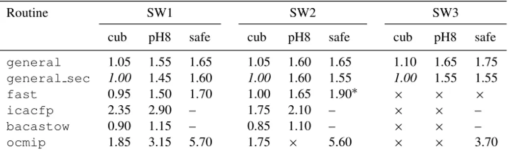
The module mod phsolvers provides six different solvers:
1. the functionsolve at general: the new algorithm described above;
2. the function solve at icacfp: a fixed-point only ICAC method;
3. the function solve at bacastow: Bacastow’s method, an ICAC method with secant iterations (with secant iterations either on [H+] or on its scaled inverse);
4. the function solve at general sec: the variant of solve at general that uses secant instead of Newton–Raphson iterations;
5. the function solve at ocmip: a re-implementation of the OCMIP solver with Newton–Raphson/bisection iterations, completed with a bare minimum of error trap-ping and fitted with the optional initialization scheme common to all of the solvers (the latter was only adapted to use an interval of±0.5 pH unit interval around an op-tional initial value to emulate the recommended OCMIP set-up after start-up);
6. the functionsolve at fast: a simplified version of solve at general without the bracketing control (may not always converge).