Bol. Ciênc. Geod. vol.21 número2

(1)

Bol. Ciênc. Geod., sec. Artigos, Curitiba, v. 21, no_{2, p.329-339, abr-jun, 2015.}

Artigo

LEAST SQUARES FITTING OF ELLIPSOID USING ORTHOGONAL

DISTANCES

Adequação do elipsóide usando distâncias ortogonais com mínimos quadrados

SEBAHATTIN BEKTAS

OndokuzMayis University, Faculty of Engineering, Geomatics Engineering, 55139 Samsun,

sbektas@omu.edu.tr

Abstract:

In this paper, we present techniques for ellipsoid fitting which are based on minimizing the sum of the squares of the geometric distances between the data and the ellipsoid. The literature often uses “orthogonal fitting” in place of “geometric fitting” or “best-fit”. For many different purposes, the best-ﬁt ellipsoid fitting to a set of points is required. The problem of fitting ellipsoid is encountered frequently in theimage processing, face recognition, computer games, geodesy etc. Today, increasing GPS and satellite measurements precision will allow usto determine amore realistic Earth ellipsoid. Several studies have shown that the Earth, other planets, natural satellites, asteroids and comets can be modeled as triaxial ellipsoids Burša and Šima (1980), Iz et al (2011). Determining the reference ellipsoid for the Earth is an important ellipsoid fitting application, because all geodetic calculations are performed on the reference ellipsoid. Algebraic fitting methods solve the linear least squares (LS) problem, and are relatively straightforward and fast. Fitting orthogonal ellipsoid is a difficult issue. Usually, it is impossible to reach a solution with classic LS algorithms. Because they are often faced with the problem of convergence. Therefore, it is necessary to use special algorithms e.g. nonlinear least square algorithms. We propose to use geometric fitting as opposed to algebraic

ﬁtting. This is computationally more intensive, but it provides scope for placing visually

apparent constraints on ellipsoid parameter estimation and is free from curvature bias Ray and Srivastava (2008).

Keywords: Fitting Ellipsoid; Orthogonal Fitting; Algebraic Fitting; Nonlinear Least Square Problem.

Resumo: Neste trabalho, apresentamos a adequação do elipsóide com base na soma dos mínimos quadrados das distâncias geométricas entre os dados e o elipsóide. A literatura

muitas vezes aborda a “adequação ortogonal” em lugar da “adequação geométrica” na “melhor adequação”. Para muitos propósitos diferentes, a melhor adequação do elipsóide para

(2)

elipsóide adequado para a Terra é importante porque se aplica a todos os cálculos geodésicos que são executados sobre o elipsóide de referência. Métodos adequados algebricamente resolvem o problema de adequação por mínimos quadrados lineares, e são relativamente rápaidos e diretos. A adequação do elipsóide ortogonal é um assunto difícil. Normalmente, é impossível encontrar uma solução com algorítimos clássicos de mínimos quadrados. A razão é que eles são frequentemente encontrados com problemas de convergência. Portanto, é necessário usar algorítimos especiais, por exemplo, algorítimos de mínimos quadrados com não lineares. Nós propomos o uso da adequação geométrica em contraste com a adequação algébrica. Isto é computacionalmente mais intensivo, mas dá margem ao uso de injunções relativas na estimação a dos parâmetros do elipsóide e elimina as tendências da curvatura, Ray e Srivastava (2008).

Palavras-chave: Adequação do Elipsóide; Adaptação Ortogonal; Adequação Algébrica; Problema de Mínimos Quadrados Não-Linear.

1. INTRODUCTION

Fitting an ellipsoid to an arbitrary set of points is a problem of fundamental importance in many wide fields of applied science ranging from astronomy, geodesy, digital image processing and robotics to metrology etc. Ellipsoids, though a bit simple in representing 3D shapes in general, are the only bounded and centric quadrics that can provide information of center and orientation of an object. Fitting ellipsoid has been discussed widely and some excellent work has been done in literature. However, most of these fitting techniques are

algebraic fitting, but not orthogonal fitting. Various “least- squares” fitting approaches have been formulated over the years Zhang (1997), but they all fall into two categories; (1) algebraic methods, which are extensively used due to their linear nature, simplicity and computationally efficiency, and (2) geometric methods that solve a nonlinear problemRay and Srivastava (2008).

We could not find enough studies with numerical examples in the literature. Turner et al (1999) gave a numerical application, but the application’s data are not given Turner et al (1999). No other comparable orthogonal fitting ellipsoid application could be found in literature. Against this background, the purpose of the study is to give an orthogonal fitting ellipsoid with numerical examples. In this article, we demonstrate that the geometric fitting approach, provides a more robust alternative than algebraic fitting approach-although it is computationally more intensive.

The paper has eight parts. First, the basic ellipsoid will introduce some mathematical equationsto explainthe concepts. Then, it reviews the extended literature relevant to ellipsoid fitting. And we discussed in this research which estimators is used. Next, comes the part which deals with algebraic fitting, orthogonal fitting and numerical example. You will find ellipsoid fitting application based on both l1-norm and l2-norm methods. The paper concludes

with a discussion of theoretical and managerial implications and directions for further research.

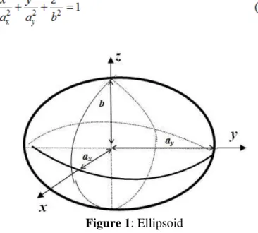
1.1 Ellipsoid

(3)

“ellipsoid” in place of “biaxial ellipsoid, rotational ellipsoid or ellipsoid revolution”. Older literature uses ‘spheroid’ in place of rotational ellipsoid. The standard equation of an ellipsoid

centered at the origin of a cartesian coordinate system and aligned with the axes is shown with this formula:

Figure 1: Ellipsoid

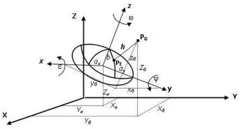
Although ellipsoid equation is quite simple and smooth, computations are quite difficult on the ellipsoid. The main reason for this difficulty is the lack of symmetry. Generally, an ellipsoid is defined with 9 parameters. These parameters are; 3 coordinates of center (Xo,Yo,Zo), 3 semi-axes (ax, ay, b) and 3 rotational angles (, , ) which represent rotations

around x-,y- and z- axes respectively in Figure 2. These angles control the orientation of the ellipsoid.

R1,R2,R3 are plane rotation matrices

(4)

Figure 2: Shifted - oriented ellipsoid

2. FITTING ELLIPSOID

For the solution of the fitting problem, the linear or linearized relationship, written between the given data points and unknown parameters (one equation per data points), consists of equations, including unknown parameters.

Here, A is design matrix, x is unknown parameters, lis measurements vector or data points, For this minimization problem to have a unique solution the necessary conditions is to be n>= 9 and the data points lie in general position (e.g., not all data points should lie is an elliptic plane). Throughout this paper, we assume that these conditions are satisfied.

u=9 : number of unknown parameter

n: number of given data point (or measurements)

f=n-u :degree of freedom

-If f = 0 there is only one (exact) solution, algebraic solution

-If f<0 there is no solution. The solutioncan be found with based on the extra constraint -If f> 0 is most commonly encountered situation. The given data points (or measurements), which are much greater than the required number cause discrepancy, and in this case, the solution is not unique. There is an over determined system. Because n > u, in other words the number of equations is greater than the number of unknowns.

The system of linear equations (3) must be solved. Therefore, this system must be consistent with the rang of design matrix, and design matrix extended with constant terms, must be equal, so that rang(A) =rang(A:l); whereas, the system of (3) is inconsistent, because x

(5)

Depending on the choice of  residuals vector, infinite solutions can be obtained. The unique solution can be derived only according to an estimator (objective function). For example, the LS always give an unique solution Bektas and Sisman (2010). Here, the question of which estimation method to use comes to mind?

3. WHICH ESTIMATOR SHOULD BE USED?

It is hoped that the residuals will be small. The more suitable estimation method is one that creates smaller residuals. It is seen that usually the objective functions are formed based on the minimization of corrections or a function of corrections. There are numerous estimators, some of these are l1-norm, l2-norm,lp-norm, Fair, Huber, Cauchy, German-McClure, Welsch and Tukey. Two estimator methods come to the forefront.The most used estimators are shown below:

(i) [] = min. ( l2-norm) Least Squares Method (LSM)

(ii) [II] = min. ( l1-norm) Least Absolute Values Method (LAVM).

3.1. The Comparison of l1

and l2

-Norm Methods

The solution of the l2-norm method is always unique, and this solution is easily calculated. The l2-norm method is widely used in parameters estimation. The l2-norm method has indisputable superiority in parameter estimation.

The disadvantages of the l2-norm method are that is affected by outlying (gross errors) and it distributes to the sensitivity measurements. In this case, ellipsoid fitting is a very nice application.

With least-squares techniques, even one or two outliers in a large set can wreak havoc! Outlying data give an effect so strong in the minimization that the parameters thus estimated by those outlying data are distorted. Numerous studies have been conducted, which clearly show that least-squares estimators are vulnerable to the violation of these assumptions. Sometimes, even when the data contains only one bad measurement, l2-norm method estimates may be completely perturbed Zhang (1997).

The solution of the l1-norm method is not always unique, and there may be several solutions. Also, the solution of the l1-norm method is not generally obtained directly, but iteratively calculations are made. Therefore, the solution is not easily calculated like in the l2-norm method. Notwithstanding, when the computational tools, computer capacity and speed are considered, the difficulty of calculations are eliminated. The advantages of the l1-norm method are non-sensitivity against measurements, including gross errors, and the solution is not or is little affected by these measurements.

The author of this study proposed and used the l2-norm method in the solution of parameter estimation (optimization problems, adjustment calculus), after the measurement group cleaned up gross and systematic errors using the l1-norm method. For further information see Bektas and Sisman (2010).

(6)

The general equation of an ellipsoid is given as

(5) contains ten parameters. In fact, nine of those ten parameters are independent. For example, if all the coefficients in this equation multiply by (-1/K’), we get a new equation

which contains nine unknown parameters, and its constant term will be equal to “-1”.

In this algorithm, we need to check whether a fitted shape is an ellipsoid. In theory, the conditions that ensure a quadratic surface to be an ellipsoid have been well investigated and explicitly stated in analytic geometry textbooks. An ellipsoid can be degenerated into other kinds of elliptic quadrics, such as an elliptic paraboloid. Therefore, a proper constraint must be added. Li and Griffiths gave the following definitions Li and Griffiths (2004).

However 4j-i2> 0 is just a sufficient condition to guarantee that an equation of second degree in three variables represent an ellipsoid, but it is not necessary. In this paper, we assume that these conditions are satisfied.

The algebraic method is a linear problem. It is solving the problem directly and easily. The fitting ellipsoid to a given the data set ((x,y,z)i , i=1,2,…,n), is obtained by the solution in the LS sense of in the following:

Where

nxu = Design matrix

vu = [ A B C D E F G H I ]Tunknown conic parameters

ln= [1 1 1…1]T unit vector : right side vector

ith row of the nx9 matrix 

It is solved easily in the LS sense as below

or it is solved easily by MATLAB as below

If there are differences in weights or correlations between given data points, P weight matrix is added in the solution, and then

(7)

LS optimization give us |||| =min.

Algebraic methods all have indisputable advantages of solving linear LS problems. The methods for this are well known and fast. However, it is intuitively unclear what it is we are

minimizing geometrically in (6) is often referred to as the “algebraic distance” to be

minimized Ray and Srivastava (2008). A geometric interpretation given by Bookstein (1979) clearly demonstrates that algebraic methods neglect points far from the center.

5. FITTING OF ELLIPSOID USING ORTHOGONAL

DISTANCES

To overcome the problems with the algebraic distances, it is natural to replace them by the orthogonal distances which are invariant to transformations in Euclidean space and which do not exhibit the high curvature bias. An ellipsoid of best fit in the LS sense to the given data points can be found by minimizing the sum of the squares of the geometric distances from the data to the ellipsoid. The geometric distance is defined to be the distance between a data point and its closest point on the ellipsoid.

Determining best fit ellipsoid is a nonlinear least squares problem which in principle can be solved by using the Levenberg-Marquardt (LM)algorithm. Generally, non-linear least squares is a complicated issue. It is very difficult to develop methods which can find the global minimizer with certainty in this situation. When a local minimizer has been discovered, we do not know whether it is a global minimizer or one of the local minimizer Zisserman (2013). There are a variety of nonlinear optimization techniques. Such as Newton, Gauss-Newton, Gradient Descent, Levenberg-Marquardt approximation etc.However, these fitting techniques involve a highly nonlinear optimization procedure, which often stops at a local minimum and cannot guarantee an optimal solution Li and Griffiths (2004).

Away from the minimum, in regions of negative curvature, the Gauss-Newton approximation is not very good. In such regions, a simple steepest-descent step is probably the best plan. The Levenberg-Marquardt method is a mechanism for varying between steepest-descent and Gauss-Newton steps depending on how good the HGN approximation is locally.

The Levenberg-Marquardt method uses the modiﬁed Hessian H(x,λ) = HGN +λ.I ( I : identity matrix )

• When λ is small, H approximates the Gauss-Newton Hessian.

• When λ is large, H is close to the identity, causing steepest-descent steps to be taken.

This algorithm does not require explicit line searches. More iterations than Gauss-Newton, but, no line search required, and more frequently converge suppose that we have a unknowns parameter set

v= [ A B C D E F G H I ]T are unknown conic parameters. The general conic equation for an ellipsoid is given as (6)

We will reach the solution by establishing relationships between variations in the conical coefficients and the orthogonal distances.

The initial parameters were derived from the algebraic fitting ellipsoid.

(8)

ith row of the nx10 matrix J (jakobien matrix)

ith row of the right side vector hnx1

We obtained the below linearized equation

The fitted orthogonal ellipsoid is obtained by the solution in the LS sense with the L-M algorithm.

5.1 The Levenberg-Marquardt

Algorithm

1-Solve algebraic methods and find initial values for v

set λ=1 (say)

2- Compute J-jacobien matrix and hi orthogonal distances from all given data points

minh= hT_h

3- Solve ( JTJ + λ I ) dv= JT_h

v=v+dv , new conic parameter

Find again hi orthogonal distances from all given data points

newh= hTh

4- ifnewh<minh % yes there is improvement, reduce λ

minh=newh; λ=λ/2

goto 3

else % no improvement, increase λ

λ=2*λ

goto 3

end

(9)

In this paper, we present techniques for ellipsoid fitting which are based on minimizing the sum of the squares of the geometric distances between the data and the ellipsoid. The most time-consuming part is the computation of the orthogonal distances between each point and the ellipsoid. Our aim to find the orthogonal distances from a shifted-oriented ellipsoid see Figure 2. For detailed information on this subject refer to Bektas (2014).

6. NUMERICAL EXAMPLE

For numerical applications 12 triplets (x,y,z) cartesian coordinates were produced. Here data points coordinates,

x: [ 7 7 9 9 11 11 8 8 10 10 12 12 ] y: [22 19 23 19 24 20 21 17 22 18 23 19 ] z: [31 28 31 27 29 26 32 29 32 28 31 28 ]

This problem is also solved by Least Absolute Values Method( l1-norm) and the following results were obtained.

The conical coefficients in the Least Squares Method is,

v=[-0.0006 -0.0008 -0.0010 0.0005 -0.0005 0.0003 0.0092 0.0050 0.0278] The conical coefficients in the Least Absolute Values Method is,

v=[ -0.0071 -0.0084 -0.0096 0.0047 -0.0040 0.0023 0.0880 0.0061 0.0271]

We show both the algebraic and orthogonal fitting results are as shown in Table-1.

Table-1: The result of algebraic and orthogonal fitting ellipsoid

*RSS: The residual sum of squares of the orthogonal distances

7. DISCUSSION

Orthogonal least-squares has a much sounder basis, but is usually difficult to implement. Why are algebraic distances usually not satisfactory? The big advantage of use of algebraic distances is the gain in computational efficiency, because closed-form solutions can usually be obtained. In general, however, the results are not satisfactory.The function to minimize is usually not invariant under Euclidean transformations. For example, the function with

(10)

of noise, it is desirable for them to contribute the same way Zhang (1997). More importantly, algebraic methods have an inherent curvature bias – data corrupted by the same amount of

noise will misﬁt unequally at different curvatures Ray and Srivastava (2008). Our experience tells us that if the coordinates of given points consists of a large number this will cause bad condition. Therefore, before fitting, you must shift the given coordinates to the center of

gravity, after fitting operation the coordinates of ellipsoid’s center must be shifted back to the previous position.

8. CONCLUSION

In this paper, we studied on the orthogonal fitting ellipsoid. The problem offitting ellipsoid is encounteredfrequently intheimage processing, face recognition, computer games, geodesy-determiningmore realistic Earth ellipsoid etc. The paper has presented a new method of orthogonal fitting ellipsoid. The new method relies on solving an over determined system of nonlinear equations with the use of the L-M method. In conclusion, the presented method may be considered as fast, accurate and reliable and may be successfully used in other areas. The presented orthogonal fitting algorithm can be applied easily to biaxial ellipsoid, sphere and also other surfaces such as paraboloid, hyperboloid,etc.

REFERENCES

Bektas, S., Sisman, Y. The comparison of L1 and L2-norm minimization methods,

International Journal of the Physical Sciences, 5(11), 1721 – 1727, 2010

Bektas, S. “Orthogonal Distance From An Ellipsoid, Boletim de CienciasGeodesicas, Vol. 20, No. 4 ISSN 1982-2170 , http://dx.doi.org/10.1590/S1982-217020140004000400053 (in Press), 2014

Bookstein, F. L. Fitting conic sections to scattered data”, Computer Graphics and Image Processing 9,56-71, 1979.

Burša M, Šima Z. Tri-axiality of the Earth, the Moon and Mars, Stud. Geoph.etGeod. 24(3):211–217, 1980.

Eberly, D. Least Squares Fitting of Data”, Geometric Tools, LLC, http://www.geometrictools.com, 2008.

Feltens, J. Vector method to compute the Cartesian (X, Y ,Z) to geodetic (, λ, h) transformation on a triaxial ellipsoid”, Journal of Geod. 83:129–137, 2009.

İz, H. B., Ding X. L., Dai C. L.,Shum C. K. Polyaxial figures of the Moon, J. Geod. Sci., 1, 348-354, 2011.

Li, Q., Griffiths J.G. Least Squares Ellipsoid Specific Fitting, Proceedings of the Geometric Modelling and Processing (GMP’04), 2004.

(11)

Ray, A., Srivastava D.C. Non-linear least squares ellipse fitting using the genetic algorithm with applications to strain analysis, Journal of Structural Geology 30 1593-1602. 2008.

Turner, D.A., Anderson I. J., Mason J.C., Cox, M.G. An algorithm for fitting an ellipsoid to data, Cite-dataseerXBeta, http://citeseerx.ist.psu.edu/viewdoc/summary? doi=10.1.1.36.2773, 1999.

Zhang, Z. Parameter estimation techniques: a tutorial with application to conic fitting, Image and Vision Computing 15,59-76, 1997.

Zisserman, A. C25 Optimization, 8 Lectures, Hilary Term 2013,2 Tutorial Sheets,Lectures 3-6 (BK), 2013.